

Abstract
Range-resolved interferometry (RRI) allows the simultaneous demodulation of multiple interferometric signal sources and provides a tomographic view of all constituent interferometers that may be present in a setup. Through comparison with a reference distance of known length, absolute distance measurements can be performed. RRI is tailored to the use of laser frequency modulation through injection-current modulation of regular, monolithic laser diodes that are both cost-effective and highly coherent and therefore this approach promises broad applicability. In this paper, two methods for absolute distance measurement, one based on the direct evaluation of the signal peak positions and one based on the phase demodulation of an additional lock-in modulation signal, are experimentally demonstrated. Using an external verification displacement interferometer, both techniques are shown to achieve in-situ absolute distance measurements with systematic errors below  over a 50 mm travel range. The aim of this paper is to establish the general suitability of RRI for absolute distance measurements and in-situ tomographic interferometer characterisation for precision engineering. In future, this approach could be used to diagnose interferometric setups for parasitic signal contributions, multiple reflections or to determine the dead path length for accurate environmental compensation, either for use during initial setup of, or for continuous operation alongside, a regular displacement measuring interferometer.
Export citation and abstract BibTeX RIS

Original content from this work may be used under the terms of the Creative Commons Attribution 4.0 license. Any further distribution of this work must maintain attribution to the author(s) and the title of the work, journal citation and DOI.
1. Introduction
High-performance interferometric displacement measurements are a key enabling technique for many areas of nanotechnology and precision engineering [1–5]. This is because interferometers offer remote displacement measurements at sub-nanometre resolution that are, through knowledge of the laser vacuum wavelength and the index of refraction (for measurements in air), a fundamental representation of the metre definition [6–8]. Usually the fractional frequency stability of stabilised Helium-Neon laser is on the order of 10−9 [7] and stabilities as low as 10−12 can be reached with advanced approaches such as frequency combs [9]. Therefore in many cases laser frequency stability is not a dominant source of uncertainty, however, interferometers do often suffer from uncertainties due to periodic non-linearities [10–13], also termed cyclic errors,, i.e. errors that are periodic at integer fractions of the laser wavelength. Periodic non-linearities mainly originate from polarisation leakage or from parasitic or multiple reflections. Periodic non-linearities typically lead to uncertainties in the nanometre to sub-nanometre ranges but, using sophisticated correction methods, these can sometimes be reduced to values of several tens of picometres or below [14–18]. However, even if advanced correction methods are available for many situations, reducing them in the first place through their range-dependent identification using a tomographic view of the interferometric setup would provide better knowledge on their origin and thus give a better ability to suppress them. This is especially true for periodic non-linearities caused by multiple reflections [13, 19] that are very alignment sensitive. Therefore, such a tomographic view would be highly desirable as a diagnostic tool and could be a route to routinely lower uncertainties originating from periodic non-linearities in interferometric practice.
Furthermore, in many situations uncertainties due to the lack on knowledge of the air refractive index remain the dominant uncertainty source for interferometric measurements in air. The air refractive index, due to its dependence [20] on air temperature, air pressure and humidity, amongst others, can typically vary in the range of several parts-per-million (ppm), which would lead to correspondingly high uncertainties in the displacement measurement. In order to counteract air refractive index uncertainties, the environmental air parameters are usually measured using external sensors in an environmental compensation unit and interferometric measurements are then compensated using the Edlén formula [21] or its refinements [22, 23]. Even assuming an otherwise ideal refractive index compensation, it is an often overlooked fact that any error in the knowledge of the dead path length [24], i.e. the optical path difference (OPD) at the position where the interferometer was initialised, can lead to significant non-recoverable errors in the air refractive index compensation during the measurement. For interferometers at the highest accuracy levels, given that significant changes of the air refractive index can easily occur during the course of a measurement campaign, the direct determination of the dead path to accuracy levels well below millimetres is therefore very important.
In this paper, an interferometric technique, based on cost-effective diode lasers, that could supplement regular high-precision interferometers with diagnostic data is proposed. In particular, both for the provision of a tomographic view to identify to contribution of undesired signal sources as well as for the direct measurement of the dead path, a measurement technique that provides in-situ absolute distance measurements of multiple signal sources present within an interferometer assembly would be highly desirable. Additionally, a tomographic view capability, even at a relatively coarse resolution (μm to mm) could be very useful from a practical perspective. During setup it would allow better control of the alignment by providing direct user feedback on the signal strength at a given range. Also, if used on a positioning unit, it would allow an initial estimate of the stage position, for example to prevent damage during referencing runs. Furthermore, such a system could serve as a warning system that would be able to detect if cumulated tracking errors have exceeded a certain level. This would be especially beneficial in situations where signal loss due to low light levels, beam interruption or very high travel velocities cannot be ruled out.
Of course, absolute measurement capabilities that could be used for in-situ absolute distance measurements of multiple signal sources in interferometric setups are possible to achieve in a number of ways. These include frequency scanning interferometry [25–28] using widely modulated highly coherent external cavity lasers or the use of optical frequency combs, either used directly as pulsed lidar [29] or employed to calibrate the modulation waveform in frequency-modulated continuous-wave (FMCW) lidar [30]. These methods achieve very high, sub-micrometre accuracies and can resolve multiple signal sources to provide a tomographic view, however, they typically require a very complex and expensive setup. Furthermore, frequency scanning interferometry is very vibration sensitive [28], due to the low laser scanning speeds of the mechanically tuned external cavity lasers typically used, causing further uncertainties, particularly for measurements outside precision metrology environments. For dead path characterisation, in some cases it is possible to initialise the interferometer at the balance point, i.e. the position in the measurement arm where the OPD is zero and where consequently the dead path is also zero. For example, the balance point can be determined through modulation of the laser frequency and finding the position where the interferometric phase variation is minimised [14]. Also, low-coherence interferometry [31] can be used to define the zero-position of the interferometer with sub-micrometre resolution. However, for many interferometer designs, for practical reasons the balance point cannot be part of the travel range of the measurement arm, or some interferometer designs cannot be balanced for principle reasons, for example Fabry–Perot configurations, and in these cases an independent in-situ measurement of the dead path length would be highly desirable. Also, some commercial interferometer systems [32] based on laser diode wavelength modulation offer additional absolute distance measurements, but typically only with a resolution on the order of 1% of the working distance and also only under the assumption of a single, dominant signal source without providing the capability to demodulate multiple interferometric sources and to provide a tomographic view of the setup.
In this paper, the use of range-resolved interferometry (RRI) [33] for absolute distance measurements of multiple signal sources at error levels below  is proposed. RRI is tailored to use of laser frequency modulation through injection current modulation of single-mode monolithic laser diodes that are both robust and highly coherent. Also, RRI can be implemented on cost-effective off-the-shelf signal processing hardware, therefore, a very cost-effective system based on this approach is feasible at least for some laser wavelengths. This could make it possible to integrate such a system into measurement systems where previously integration was prohibitive due to the high cost and system complexity involved. The proposed approach could also be readily retrofitted into existing fibre-coupled or free-space interferometric setups, and used either for initial diagnostics of the interferometer assembly, temporarily replacing the measurement laser, or, alongside the main measurement laser to enable continuous monitoring of the interferometer during operation. This paper aims to perform the first qualification of absolute distance measurements based on RRI for high-accuracy applications. Previously, absolute distance measurements using RRI have only been used for in-process coherent laser ranging for manufacturing applications [34], however, here the accuracy has not been evaluated to satisfy the needs of precision engineering and metrology. In this paper, two evaluation methods using RRI measurements are analysed, where in both methods measurements from a target with unknown distance are compared to a fixed reference at a known length defined by a gauge block. In the first method, the range is directly derived from the position of the range-dependent signal peaks in the RRI tomographic view, while in the second method, first proposed in this paper, an additional sinusoidal laser wavelength modulation is applied and its range-dependent phase excursion amplitude determined using a lock-in approach. In the experimental sections, both methods for distance measurements are compared in a variety of settings, including dynamic, stationary and stability measurements, and the accuracy is also verified using an additional commercial displacement measuring interferometer. Finally, a detailed discussion of the merits and options for improvements of the two proposed methods is presented and ideas for their potential use are explored.
2. Methods
2.1. Absolute distance measurements through direct peak evaluation
The first method to be used for absolute distance measurement is the direct evaluation of the range-dependent demodulation phase carrier amplitude  [33] in RRI. This is analogous to the tomographic view as a function of the OPD provided by a Fourier transform of the interferogram in swept-source frequency domain optical coherence tomography [35], frequency scanning interferometry [25], optical frequency domain reflectometry [36] or FMCW lidar [37]. These techniques use linear (sawtooth ramp or triangular) laser frequency modulation waveforms and, in ideal conditions, a simple Fourier transform of the resultant interferogram provides a tomographic view of the signal amplitude as a function of OPD of the constituent interferometers present. In contrast, RRI uses low-complexity sinusoidal laser frequency modulation waveforms where only a sinusoid constituting a single frequency component in applied, but where consequently a more complex demodulation approach using a series of unique, range-dependent carrier signals is required to obtain the tomographic information. In general, the complexity with linear techniques arises due to the practical difficulty of obtaining linear waveform sweeps because of the many harmonics involved in the modulation waveform [38, 39]. Therefore linear techniques require either complex laser designs that can natively perform linear sweep waveforms, the use of a sweep-reference interferometer with associated signal processing chain to re-sample the data acquisition to match the actual sweep conditions or the adaptive pre-shaping of the sweep waveform [39]. RRI on the other hand, due to its simple and consequently very stable modulation regime can work in a very basic setup without sweep-reference interferometer, using only a monolithic laser diode, thereby moving complexity from the optical to the electronic signal processing domain, where it is likely to lead to more cost-effective and robust solutions.
In the setup for the present paper, the contributions of two signal sources at different ranges, the reference and the target interferometers, are simultaneously present in the interferogram. By comparing the ratio of two range values, and with the reference range at a known length, the absolute target distance can be determined. The principle of the method is illustrated in figure 1. Here, the interferogram is evaluated and the demodulated signal amplitude plotted against the demodulation phase carrier amplitude  [33], i.e. the phase excursion of the carrier that is used to demodulated the interferogram resulting from sinusoidal laser frequency modulation in RRI. Using the assumption that the measured distances are short compared to the distance corresponding to the time-of-flight of the sinusoidal modulation waveform of period
  , the
, the  value of the peak position should be directly proportional to the OPD of an interferometer present in the setup [33] and an example tomographic view is shown in figure 1(a). The determination of the peak positions then allows the OPDs of each signal source present to be determined.

Figure 1. Illustration of direct peak position determination method. Here, (a) shows a tomographic view of the range dependency of a signal with both reference and target interferometers present, (b) then plots the natural logarithm of plot (a) and (c) shows the peak position determination through differentiation of plot (b) and location of the zero-crossing through interpolation of the straight line resulting from differentiation.
Download figure:
Standard image High-resolution imageIn the proposed technique, in order to make it compatible with real-time measurements, the signal amplitude is evaluated at a limited number of regularly spaced evaluation locations along the  axis, termed range channels. Depending on the chosen Gaussian window width parameter used in the RRI demodulation [33], where a Gaussian window width parameter of σ = 0.05 is used in this work, a distance between range channels of
  is chosen. However, it is stressed that this is only an initial choice and a detailed investigation on the optimal parameter choices is still outstanding. In this way, range channels are close enough that several evaluation locations (at least 3) cover the peak in every possible position, as illustrated in figure 1(a). Because the shape of the peak is defined by the Gaussian window function used in the RRI signal processing it will also be a Gaussian shaped exponential function of the form
  in the
  plot. Consequently, the natural logarithm of the range signal will correspond to a parabola, as shown in figure 1(b). When the local slope of the parabolic signal at the evaluation locations is calculated through differentiation, a straight line will then result as shown in figure 1(c). The zero-crossing of this line equals the desired peak position, and is found through linear interpolation from the two range channels just before and just after the sign change. Please note that in order to preserve symmetry, the value of the differentiation of a pair of range channels is assigned to the middle of the range in between them, as also illustrated in figure 1(c).
2.2. Absolute distance measurements though lock-in phase modulation
A further method for absolute distance measurements is the use of an additional, slow laser frequency modulation waveform, leading to a range-proportional phase signal after phase demodulation for each constituent interferometer. The amplitudes of these phase signals can then be recovered using lock-in techniques. To implement this method, the injection current of the laser diode is modulated simultaneously with two sinusoids, one fast, high-amplitude sinusoid with modulation period  , identical to the one used in the first method in section 2.1, and one additional slow, low-amplitude sinusoid of period
  . Here, the fast modulation signal is used to perform interferometric signal processing and phase determination using the RRI technique in the usual way [33], while the slow modulation then yields a measurable phase signal whose amplitude can be determined. As in all laser wavelength modulated interferometers, the amplitude of the phase excursion is directly proportional to the OPD of the constituent interferometer.
In the proposed method, the phase of the interferometer is demodulated at a single range channel each for both reference and target interferometers, approximately located on the top of the respective peaks as illustrated in figure 2(a). The resulting phase signals over one modulation period  of the slow laser frequency modulation waveform are shown in figure 2(b). The phase excursion amplitude recorded for each constituent interferometer should then be directly proportional to its OPD and the amplitude of the sinusoids can be easily recovered through lock-in demodulation as the applied modulation is synchronous to the data acquisition. Again, by calculating the ratio between the phase excursion amplitude of the target and the reference interferometers, the target distance can be determined.
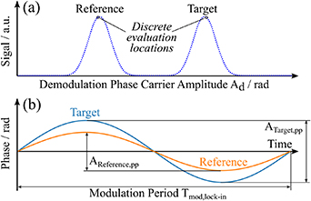
Figure 2. Illustration of the lock-in phase modulation method. (a) shows the evaluation locations of the phase signals of the reference and target interferometers using a single range channel for each peak. (b) Then plots a time plot of the phase signals resulting from the additional slow phase modulation over one modulation period  , with the range-dependent peak-to-peak amplitude for the target and reference signals indicated.
Download figure:
Standard image High-resolution image3. Experimental setup
The experimental setup to test the proposed methods is shown in figure 3. Here, the demonstration setup is shown in the upper half of figure 3, while the lower half shows the interrogation unit and both parts are connected using regular single-mode optical fibre. The demonstration setup consists of two low-finesse Fabry–Perot interferometers, one stationary interferometer, serving as a length reference, and the moving target interferometer. An annotated photograph of the interferometer assembly is also shown in figure 4. Both reference and target interferometers are designed so that they each contain exactly two reflections sources that form the respective interferometer. The fibre lead length from the fibre coupler to both interferometers differs by ≈1 in order to avoid undesired mutual interferences between reflections in the reference and target interferometers. Any interferences occurring across the two coupler arms, due to their larges OPDs ≈1
 , now have fringe rates that are well outside the bandwidth of the low-pass filter placed before the analogue-to-digital converter (ADC), as shown in figure 3, and therefore any additional signal contributions caused by these interferences is strongly suppressed.

Figure 3. The fibre-coupled experimental setup is illustrated, where the upper half shows the target and reference interferometers along with the external verification interferometer. The lower half then illustrates the interrogation system using a laser diode and an off-the-shelf signal processing board.
Download figure:
Standard image High-resolution image
Figure 4. Annotated photograph of the interferometer assembly, including the reference interferometer placed in the front, the stage-mounted target interferometer and the commercial verification interferometer on the right.
Download figure:
Standard image High-resolution imageThe reference interferometer consists of a gradient index lens butt-coupled onto a rectangular glass flat block with index-matching gel to result in only one reflection point at the internal air-to-glass interface of the block. The distal reflection is provided by the front surface of a glass block and a diffusing coating is applied on the back surface of the glass block in order to prevent back-reflections. The two glass blocks are spaced by a gauge block (class 1 according to DIN EN ISO 3650) of 50.000 mm length and the glass blocks are attached to the gauge block using contact bonding. It is estimated that the accuracy of the reference length is below 1 μm, including all contributions from the gauge block tolerance, temperature variations, bonding procedure and glass block flatness.
The target interferometer uses the Fresnel reflection from the tip of the fibre lead as a first reflection point and the reflection from a wedge mirror target as the second reflection point placed on the moving linear step-motor stage with a maximum travel range of 50 mm. An anti-reflection coated lens assembly is used to collimate the beam emanating from the fibre. Furthermore, a commercial interferometer using a Helium-Neon laser (SIOS MI 5000) is pointing at an additional retroreflector, placed on the back of the moving stage, allowing it to verify the actual stage displacement with high accuracy. For the comparison between the target and the verification interferometer, the dominant error source is deemed to be the cosine errors due to imperfect alignment of the two interferometer beams. Reasonable care has been taken to avoid cosine errors by minimising beam wander over the travel range. Also, Abbe errors [40] cannot be ruled out due to the non-zero offset between the measurement and reference axis, however, Abbe errors are expected to stay at or below 1 μm. Nevertheless, for the accuracy levels targeted in this work (μm to mm), both cosine and Abbe errors are considered small and subsequently neglected.
The optical fibre-coupled interrogation unit is shown in the lower parts of figure 3. For signal modulation and acquisition a commercial off-the-shelf low-cost Nucleo-H743ZI2 board by STMicroelectronics, based on the STM32H7 family controller, is used. The two on-board digital-to-analogue convertera (DAC) can generate two synchronous, sinusoidal waveforms. The fast waveform of frequency  is used to provide laser wavelength modulation for the RRI signal processing. An optional slow sinusoidal waveform of modulation frequency
  can be added to the fast modulation waveform to implement the additional lock-in technique described in section 2.2. The resulting modulation waveform is then used to modulate the injection current of an Eblana EP1550-0-DM-B01-FA discrete mode laser diode (Wavelength:
  ; Linewidth:
  ) via the modulation input of a laser driver unit. The peak-to-peak current modulation amplitudes are
  for the fast and
  for the slow modulation waveform, corresponding to a peak-to-peak optical wavelength modulation amplitudes of 308 and
  , respectively.
The emitted fibre-coupled laser light passes through a fibre-optic circulator, is evenly split by a directional coupler and then travels to the two interferometers. On return, light from both interferometers is guided by the circulator to a photo detector. The resulting signal is sampled using the on-board 16 Bit ADC on the Nucleo board at a sample rate of  , where it is of crucial importance to the RRI signal processing that the data acquisition is clock and phase-synchronous to the modulation waveform generation in the DAC channels. The acquired photo detector signal is then transmitted to a PC and a software implemented in the Python programming language executes the RRI signal processing algorithms [33]. In this basic implementation using low-cost hardware, data can be acquired for a maximum of several seconds and is then post-processed over several seconds, however, on previous occasions real-time RRI signal processing has also been demonstrated over extended periods [41, 42], therefore, this is no principle hurdle to the applicability of the technique.
3.1. Range signals
An example photo detector signal corresponding to a single interferogram over one modulation period  is plotted in figure 5(a), along with the Gaussian window function with window width parameter σ = 0.05 used in the RRI signal processing [33] to select the parts of the modulation waveform with the highest fringe frequencies. The resulting range dependency is evaluated from the interferogram as a function of demodulation phase carrier amplitude
  and is shown in figure 5(b). Due to the non-linearity of the laser frequency modulation that occurs in every laser diode even when a perfectly sinusoidal injection current modulation waveform is applied, higher order non-linear corrections of the modulation waveform need to be incorporated into the demodulation carriers. Here, a first carrier harmonic of 4.5% at a phase shift of 5∘, as determined by visual inspection of the symmetry of the demodulation phase carrier amplitude versus signal processing delay maps, was used in the demodulation carriers in addition to the correction of parasitic intensity modulation as previously described [33].

Figure 5. Measured RRI signals. (a) Plots the interferogram as recorded by the photo detector over one modulation period  along with the chosen Gaussian window function used for the RRI signal processing. (b) shows the evaluated range dependency of the signal as a function of
  .
.
Download figure:
Standard image High-resolution imageIn the resulting tomographic view shown in figure 5(b), the reference peak has its maximum at  and the target peak has its maximum located at
  , with full-width half-maximum (FWHM) peak widths of
  . The physical path length of the reference peak is known through the spacing of the gauge block to be
  . Therefore, the scaling factor is
  and the physical path length of the target peak can be determined as
  , with a corresponding peak width (FWHM) of
  . A further peak with low amplitude can be seen at
  , which is likely to be caused by a undesired multiple reflection (double bounce) signal in the reference interferometer. Therefore, figure 5(b) also provides an example of how the tomographic view can be used for in-situ analysis of an interferometer and the detection of multiple reflection signals which are physically present within the interferometer assembly.
In this configuration, in order to ensure that the double bounce signal does not overlap with a target signal, the target signals are restricted to demodulation phase carrier amplitudes well above the double bounce peak. Thus the stage is positioned so that the stage travel range is located between  and
and  , i.e. between 117 and
  . However, as also discussed later, if two separate photo detectors, ADCs and associated fibre components would be used to individually evaluate the target and reference interferometers, no such restrictions would apply and a much wider travel range could be covered.
3.2. Lock-in phase modulation signals
To implement the lock-in technique of section 2.2 the target and reference interferometers are simultaneously demodulated and the amplitude of their respective phase response at the additional modulation frequency  is analysed. Measured phase signals over one lock-in period are shown in figure 6(a) with peak-to-peak phase amplitudes of 22.09 and
  for the reference and target interferometer, respectively. The phase modulation depth of the lock-in signal was chosen to be close to the maximum fringe rate permissible (
 ) at the maximum target range to make use of the highest possible phase signal excursions. Because, as discussed previously, the injection current modulation of a laser diode generally results in a non-linear optical frequency modulation, a first harmonic of the lock-in frequency at non-zero amplitude exists, as visible in figure 6(b), however, due to the lock-in principle this is of no concern to the amplitude measurement of the fundamental sinusoid. Figure 6(c) then plots the residuals of the phase signals after the fundamental sine and the first harmonic are subtracted. The residual signals exhibit standard deviations of 0.04 and
  for the reference and target interferometers, respectively, and this will be, in general, caused by a combination of noise and cyclic errors. However, because no characteristic fringe-speed dependent signal patterns with π or 2π phase distance that would be indicative of strong cyclic errors are discernible and also because very low non-linearities at the mrad levels have previously been demonstrated [33, 43] with RRI, is is likely that the bulk of the residual signals is actually due to noise and not due to cyclic errors. This is important because, unlike noise, cyclic errors could lead to systematic errors in the distance determination for the lock-in technique and therefore they need to be sufficiently low.

Figure 6. An example measured phase signal as a result of the additional laser modulation at  is shown in (a) for the target and reference interferometers. (b) Then shows the signals with the main sine subtracted while (c) plots the residuals with both main sine and first harmonic subtracted.
Download figure:
Standard image High-resolution image4. Results and discussion
4.1. Short ramp measurement
First, in order to investigate the general quality of the measurement data for the two proposed methods, results from an experiment using a  ramp movement are shown in figure 7, recorded over a duration of
  and using the external interferometer to verify the measurements. Here, on the left panels, in figures 7(a) and (b), the results from the direct peak detection method of section 2.1 are shown, while the plots on the right, in figures 7(c) and (d), show results from the lock-in method of section 2.2. Note that these results were recorded at separate instances for the two methods, thus the motion pattern is not exactly identical. In order to allow better comparison of the noise performance of the two methods, the data rate should be identical for both cases. Therefore the results for the direct peak evaluation method are averaged over
  , identical to the native data rate of the lock-in method
  .
.

Figure 7. Short ramp measurements over 10 s with a target ramp movement over  within
  . (a) shows the time series of raw signals and (b) evaluated distance for the direct peak evaluation method, while (c) shows the time series of raw signals and (d) the evaluated distance measurement for the lock-in method. Note that the left and right panels constitute separate experiments.
Download figure:
Standard image High-resolution imageFigure 7(a) shows the raw peak position measurements for the reference and target interferometers, respectively, while figure 7(b) shows the calculated target distance measurement along with the external verification interferometer displacement measurement fitted to the initial, stationary part of the absolute distance measurement. The ramp measurement was repeated using the lock-in method, with results plotted in a similar manner in figures 7(c) and (d). Comparing the distance results for the two methods, it can be seen that the noise levels for the direct peak evaluation method are considerably lower than for the lock-in method. In the static parts of the signals noise standard deviations (1σ) are 18 and 76 μm for figures 7(b) and (d), at  data rate, respectively. A key difference between the two methods lies in the ability to measure during target movements, where the direct peak evaluation method can correctly measure the position during the entire ramp movement, as seen in figure 7(b), while the lock-in method completely fails during the movement of the stage, as seen in figure 7(d). The reason is thought to be due to frequency components in the demodulated phase signal of the ramp movement coinciding with the lock-in frequency and distorting the measurement. In future implementations, this behaviour could be reduced by using higher lock-in frequencies further away from possible target phase signal frequency content, however, in the present setup using the low-cost Nucleo-board, the lock-in method is clearly only suitable for static measurements.
4.2. Long travel measurements
To estimate how linear and accurate both methods perform over a larger distances, the following measurement campaign is performed: the linear stage shifts the target in  steps over a total distance of
  , where at each step 10 measurements are taken, each lasting
  , then the mean value and the standard deviation at each stage position, indicative of the repeatability of the measurement, is calculated. Calculated mean values of the target and reference peak position for the direct peak evaluation method and of the target and reference phase amplitude for the lock-in method are shown in figures 8(a) and (d), respectively. The measured absolute target distance at each stage position coincides well with the relative displacement data measured by the external interferometer as shown in figures 8(b) and (e). Considering the target distance value at the first stage position as an initial null displacement value allows to directly calculate the error of estimated distance measurements with respect to the external interferometer readings.

Figure 8. Step measurement. Direct peak evaluation method: (a) step series, (b) target distance, (c) error of estimated distance with respect to the external interferometer; Lock-in method: (d) step series, (e) target distance, (f) error of estimated distance with respect to the external interferometer. Note that the left and right panels constitute separate experiments.
Download figure:
Standard image High-resolution imageAs plotted in figures 8(c) and (f), noise standard deviations over ten  measurements at a single location vary from 2 to 13 μm for the direct peak evaluation and between 9 and 42 μm for the lock-in method. Therefore the noise standard deviations in the results for the lock-in method exhibit a significantly larger variation at different stage positions in comparison to the direct peak evaluation method, but the direct peak evaluation method also shows some variation. The reason for this wide variation is not immediately clear, but could be explained by different noise levels for different range channels, varying signal strengths or perhaps changes in environmental vibration levels at different stage positions.
Crucially, in figures 8(c) and (f) the mean values of the resulting cumulative distance errors are within  m for both the direct peak evaluation method and for the lock-in method, equating to fractional errors below ±0.1% over the
  travel range. This experiment therefore provides a first estimate of the achievable accuracies for both methods and the accuracy levels demonstrated here are deemed to be sufficient for the purpose of interferometer characterisation and dead path determination in most cases. A separate setup using two adjacent, gauge-block spaced interferometers with transparent windows and illuminated by a single beam [44], were gauge blocks in variable combinations could be inserted, could allow a more formal quantification of the uncertainties involved. This experiment would directly provide an absolute independent reference measurement provided by the additional gauge block, rather than the relative independent reference measurement currently provided by the Helium-Neon interferometer, simplifying the uncertainty analysis, and would also be free from geometrical errors due to the sequential single-beam arrangement, however, such a dedicated setup is beyond the scope of this paper.
4.3. Long-term stability
A long-term measurement is performed to determine the stability and the influence of drift of the laser modulation on the measured distance. This measurement lasted 8 h each for both methods, where the target distance was averaged over  of data with an interval between measurements of 19 s during which the signal is processed, leading to a sample rate of
  . The results are shown in figure 9, again for the direct peak evaluation method on the left panels and for the lock-in method on the right panels, where both experiments were conducted on different nights and are therefore not correlated. For all panels in figure 9, the secondary y-axis is labelled in fractional deviation from the mean in units of parts-per-million (ppm). Here, figures 9(a) and (b) as well as figures 9(d) and (e) show the time series of the reference and target signals, respectively, while the lower panels, figures 9(c) and (f), show the computed distance measurements.
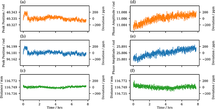
Figure 9. Long-term measurement. Direct peak evaluation method: (a) time series reference, (b) time series target, (c) computed distance measurement; Lock-in method: (d) time series reference, (e) time series target, (f) computed distance measurement. Note that the left and right panels constitute separate measurements recorded at different times and are not correlated to each other.
Download figure:
Standard image High-resolution imageThe obtained results demonstrate that drifts that affect the target signal and the reference signal proportionally, for example a drift in the laser modulation depth, cancel during the distance calculation. For example, for the direct peak evaluation method shown in figure 9 on the left panel, a small jump in the first hour of measurements is clearly visible, with proportionally the same magnitude for the reference peak position and the target peak position shown in figures 9(a) and (b), respectively. However, it can then be seen in figure 9(c) that this does not affect the final calculated distance measurement. As for the lock-in method, there is a clear upward drift for both the target phase amplitude and the reference phase amplitude shown in figures 9(d) and (e), which does not occur in the calculated distance shown in figure 9(f). The computed standard deviations for the  averaged data are 2.7 μm, or
  , for the direct peak evaluation method in figure 9(c) and 5.0 μm, or
  , for the lock-in method in figure 9(f).
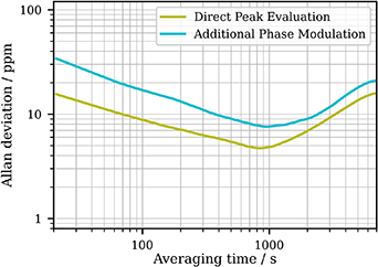
To further investigate the stability behaviour of the techniques, the overlapping Allan deviation [45] of the computed distance measurement data of figures 9(c) and (f) was calculated and is shown in figure 10. Here it can be seen that for averaging times between  until
until  , the Allan deviations drop with a slope of
  per decade, as would be expected for a measurement dominated by white noise. Above
  , the stability decreases again with the onset of drifts, where it is unclear whether these drifts are caused by the measurement device or by environmentally introduced thermal variations in the mechanical setup. However, at the optimum averaging period of
  , Allan deviations below
  were recorded for both techniques, equating to noise standard deviations below 1 μm over a typical measurement distance of
  .
.
Figure 10. Allan deviation over the 8 h measurement period for the two methods.
Download figure:
Standard image High-resolution image
4.4. Further discussion
A tomographic view of the interferometric assembly can be very useful to qualitatively identify multiple reflections or other parasitic signal sources, both by locating the OPDs of the error sources and also by measuring the relative signal strengths. In RRI this functionality is provided by the plot of the signal amplitude as a function of demodulation phase carrier amplitude  , as shown in figure 5(b). The minimum separation between any two signal sources, i.e. the two-point resolution, is given by the FWHM widths of the peaks in figure 5(b). In this implementation, this value was limited to
  due to hardware limitations on the available modulation signal amplitude, leading to a scale factor of
  . However, it is expected that even for the laser diode currently used, increasing the injection current modulation amplitude would improve this value easily by more than a factor of two to below
  (in air), in line, or even better, than the scale factor of
  that has previously been achieved [41].
Also, it has already been mentioned in section 3.1 that for the setup presented in this paper, if two independent photo detectors would be used to interrogate the target and reference interferometers separately, then no restrictions on the target travel range due to multiple reflections of the reference interferometer would apply. However, it should be noted that the proposed technique cannot be used for measurements around the zero-OPD balance point but that otherwise there is no principal restriction of the approach to work over much larger travel ranges than the 50 mm demonstrated here. Any signal source that can be resolved must have an OPD larger that the two-point resolution of the system. In general, to simplify the setup in situations where only a course measurement is required, for example to qualitatively evaluate the tomographic view, the continuous interrogation of the reference interferometer as used in this work may be omitted and the distance scaling factor can be calibrated before the measurement, for example by the temporary use of a gauge block-spaced reference interferometer. It can be seen from the raw measurement data in figures 9(a) and (b) that the modulation parameters can be expected to remain stable to levels on the order of several  over several hours. Therefore it can be reasonably expected that even without continuous online calibration as used in this paper, uncertainties in the scaling factor should still remain well below
  or
or  . Note that this would constitute uncertainty that is in addition to any position-dependent systematic errors that were established in figures 8(c) and (f).
In addition to providing the tomographic view of the interferometer assembly, the proposed approach also allows for the quantitative measurement of the absolute distances of the constituent interferometers using the two methods described in section 2. It was demonstrated in figure 8 through comparison with an external verification interferometer that cumulative systematic errors for both methods are below  m over the
  travel range. If laser diodes at the appropriate wavelength for the targeted interferometer assembly are used, for example at
  or
or  , the methods described in this paper could be readily applicable to many types of commonly-used interferometers, including Michelson and Fabry–Perot configurations, with both fibre-coupled or free-space interfaces, where especially fibre-coupled interferometers [32, 41, 46] often work in tightly enclosed spaces and use compact optics, and where external geometric measurements, for example of dead paths, are therefore often not feasible.
The proposed approach could be used during initial setup, temporally replacing the main measurement laser of the interferometer to be diagnosed. Alternatively, the approach could even be employed for continuous operation alongside a regular precision displacement measuring interferometer, for example alongside a Helium-Neon laser interferometer, using a laser diode with a wavelength that is slightly different from the main interferometer and using filters to separate the respective signals.
4.4.1. Improvements to the direct peak evaluation method.
In order to lower the systematic errors of the direct peak evaluation method, a better characterisation of the harmonic content of the optical frequency modulation waveform and signal processing delays would be required. As discussed previously, as a consequence of small but well-known [47] non-linearities in the laser diode modulation characteristics, even for a perfectly sinusoidal injection-current modulation waveform, harmonics of the optical frequency modulation, typically on the order of several percent will occur, in addition to laser intensity modulation. These are generally very stable, but do require initial calibration so that they can be incorporated into the RRI demodulation carriers. In this work, the harmonics were found by visual inspection of the symmetry of the calibration maps [33]. This approach is sufficient for many applications, but with direct external measurement of the optical frequency modulation waveform of the laser, improved determination of these parameters should be possible. Note that in general, the more the tomographic view is extended to higher  values, the better the knowledge of the harmonics parameters needs to be in order to obtain clean, undistorted peak shapes at higher
  values.
4.4.2. Improvements to the lock-in method.
In order to lower systematic errors of the lock-in method, any influence of remaining cyclic errors needs to be reduced. While cyclic errors are currently low enough not to be directly visible in the phase modulation signals (see figure 6) they are nevertheless believed to present and contribute to uncertainties. To lower their relative influence, the phase modulation depth of the lock-in phase signal could be increased. However, this requires the RRI modulation frequency  to be increased concurrently so that the phase modulation depth of the lock-in signal can still exploit the maximum fringe rate permissible by the interferometer quadrature bandwidth. In order to improve the noise performance of the lock-in method, the lock-in modulation frequency should to be increased from its present value of
  in order to move the lock-in demodulation frequency further away from the
  noise slope, noise that would typically be introduced by environmental causes and that is unavoidable in most cases. Of course, this would require a proportional scaling of the RRI modulation frequency
  to increase the quadrature bandwidth and hence the interferometric fringe frequency that can be demodulated, non-withstanding the option to further increase the phase modulation depth as outlined above to lower the relative influence of cyclic errors. Previously, optical frequency modulation frequencies of
  [43] have been demonstrated, indicating that there is some headroom to increase both the modulation and the lock-in frequencies.
Ultimately it is deemed that the lock-in method, due to its yet unused optimisation potential as discussed above, should be able to achieve lower uncertainties than the direct peak evaluation method. This is because, at least for static measurements, apart from cyclic errors and direct environmental noise contributions, there are no fundamental limits that affect the signal fidelity and the influence of frequency modulation harmonics also has no negative effects on the measurements as in the direct peak evaluation method. Also, in general, because a phase measurement is evaluated in the lock-in method, there is an a priori independence of the signal strength, which should be a major advantage of the lock-in method for the measurement of weaker signals. This is expected to be especially advantageous when many signal sources of varying signal strengths are present within one setup [41].
5. Conclusion
A novel approach for in-situ characterisation of interferometers using the RRI technique has been proposed and demonstrated using an extremely cost-effective setup. RRI can be used to simultaneously demodulate multiple signal sources based on their range and to provide a tomographic view of the signal amplitude as a function of OPD that allows to diagnose the interferometer assembly and identify parasitic signal sources or multiple reflections. Through comparison with a reference interferometer of known length, absolute distance measurements can also be performed, for example allowing accurate in-situ dead path measurements. Two methods to evaluate absolute distances based on the RRI technique have been proposed: (1) Using direct evaluation of the range of a signal peak and (2) a method based on the lock-in detection of the range-dependent amplitude of an additional phase modulation waveform. In a demonstration experiment using a reference interferometer spaced by a gauge block and validated by an additional commercial interferometer, both methods were found to achieve systematic errors below  m, or below
  , over a
  travel range, with position-dependent noise levels varying between several micrometres to several tens of micrometres over a typical 1 s averaging period. In the discussion section, pathways to further improve the performance of the two methods and options for operation of the system for in-situ analysis of interferometer assemblies, either during initial setup or even for continuous use alongside a regular interferometer, were discussed.
Data availability statement
The data that support the findings of this study are available upon reasonable request from the authors.
Acknowledgments
The authors declare that they have no competing interests. The authors acknowledge the support of German Research Foundation (DFG) Research Training Group GRK 2182: 'Tip- and laser-based 3D-Nanofabrication in extended macroscopic working areas (NanoFab)'.