


Abstract
A gas–liquid two-phase flow is a highly complex and random process with complicated and variable flow statuses. The status identification of two-phase flows focuses on the situation of flow processes over specific time periods, as reflected by flow regimes, phase holdup, flow velocity, and other parameters. Aiming to discover how to obtain flow status information and identify the flow statuses of gas–liquid two-phase flows in horizontal pipes, a meticulous identification method based on multiple slow feature analysis combined with Bayesian inference is proposed, with concurrent monitoring of steady states and process dynamics. In this method, representational models for different typical flow regimes are established to describe both the steady states and temporal distributions. On this basis, by monitoring statistics and developing a Bayesian inference-based index, the current flow status can be identified online. Besides status identification, process dynamics are monitored to detect the dynamic characteristics of the current process with meaningful physical interpretation and deep process understanding. The application of this method to typical flow regimes and the status of transitions from bubble flow to slug flow demonstrates the feasibility and efficacy of the proposed method.
Export citation and abstract BibTeX RIS
1. Introduction
Multiphase flow is widely found in petroleum and other industries, whose measurement always presents difficulties to the process engineer [1]. Gas–liquid two-phase flow has the typical characteristics of a complex process, such as complex flow structure, fluctuation of process status, and multiple variables. In a gas-liquid two-phase flow, the flow process is affected by various factors under different environments and conditions, the relationship between the forces acting on the fluid and the parameters is very complex, the flow status changes randomly and it is difficult to describe quantitatively. These have caused many safety and economic issues for production. As a result, it is necessary to judge the real-time status in a timely and accurate manner, and to understand the generation and transformation of flow statuses.
The flow status of a gas–liquid two-phase flow in a horizontal pipe changes over time rather than being fixed, and its characterization is realized by the flow regime, phase holdup, flow velocity and other process parameters. Among these, the flow regime is the main morphological manifestation of flow status. In the field of multiphase flow measurement, flow regimes can be identified by observation [2] or by analyzing measured signals such as conductivity [3] and pressure [4] fluctuation characteristics. Phase holdup can be measured using technologies such as radiation [5], ultrasonic [6], electrical [7, 8], etc. Flow velocity can be measured through differential pressure [9], ultrasonic Doppler [10] or particle image velocimetry [11], etc. However, most of the fluid signals used in research come from a single sensor, and the signal processing method is relatively simple, so the analysis and mining of the deep information reflecting flow characteristics of gas–liquid two-phase flow are insufficient.
With the development of multi-sensor fusion and intelligent information-processing technologies, multiple sensors are used to obtain data containing different information on the flow process. The original sensor signals are a low-level representation of the overall information. By processing the high-dimensional and real-time data obtained, characteristic information representing the process status can be extracted. The process can then be monitored online by establishing status monitoring models [12]. The idea of status monitoring provides a possible approach for the online status identification and analysis of multiphase flow processes.
The modeling and status monitoring of complex industrial processes have been studied extensively. Among the monitoring methods, multivariate statistical methods such as principal component analysis (PCA) [13], independent component analysis (ICA) [14] and partial least squares (PLS) [15] can reduce data dimensions, extract data features, and establish a status monitoring model. These methods have been widely used in the field of process monitoring. Li et al [16] combined PCA and support vector data description (SVDD) to study the early fault diagnosis of a chiller. Tibaduiza et al [17] proposed a method for sensor fault detection in a piezoelectric active system based on PCA and some damage indices. Liu et al [18] applied the improved PLS method to a hydrometallurgical process to assess operating performance and identify causes of non-optimal operation. Zhang et al [19] proposed the novel strategy of a data characteristic test for selecting a process monitoring method automatically. The successful application of these methods to monitoring complex processes and fault diagnosis is of great referential significance for the status identification and analysis of multiphase flows.
The status of a gas–liquid two-phase flow is complex and changeable. However, the above methods take the entire data as a single object without revealing temporal changes in process characteristics. Slow feature analysis (SFA) [20] has been exploited to learn time correlated representations for process monitoring. SFA can extract the slowest changing components from time series signals and effectively represent the inherent essential properties of processes. It can not only detect deviations from operational conditions by monitoring the consistency of distribution but also detect process dynamics according to the temporal distribution. This method has successfully been used in the modeling and monitoring of both continuous processes and batch processes. Huang et al [21] proposed a novel online feature reordering and feature-selection-based SFA algorithm, which explored process dynamics from the view of the inner variation of data to extract slowly varying features. Yuan et al [22] proposed a novel locally weighted slow feature regression for nonlinear dynamic modeling, and it was successfully applied to an industrial hydrocracking process. Zhang and Zhao [23] proposed a batch process monitoring method based on SFA, which was able to separately monitor time dynamics and steady-state operating conditions; this method has been successfully applied to the injection molding process.
The SFA method is often used to monitor two different states, i.e. the normal operation and fault states. By judging whether the monitored statistics of the process data exceed control limits, the monitoring process can detect whether faults or dynamic anomalies have occurred. However, the status identification of multiphase flows should focus on the description and analysis of flow statuses, rather than fault diagnosis. In gas–liquid two-phase flow processes, the parameters of different flow statuses vary greatly and show different characteristics. Therefore, the identification indexes of different flow statuses that can be used to provide flow status information are very different. A gas–liquid two-phase flow in a horizontal pipe has six typical flow regimes and presents a variety of flow statuses, in which the characteristics of variables in the different flow statuses are different. Moreover, the flow status should represent the intermittent alternation of gas plugs and liquid plugs, the appearance of large waves and other slow characteristics rather than the rapid fluctuations of little bubbles or noises. Therefore, SFA methods can be used to identify flow statuses and monitor dynamic characteristics.
From the above analysis, this work proposes a flow status identification strategy for a gas–liquid two-phase flow process in a horizontal pipe. First, multiple sensors are used to measure the flow process to obtain process data. On this basis, SFA-based models are established to describe both the steady states and dynamics for each flow status. A Bayesian inference-based index is then developed to intuitively identify the current flow status. Also, process dynamics are also monitored for detailed analysis.
2. Multiple SFA-based modeling and identification method
2.1. SFA methodology
In the SFA method, slowness is regarded as a measure of how fast a signal fluctuates. The definition of slowness, given a signal x(k), is:

where  denotes the difference which approximates the first-order derivative of x, and
  denotes the time average calculated using N data samples.
Assuming a J-dimensional input time series signal ![${\mathbf{x}}(k) = {[{x_1}(k),{x_2}(k), \ldots ,{x_J}(k)]^T}$](https://content.cld.iop.org/journals/0957-0233/32/5/055301/revision3/mstabdae4ieqn3.gif) , the objective of SFA is to find a set of projection directions that make the output signal change as slowly as possible
, the objective of SFA is to find a set of projection directions that make the output signal change as slowly as possible
under the constraints
Each sj (k) combines input components into temporally slow features in a linear way and w j is the direction of projection:

The mapping from x(k) to s(k) can be written as

where ![${\mathbf{W}} = {[{{\mathbf{w}}_1},{{\mathbf{w}}_2}, \ldots ,{{\mathbf{w}}_J}]^T}$](https://content.cld.iop.org/journals/0957-0233/32/5/055301/revision3/mstabdae4ieqn4.gif) is the coefficient matrix and
is the coefficient matrix and ![${\mathbf{s}}(k) = {[{s_1}(k),{s_2}(k), \ldots ,{s_J}(k)]^T}$](https://content.cld.iop.org/journals/0957-0233/32/5/055301/revision3/mstabdae4ieqn5.gif) is the matrix of slow features.
is the matrix of slow features.
The coefficients W can be derived by solving the following generalized eigenvalue problem [20]

where  denotes the covariance matrix of the derivative of the input x, and
  denotes the covariance matrix of x, and
  is a diagonal matrix with
  , which are also the optimal values of the objective function in formula (2). The eigenvalues ω in Ω are arranged from small to large and represent different slownesses. The smaller the eigenvalue, the slower the corresponding feature. According to different slownesses, s can then be further divided into two groups [24]
where R is the number of the dominant slowest features. In this work, it is set to the number of slow features that are slower than the 0.4-upper quantile of the set {Δx(j)}. s d measures the dominant slow variations of input signals and captures the general trend of process variations. s e represents residuals with fast variations that can be seen as short-term noises or fluctuations [25].
2.2. Modeling for flow regimes
The idea of the multiple SFA method is that data relating to different flow statuses have different characteristics, so the gas–liquid two-phase flow process can be divided into different modes according to different flow regimes. With prior process knowledge, multiple SFA-based local models can be established for different flow regimes. The steps are as follows:
Step 1: Obtain process data X(N× J) containing N sampling points and J process variables.
The gas–liquid two-phase flow process is divided into several modes according to different flow regimes. The data from different flow regimes are then divided into X1(N1 × J), X2(N2 × J), ..., and X M (NM × J), each of which, i.e. X m (Nm × J) (m= 1,2, ..., M), contains the modeling data in the mth flow regime.
Step 2: Establish local models to monitor static variations.
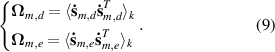
Denoting the first Rm rows of W m and the rest as W m,d (Rm × J) and W m,e ((J−Rm ) × J), respectively, multiple static models are constructed for different flow regimes by performing SFA [23]
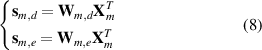
where s m,d refers to the derived slowest features that tend to catch the general trend of process variations in the mth flow regime; s m,e represents the fastest features, which can be seen as short-term noises or fluctuations.
Step 3: Establish local models to monitor dynamics.
Because the slow features vary slowly and reflect the overall steady-state distribution, the derivative of the slow features can reflect the changing trend and dynamic characteristics of the flow statuses. The first-order derivatives of the slow features are considered to detect process dynamics. Multiple dynamic models are constructed for different flow regimes based on  and
and 
Step 4: Calculate statistics and control limits.
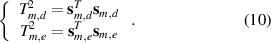
To measure the static variations of flow status, the T2 statistics of the mth model are defined based on s m,d and s m,e
Because of the non-Gaussian distribution of the slow features in SFA, the control limits of the T2 statistics in the mth status,  and
and  , are calculated using kernel density estimation (KDE) [21]. The confidence level is chosen as α= 0.99 in this work. The T2 statistics reflect whether the current status conforms to the model.
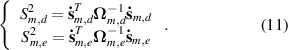
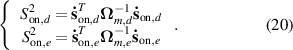
To detect process dynamics, two S2 statistics are defined based on  and
and  :
:
The control limits in the mth flow regime,  and
and  , are also calculated using KDE. The S2 statistics reflect whether the dynamics of the current status and the corresponding model status are consistent.
2.3. Bayesian inference-based online identification for flow status
In status identification, Bayesian inference is developed using the T2 static statistics to obtain an intuitive index for identifying the current flow status, while the S2 dynamic statistics are used to detect process dynamics. The online status identification and analysis steps are summarized as follows:
Step 1: Collect the real-time data xon, and then normalize the data to get 
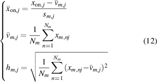
where xon,j
is the online sampling data for the jth process variable. The mean and the standard deviation of the jth process variable in the mth modeling data matrix are represented by  and hm,j
, respectively.
and hm,j
, respectively.
Step 2: The slow features are obtained by projecting  onto the local model W
m:
onto the local model W
m:
Step 3: Calculate the T2 online monitoring statistics.
The two statistics are used to measure whether the current status corresponds to the status of the mth model. If either of them (or both) exceeds its control limit, this indicates that the status of gas–liquid two-phase flow has changed.
Step 4: Bayesian inference is developed using the T2 statistics.
Here, the two T2 statistics and the two control limits are combined to provide an intuitive and comprehensive index of the process status [26]. The event of the mth typical flow regime is represented by Lm
. In the Bayesian inference of this work, the within-class conditional probability of xon with respect to  is computed as:
Correspondingly, the without-class conditional probability of xon with respect to  is computed as
The posterior probability is then defined as the identification index
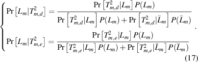
As described above, s d represents the main information, which catches the general trend of process variations; s e represents residuals with fast variations and contains very little information. Therefore, the two probabilities in formula (17) are given different weights

where λ (0.5 < λ < 1) and (1 − λ) are the weights assigned to ![$Pr[{L_m}|T_{m,d}^2]$](https://content.cld.iop.org/journals/0957-0233/32/5/055301/revision3/mstabdae4ieqn23.gif) and
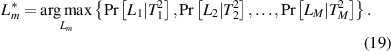
and ![$Pr[{L_m}|T_{m,e}^2]$](https://content.cld.iop.org/journals/0957-0233/32/5/055301/revision3/mstabdae4ieqn24.gif) , respectively (λ is set as 0.8 in this work). The current flow status is then assigned to the status with the largest identification index
, respectively (λ is set as 0.8 in this work). The current flow status is then assigned to the status with the largest identification index ![$Pr[{L_m}|T_m^2]$](https://content.cld.iop.org/journals/0957-0233/32/5/055301/revision3/mstabdae4ieqn25.gif)
Step 5: Calculate the S2 online monitoring statistics.
The two statistics are used to measure consistency with the process dynamics. Once either of them (or both) exceeds its threshold, the dynamic characteristics of the current process do not correspond to the model.
The concurrent modeling and identification strategy for the steady states and process dynamics is shown in figure 1. The four possible results and descriptions are listed in table 1.
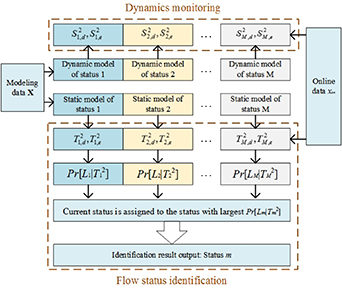
Figure 1. Modeling and identification strategy.
Download figure:
Standard image High-resolution imageTable 1. Process status as indicated by monitoring statistics.
| Case |


|


| Process status |
|---|---|---|---|
| 1 | √ | √ | Process is in the flow status corresponding to the model |
| 2 | √ | × | Process is in the flow status corresponding to the model, but some different dynamic characteristics are detected |
| 3 | × | √ | Process is not in the flow status corresponding to the model but has some similar dynamic characteristics |
| 4 | × | × | Process is not in the flow status corresponding to the model |
('√' refers to the situation whereby both statistics are within control limits;'×' refers to the situation whereby one or both statistics are outside control limits)
3. Experiments with a gas–liquid two-phase flow
3.1. Modeling data selection
In gas–liquid two-phase flow processes, the flow status is closely related to the pressure at the pipe inlet, the temperature, the velocity of each phase fluid, the medium distribution, and the phase holdup. The sensors used to measure gas-water two-phase flow are shown in table 2.
Table 2. Sensors for measuring gas-water two-phase flow.
| Sensors | Fluid characteristics | Associated flow parameters |
|---|---|---|
| Conductance | Electrical conductivity | Phase holdup |
| Capacitance | Dielectric constant | Phase holdup |
| Continuous wave ultrasonic Doppler | Density | Flow velocity |
| Pressure | Pressure | Manifold pressure |
| Resistance Array | Resistance | Phase medium distribution |
A conductance sensor is composed of six ring electrodes, and the potential difference is measured between each pair of electrodes. In the experiments, changes to the flow structure lead to changes in the mixture's conductivity and cause changes in electric potential difference. Therefore, the potential difference can be used to calculate the water holdup [7]. The measurement data from the conductance sensor are preprocessed according to formula (21) and selected as modeling data, which reflect the phase holdup information of the gas–liquid two-phase flow when the conductive phase is continuous.
where Vw denotes the value when the tube is filled with water, Vmeas denotes the actual measurement data, and Vn denotes the normalized voltage that reflects phase holdup.
A capacitive sensor consists of two electrode plates. The dielectric constant of the mixed fluid is determined by the dielectric constants of each phase and the phase distribution. There is a corresponding relation between the measured capacitance and phase holdup [8]. The measurement data of the capacitive sensor are selected as modeling data to reflect the phase holdup information when the non-conductive phase is continuous. They are complementary to the data of the conductance sensor. These data are preprocessed according to formula (22)
where RCD denotes the relative change of capacitance and Vmeas, VI, and Vw denote the voltage of the fluid, the voltage when the pipe is filled with non-conductive phase, and the voltage when the pipe is filled with water, respectively.
The transmitting piezoelectric chip (TPC) of a continuous-wave ultrasonic Doppler (CWUD) sensor emits a continuous sinusoidal ultrasonic wave, and the receiving piezoelectric chip (RPC) receives the wave reflected by dispersed phase droplets. According to the Doppler effect, the average Doppler shift and the average velocity of the dispersed phase in the sample volume are obtained by calculating the Doppler shift of the ultrasonic signal between the TPC and RPC [27]. The Doppler shift data of the CWUD sensor are selected as modeling data to reflect the flow velocity information.
A pressure gauge is installed at the inlet of the horizontal pipe to measure the pressure at the pipe's inlet. The pressure data are selected as the modeling data that mainly reflect the flow environment information.
A resistance array consists of 16 electrodes and provides two-dimensional medium distribution information for the two-phase flow. The boundary voltage data of the different electrodes are preprocessed [28] according to formula (23) and selected as modeling data.
where Vij represents the jth (j= 1, 2, ..., n) boundary voltage measured in the ith (i= 1, 2, ..., 16) excitation direction, Vij 0 represents the jth boundary voltage measured in the ith excitation direction on the condition that the pipe is full of water, and VRi represents the characteristic value of boundary voltages in the ith excitation direction.
Since the ambient temperature changes very little and has little influence on the gas–liquid two-phase flow process, the temperature is not selected.
3.2. Experimental data acquisition
The experimental data are collected from a horizontal pipe of the gas–liquid two phase flow loop. The experimental device and test section are shown in figure 2. In the experiments, the different flow ratios of each phase are adjusted to form various flow statuses within the experimental device. The experimental data are then obtained and multiple SFA-based local models can be established.

Figure 2. Gas–liquid two-phase flow loop.
Download figure:
Standard image High-resolution imageIn the experiments, the liquid phase is tap water (with a density of 998 kg m−3 and a dynamic viscosity of 1.01 × 10⁻³ Pa•s) and the gas phase is dry air (with a density 1.2 kg m−3 and a dynamic viscosity of 1.81 × 10⁻⁵ Pa•s). The horizontal pipe made of stainless steel is 16.6 m in total length with an inner diameter of 50 mm. Standard single-phase flow meters are used to measure each phase in front of the mixer inlet. The test section where the combined sensors are installed is located 12 m downstream from the inlet to allow the flow status to fully develop. A camera is used to directly observe and record the flow status. Besides, the pressure gauge and temperature gauge are installed to monitor the flow environment. By controlling the flow rate of the gas and liquid before they reach the mixer, six typical flow regimes and transition statuses are formed, namely, bubble flow, plug flow, slug flow, wave flow, stratified flow, and annular flow [29].
Data acquisition is carried out for the six typical flow regimes and transition statuses between different flow regimes. The collection time of each data set is 10 s. The acquisition frequencies of the conductance sensor, capacitance sensor and pressure gauge are 2 kHz, and the acquisition frequency of the CWUD sensor is 50 kHz. Two thousand eight hundred frames of data can be measured by the resistance array sensor in 10 s. In this way, a set of two-dimensional data can be obtained every 10 s. Each set includes three voltage data columns from the conductance sensor, two voltage data columns from the capacitance sensor, one Doppler shift data column from the CWUD sensor, one voltage data column from the pressure gauge, and 16 data columns from the resistance array sensor. The data have to be resampled to realize time matching because of inconsistent sampling frequencies. After resampling and preprocessing, each data set is collected as a two-dimensional data array Y(2800 × 23). For each typical flow regime, three sets of data are used for modeling, and two sets of data are reserved as test data.
3.3. Offline modeling for typical flow regimes
Based on the modeling data of the gas–liquid two-phase flow, six typical flow regimes are modeled according to the method presented in section 2. The coefficient matrices W m,d , W m,e and the diagonal matrices Ω m,d , Ω m,e are obtained as model matrices. Besides, the control limits for each model are calculated. The first four slow features extracted for each typical flow regime are presented in figure 3.

Figure 3. Slow features of typical flow regimes.
Download figure:
Standard image High-resolution imageFigure 3 suggests that the slow features of typical flow regimes are different and represent the inherent essential properties, which provides a theoretical basis for the status identification of the two-phase flow process based on multiple slow feature analysis. Five hundred sampling points of each flow regime are used for verification, and the results are shown in figure 4. Four statistics stay below the control limits for most of the sampling points, verifying the validity and accuracy of the models.
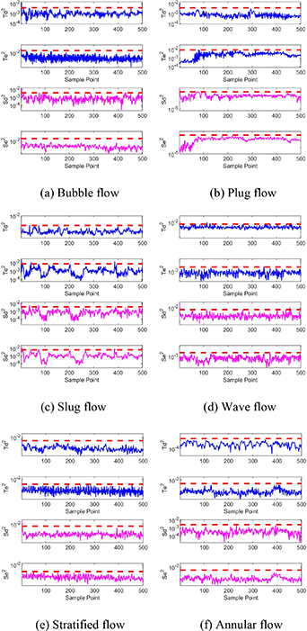
Figure 4. Verification of models of the typical flow regimes.
Download figure:
Standard image High-resolution image4. Flow status identification results and analysis
4.1. Identification for typical flow regimes
During online status identification, the data should be collected continuously in real time. Moreover, in the two-phase flow in an actual industrial process, the most common flow regimes are bubble flow, plug flow and slug flow. In the experiment, the amounts of data for each flow regime are also different. Considering the flow regimes of two-phase flow in actual industrial processes and the amounts of data for each flow regime obtained in the experiment, the test sample is set up as follows: the first ∼400 sampling points are in bubble flow, sampling points 401 ∼ 900 are in plug flow, sampling points 901 ∼ 1300 are in slug flow, sampling points 1301 ∼ 1600 are in wave flow, sampling points 1601 ∼ 1900 are in stratified flow, and sampling points 1901 ∼ 2200 are in annular flow. Bayesian inference is developed to obtain an intuitive identification index. For the PCA and ICA methods, according to minimum squared prediction error (SPE) [30], the SPE statistics are used to calculate Bayesian inference-based indexes. The identification results from the multiple PCA method, the multiple ICA method and the proposed method are presented in figures 5–7, respectively.
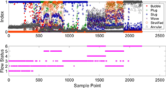
Figure 5. Multiple PCA-based identification indexes and results for typical flow regimes.
Download figure:
Standard image High-resolution image
Figure 6. Multiple ICA-based identification indexes and results for typical flow regimes.
Download figure:
Standard image High-resolution image
Figure 7. Multiple SFA-based identification indexes and results for typical flow regimes.
Download figure:
Standard image High-resolution imageIn figures 5–7, flow statuses one, two, three, four, five and six on the vertical axis of the figures respectively denote bubble flow, plug flow, slug flow, wave flow, stratified flow and annular flow. The multiple SFA method has the highest accuracy among the three methods. In general, the flow status identification results using the proposed method are satisfied, with an overall false identification rate of 1.64%. The false identification rates for different flow regimes of the three methods are presented in table 3.
Table 3. False identification rates of the three methods.
| Flow status | PCA | ICA | SFA |
|---|---|---|---|
| Bubble flow | 66.75% | 4.50% | 6.75% |
| Plug flow | 31.80% | 19.20% | 1.40% |
| Slug flow | 0.50% | 0% | 0% |
| Wave flow | 56.30% | 0.33% | 0% |
| Stratified flow | 31.00% | 1.00% | 0.67% |
| Annular flow | 1.00% | 0% | 0% |
| Overall | 31.50% | 5.36% | 1.64% |
For the multiple PCA method, the false identification rate is high for all the flow statuses except for slug flow and annular flow. Taking the first 400 sampling points, for example, numerous sampling points are misidentified as plug flow and slug flow (as in figure 5). The detailed monitoring statistics are shown in figure 8, which represent the monitoring results using the slug flow model.

Figure 8. Monitoring results using the PCA-based model of slug flow.
Download figure:
Standard image High-resolution imageIn figure 8, the T2 statistics are below the control limit for almost all of the first 1300 sampling points, indicating that there is no change of flow status. Therefore, the T2 statistics barely detect the change of status before the one thousand three hundredth sampling point. Meanwhile, SPE statistics cannot distinguish bubble flow from slug flow. After Bayesian inference, the identification result from the multiple PCA method is disappointing.
For the multiple ICA method, the false identification rate is high for plug flow (as shown in figure 6). To analyze the identification results more meticulously, monitoring statistics using the models of plug flow and slug flow are shown in figures 9 and 10, respectively.
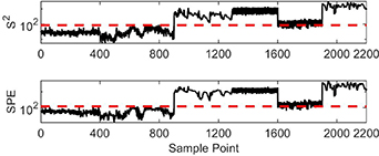
Figure 9. Monitoring results using the ICA-based model of plug flow.
Download figure:
Standard image High-resolution image
Figure 10. Monitoring results using the ICA-based model of slug flow.
Download figure:
Standard image High-resolution imageIn figure 9, none of the two statistics in the first 400 sampling points exceed the control limit, and some of them are even smaller than those of the four hundred and first to nine hundredth sampling points. This implies that the change of status from bubble flow to plug flow cannot be detected. In figure 10, it can be seen that the monitoring results from ICA are better than those of PCA (as shown in figure 8). However, two statistics are below the control limits for some sampling points in the four hundred and first to nine hundredth sampling points, which means that some sampling points in the plug flow are misidentified as being in slug flow.
The process of multiphase flow tends to be dynamic, that is, process data are associated with time. However, PCA and ICA assume that process data are statically independent, causing the dynamics of the process to be ignored. This means that it is difficult to accurately describe the actual variations of the data, and therefore, the identification effect is not ideal.
For the multiple SFA method, some sampling points in the bubble flow are misidentified as plug flow (as in figure 7). Monitoring statistics are used to analyze the flow process in the first 900 sampling points more meticulously and monitor the process dynamics. The monitoring results using the multiple SFA-based models for bubble flow and plug flow are shown in figures 11 and 12, respectively.

Figure 11. Monitoring results using the SFA-based model for bubble flow.
Download figure:
Standard image High-resolution image
Figure 12. Monitoring results using the SFA-based model for plug flow.
Download figure:
Standard image High-resolution imageIn the plot of figure 11(a), the T2 statistics detect the change of flow status after the four hundred and first sampling point. In the plot of figure 11(b), from the four hundred and first to the one thousand three hundredth sampling points, a few of the  and
and  statistics are below the control limits. This indicates that although the status has changed, there are still some similar dynamic characteristics. In figures 12(a) and (b), the monitoring results of the SFA are better than those of ICA (as in figure 9). The
  statistics that capture the main variations are around the control limit before the four hundredth sampling point, and they are higher than those of the four hundred and first to eight hundredth sampling points; some of them exceed the control limit. The S2 statistics reveal some similarity of dynamic characteristics between bubble flow, plug flow, and slug flow. Because there are small bubbles in plug flow and slug flow, the flow process exhibits similar properties at certain periods. The monitoring results show that the proposed method can not only identify typical flow regimes but also accurately detects similar dynamic characteristics in different flow statuses.
4.2. Identification and analysis for transition flow status
In gas–liquid two-phase flow processes, the transition statuses between different flow regimes are common and important, have an important influence on the flow process, and should be paid attention to. The experimental data of the transition status from bubble flow to slug flow (as shown in figure 13) are used for testing. The first stage contains 500 sampling points in bubble flow. The second stage contains three data sets representing the transition of the flow status from bubble flow to slug flow, each with 200 sampling points. The third stage contains 500 sampling points in slug flow. In the experiment, the change from bubble flow to slug flow is the result of an increase in the gas flow rate.
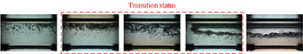
Figure 13. Photos of the transition from bubble flow to slug flow.
Download figure:
Standard image High-resolution imageBayesian inference is developed to identify the flow status. Because the flow process fluctuates complexly and violently in the transition status, a time sliding window L is used to smooth the Bayesian inference-based index. The transition status and typical flow regimes can then be identified by the following criteria:
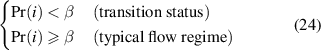
where Pr(i) denotes the Bayesian inference-based index of bubble flow or slug flow, and β (0 < β< 1) is the threshold (β is set to 0.5 in this work).
The identification results using multiple SFA combined with Bayesian inference are shown in figure 14.
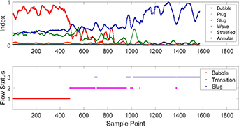
Figure 14. Identification results for transition status using the multiple SFA combined with Bayesian inference.
Download figure:
Standard image High-resolution imageIn the plot of figure 14, flow statuses one, two and three respectively denote bubble flow, transition, and slug flow. It can be seen that the Bayesian inference-based index of bubble flow has a decreasing tendency, while that of slug flow has an increasing tendency. The transition status is from the four hundred and eighty-fifth to the one thousand and fourteenth sampling points.
To monitor the steady states and process dynamics of the changing process accurately and meticulously, statistics are used for analysis. Two other methods are compared with the proposed method. The distributions of statistics using the three methods are shown in figures 15–17, respectively.
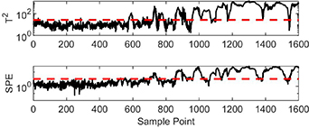
Figure 15. Monitoring results fromom multiple PCA.
Download figure:
Standard image High-resolution image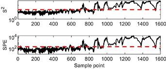
Figure 16. Monitoring results from multiple ICA.
Download figure:
Standard image High-resolution image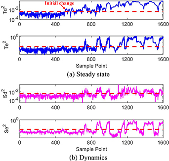
Figure 17. Monitoring results using the multiple SFA.
Download figure:
Standard image High-resolution image
In the plot of figure 15, the T2 statistics cause false alarms at the thirtieth and the two hundred and eighty-sixth sampling points. From the five hundred and first to the seven hundredth sampling points, a few of the T2 and SPE statistics exceed the control limits, while there are still many statistics below the control limits. This indicates that the flow status of the process is changing. From the seven hundred and first to the thousandth sampling points, numerous T2 and SPE statistics are outside the control limits, while there are a few statistics below the control limits, indicating that the current process is in transition status and has both bubble flow characteristics and slug flow characteristics. After the one thousand and first sampling point, both indexes exceed the control limits for most of the sampling points, indicating a complete change in flow status. In practice, the fluid is mixed with numerous small bubbles in slug status. However, the principal component information extracted by PCA only shows that there is a change in status, with no more information provided.
In the plot of figure 16, the S2 and SPE statistics indicate the process is in bubble flow for the first 500 sampling points. As opposed to the results from multiple PCA, both statistics seldom exceed the control limits during the five hundred and first to seven hundredth sampling points, in which the initial change has been ignored. After the seven hundred and first sampling point, the distribution of statistics is similar to that using multiple PCA method. The monitoring results of the above two methods lead to the same conclusion, which is that they can identify the process status, but they cannot distinguish the dynamic potential changing trend or the similar dynamic characteristics among different flow statuses.
In the plot of figure 17, the steady states monitored by  and
and  are illustrated in figure 17(a), and the process dynamics described by
  and
and  are plotted in figure 17(b). There is an increasing tendency in the statistics. Two of the T2 statistics stay below the control limits for the first 500 sampling points, illustrating that the flow status is bubble flow, while the process appears to operate around the control limit of
  . The
. The  statistics exceed the control limit at around the fifty-first, the two hundred and thirty-ninth and the three hundred and ninety-ninth sampling points, indicating that the dynamic variation has been noticed before the transition status. From the five hundred and first to the seven hundredth sampling points, a few
  statistics exceeding the control limits detect the initial change, which is earlier than PCA and ICA. However, the S2 statistics remain similar to the distribution of the first 500 sampling points, which indicates that although the status is changing, the dynamic characteristics of the current process have not changed much and the process is in the initial stage of transition status. This similarity can be seen in the first two photos in figure 13; small bubbles gradually coalesce into larger ones. From the seven hundred and first to the thousandth sampling points, the T2 and S2 statistics exceed the control limits for some sampling points, while there are still some statistics under the control limits, illustrating that the process is in transition status. After the one thousand and first sampling point, the two T2 statistics exceed the control limits for most of the sampling points, indicating that the flow status has changed completely to slug flow. Some of the S2 statistics are still below the control limits because of the similar dynamic characteristics of bubble flow and slug flow.
From the above analysis, PCA and ICA can only tell whether the change of flow status has been detected but cannot provide dynamic information or detect similar characteristics in different flow statuses. The flow status changes over time, so the dynamic characteristics of the time-varying flow process should be fully considered. Moreover, although there are great differences among the flow statuses of a gas–liquid two-phase flow, there are still some similarities in finite time that should not be ignored. Unlike PCA or ICA, the proposed method provides more meaningful information by concurrently monitoring both the steady states and the process dynamics. SFA extracts information of two characteristics, which are the slow features and the first-order derivative of the slow features. The information extracted by SFA is more comprehensive and the physical significance is clearer. Therefore, the identification and analysis made by SFA are more in line with the actual situation and have better interpretability.
5. Conclusions
A method based on multiple SFA was proposed, aimed at solving the problem of the status identification of a gas–liquid two-phase flow process in a horizontal pipe. This status identification method used the idea of status monitoring. The flow measurement data obtained from multiple sensors were utilized to extract the slow features and the first-order derivative of the slow features. Multiple SFA-based local models were then constructed to describe both static and dynamic process information for different flow statuses, respectively. Bayesian inference was designed as an intuitive index to identify flow status during online identification. In comparison with the PCA and ICA methods, the multiple SFA flow process identification scheme was not only able to detect the change of flow status by monitoring the steady distribution but was also able to detect process dynamics according to the changing trends of slow features. This provided more meaningful information to better understand the flow process. In the experiments, various flow statuses were formed using a gas–liquid two-phase flow experimental apparatus, and multiple sensors were used to obtain measurement data. The feasibility and efficiency of the proposed method were validated using the test data.
Acknowledgments
The authors gratefully acknowledge support from the following foundations: the National Natural Science Foundation of China (51976137 and 61903272), and the Natural Science Foundation of Tianjin (19JCZDJC38900 and 20JCQNJC01670).