

Abstract
The long-term condition and potential radiological consequences of legacy radioactive waste stored in a RADON-type of near-surface disposal facility outside the city of Chişinău is of concern to the central government and health protection authorities of the Republic of Moldova. A 'zero alternative scenario' risk assessment has been undertaken in order to evaluate the potential radiological impact on humans and the environment of the facility, were it to be left in its current state with no remediation. The results have been used as a basis for regulatory decision making regarding remediation and decommissioning of the legacy radioactive waste facility. The aim of this study was two-fold: first to demonstrate a complete radiological risk assessment of a real site using a combination of methodologies developed by the IAEA (ISAM and BIOMASS), the second to illustrate the current state-of-the-art in respect of extracting site-specific information from site-descriptive material. We illustrate the practicality of employing geographic information systems techniques on site-specific topographic data to identify relevant biosphere dose objects, thereby allowing customisation of the generic ISAM model framework to site-specific conditions. As a result, a simple method is suggested to bound activity concentrations in well water based on an understanding of water balance in the local catchment area in which the biosphere dose object is embedded. With conservative assumptions, estimated doses from the calculation cases of the design scenario remain lower than the IAEA's dose criteria and environmental screening values. However, the results also indicate that human intrusion activities after the institutional control period could lead to radiological exposures above the IAEA's criteria for a period up to 100 000 years. The long-lived radionuclide 239Pu dominates doses for the on-site residence scenario. Remediation measures should be implemented were the waste to remain at its present place of disposal.
Export citation and abstract BibTeX RIS

Original content from this work may be used under the terms of the Creative Commons Attribution 4.0 license. Any further distribution of this work must maintain attribution to the author(s) and the title of the work, journal citation and DOI.
1. Introduction
The Republic of Moldova has a legacy of low-level radioactive waste from the Soviet era in the form of radioactive sources and radioactive waste. One such waste management challenge is a RADON-type near-surface disposal facility not far from, and upstream of, the capitol city, Chişinău. Within the framework of Sweden's bilateral support programme, the Swedish Radiation Safety Authority (SSM) has financed a radiological risk assessment for this waste facility with the objective of assessing potential radiological impact on humans and the environment assuming that no remediation is implemented (the zero alternative case). An important rationale for conducting the assessment is also to provide a basis for regulatory decision making regarding possible decommissioning of the disposal facility.
The project comprised two parts. The first was the development of a site-descriptive model for the near-surface disposal facility and its surroundings that serves as a basis for developing a radiological safety assessment (Anton 2017, Dimo and Mosoi 2018, Bogdevici 2019). The second was a radiological risk assessment of a zero alternative case for the disposal facility (Xu and Kłos 2019, 2021).
In performing the assessment we combine two methodologies developed by the IAEA: ISAM (IAEA 2004a) and BIOMASS and its update (IAEA 2003a, 2020). ISAM sets out the steps needed to define the structure of the assessment and is used to identify the scenarios to be addressed. One ISAM example specifically addresses the RADON-type facility, simplifying the identification of scenarios and mathematical models applied here (IAEA 2004b). However, the ISAM case is a more generic illustrative example combining features and data from different sites around the world. We use the updated BIOMASS methodology (IAEA 2020) to customise the assessment model structures and datasets based on the site-descriptive material available from the first stage of the assessment. In particular we define a biosphere dose model from the original ISAM conceptual model expressed as an interaction matrix by applying the approach of Kłos and Thorne (2020) using site-specific detail.
Customisation of the biosphere and dose submodels makes use of site-specific details in the digital elevation model of the site using geographic information systems (GIS) techniques to provide visualisation of the site and to extract numerical data (Guerfi et al 2019). This allows us to identify the main watershed areas around the site and to define suitable areas for dose assessment purposes. A dynamic soil model for the dose assessment has been developed on this basis and results from this are compared with the equilibrium soil model used in the initial assessment of the site (Xu and Kłos 2019).
The issue of dilution in the aquifer is a well-known problem in such dose assessments. In generic repository safety assessment, the dose rate is highly sensitive to the dilution in the aquifer, however, the quantification of dilution is sometimes set at an arbitrary value (IAEA 2003a). There are various methods for describing the dilution of contaminants in groundwater following leakage from a waste source to a well (e.g. Naturvårdsverket 2009, Mariner 2013). Here we take a simple approach, using the overall water balance in the local watershed area associated with the biosphere object in which doses are assumed to occur. In this way we avoid difficulties in defining the dilution factor which can change by orders of magnitude over time due to changes in the advective flux to the aquifer (Mariner 2013). The method we use allows the dilution in the aquifer to be bounded based on the geometrical considerations of the landscape and the requirements of the radiological assessment model.
The legal framework in the field of radioactive waste management in Moldova is currently under development, which is why, for the time being, there is no national regulatory guidance for undertaking risk assessments for near-surface disposal facilities. This radiological risk assessment is therefore based on international standards and best practice.
2. Method
2.1. Overview of the combined assessment methodologies
The RADON-type waste facility is a near-surface design common in the Soviet Union during the latter 20th century for radionuclides arising from non-nuclear fuel cycle sources. The ISAM reports (IAEA 2004a, 2004b) document the assessment of such hypothetical facilities similar in concept to the existing facility at Chişinău. The methodology for the assessment consists of the following main steps:
- (i)specification of the assessment context,
- (ii)description of the waste disposal system,
- (iii)development and justification of scenarios,
- (iv)formulation and implementation of models, and
- (v)analysis of results and confidence building.
With specific reference to the characterisation of the biosphere, elements of BIOMASS (IAEA 2020) are applied at stage iv.
2.2. Assessment context
The objective of this radiological risk assessment is to provide a basis for regulatory decision making regarding decommissioning of the legacy radioactive waste at the RADON-type facility at Chişinău. The assessment endpoints are annual effective doses to the assumed human inhabitants of the selected biosphere location and environmental concentrations used to assess the potential radiological impact on non-human biota. The calculated annual effective doses are compared with the specific criteria given in IAEA SSR-5 (IAEA 2011) and environmental concentrations are compared with environmental media concentration limits (EMCLs) (Brown et al 2016).
The initial inventory (table 1) was used to determine the timescale for the assessment using the radiotoxicity of the waste, calculated as the committed effective dose from ingestion of the radionuclides directly and expressed as a percentage related to the total radiotoxicity at closure. Long-lived 239Pu dominates the radiotoxicity (figure 1), which falls to around 10% of the initial value after around 100 kyear. This is the upper limit of the dose assessment time period and the starting time assumes an institutional control period of 300 years, as is common for this type of assessment (IAEA 2004a).
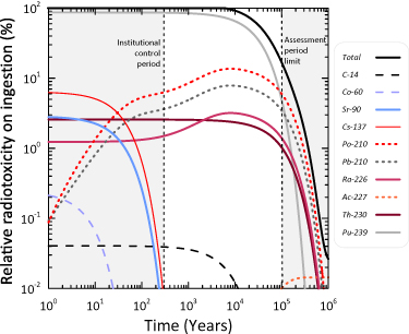
Figure 1. Percentage contribution to total radioactivity as a function of time. Radionuclides with greater than 0.1% of the toxicity at any time are shown. Numerical assessment runs from the end of the institutional control period at 300 years to 100 kyear.
Download figure:
Standard image High-resolution imageTable 1. Initial activity inventory and half-lives of radionuclides in the repository including key progenies that grow-in over time (modified based on Anton 2017). Reproduced with permission from Anton (2017).
| Radionuclide | Disposed inventory (GBq) | Half-life (year) |
|---|---|---|
| 3H | 0.491 | 12.3 |
| 14C | 48.6 | 5.73 × 10³ |
| 36Cl | 3.7 × 10⁻² | 3.01 × 10⁵ |
| 60Co | 49.6 | 5.27 |
| 63Ni | 3.07 × 10⁻⁵ | 100.1 |
| 85Kr | 2.41 | 10.8 |
| 90Sr | 64.8 | 28.8 |
| 137Cs | 341.0 | 30.1 |
| 204Tl | 5.79 × 10⁻⁴ | 3.78 |
| 226Ra | 3.05 | 7.54 × 10⁴ |
| 230Th | 8.51 | 2.41 × 10⁴ |
| 239Pu | 241.0 | 12.3 |
| 210Po | 0.0 | 0.379 |
| 210Pb | 0.0 | 22.3 |
| 227Ac | 0.0 | 21.8 |
| 231Pa | 0.0 | 3.28 × 10⁴ |
| 235U | 0.0 | 7.04 × 10⁸ |
2.3. Site-description and regional characteristics
2.3.1. Waste disposal facility.
The facility consists of four reinforced concrete vaults (numbered I to IV), with total area around 80 m2. The vaults are configured as shown in figure 2 with each having an openable lid for loading and to provide access. The size of the opening is about 700 × 1200 mm and although the internal volume of each of the four vaults is 42, 45, 36 and 42 m3, giving a total capacity of about 165 m3, the size and position of the openings means that the vaults cannot be filled completely. Waste was simply dropped through the opening with no special placement measures. The total volume occupied by the disposed waste is therefore about 75 m3. Records of the disposed waste packages characterise them as unstable waste form, stable waste form, or disused sealed radiation source. All details are taken from Anton (2017).
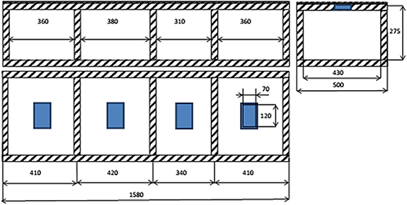
Figure 2. Vault layout and cross section (Anton 2017). Blue rectangle indicates position of the loading aperture. Dimensions are shown in centimetres. Reproduced with permission from Anton (2017).
Download figure:
Standard image High-resolution imageSince construction of the facility the concrete structures of the vaults have been open to the elements and none of the four vaults provide satisfactory isolation (see figure 3). According to the operator's description an elevated groundwater table was observed inside Vault IV during the late 1990s. 90Sr and 226Ra were detected in soil and groundwater in the vicinity of the disposal facility by the National Centre of Preventive Medicine in 1998 (NCPM 1998).

Figure 3. Condition of the facility showing evidence of weathering of the concrete structures (Anton 2017). Reproduced with permission from Anton (2017).
Download figure:
Standard image High-resolution image2.3.2. Landscape and climate.
The near-surface disposal facility is located in the Chişinău municipality, and the terrain adjacent to the facility (area 455 ha) falls within the city limits (figure 4). The location of the disposal facility is shown bordered by the white boundary and the area that defines the landscape context, local to the site, by the red boundary.
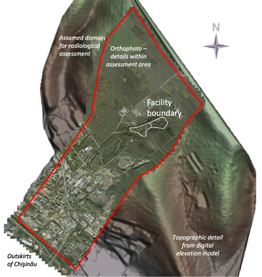
Figure 4. Map of the site. The location of the disposal facility is shown bordered by the white boundary. The area of the orthophoto is shown overlain on the topographic map. The red boundary denotes the area for the overall radiological assessment model. Reproduced with permission from Dimo and Mosoi (2018).
Download figure:
Standard image High-resolution imageBogdevici (2019) reports the hydrogeological and geotechnical conditions at the site, as well as providing the digital elevation model for the site. The facility is located in a small valley ranging in elevation from 81 to 118 m with the upper elevations of the landscape around 130 m. In the valley, around the facility, local slopes are more than 6° but at the higher elevations the slopes are in the range 3°–6°.
The upper part of geological section is characterised by shallow thicknesses of Quaternary loam and Neogene sandy-clay formations. These are covered by agricultural and artificial soils. The Neogene formation comprises sandy loam layered with clay and clay layered with sands. The upper parts of the clays, located at slopes with high inclination, are intensively fractured. This clay is dense, dry, semi-dry, and fractured, with fine sand layers and carbonate inclusions. Groundwater can form seasonally at shallow depths due to the presence of clays at depths of 3–4 m.
Climate records have been maintained in the Republic of Moldova since 1886 and continue via the monitoring network of the State Hydrometeorological Service (Anton 2017). Current meteorological monitoring at the disposal site indicates an average precipitation of 573 mm yr−1 with maximum 744 mm yr−1 and minimum 425 mm yr−1. Evapotranspiration in the vegetated areas is assessed as 80% of precipitation.
Projections of future climate conditions for the Republic of Moldova suggest that what are currently considered to be extreme rare events for absolute maximum temperatures (around 35 °C for the baseline period of 1961–1990) are likely to become mean maximum summer temperatures. Projections for Europe more generally indicate that the risk of floods increases in Northern, Central and Eastern Europe and that today's 100 year droughts will return every 50 years especially in Southern and South-Eastern Europe, including in the Republic of Moldova (Lehner et al 2006). The probability of flooding, particularly in the valley around the facility, is therefore expected to increase.
The general characterisation of land use around the site (figure 5) shows the dominance of infrastructure land (42.8% of the total area) mostly at lower elevations, towards the city boundary. Agricultural land is currently 38.1% and non-agricultural natural ecosystems 19.1%. Commercial arable production occupies 59.2% of the cultivated area, with individual plots a further 2.7%. Fruit cultivation (16.6%) and a small amount of grassland (2.5%) are also present. The land classified as non-agricultural just downslope from the facility could be suitable for cultivation as there is currently some cultivation adjacent to the facility boundary.
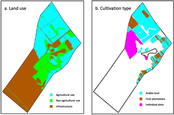
Figure 5. Land use map classification (Dimo and Mosoi 2018).
Download figure:
Standard image High-resolution image2.4. Development and justification of scenarios for radiological assessment
Scenarios are considered as a hypothetical sequence of features, events and processes (FEPs) intended for the purpose evaluating safety by exploring range of possibilities that could lead to radiation exposures for inhabitants of the modelled area. They are intended to portray alternative future states of the system in a systematic and managed way on timescales suited to the assessment context. IAEA (2004a, 2011, 2012, 2014) classifies scenarios for radiological assessment purposes as:
- The base scenario—also known as the reference scenario, expected evolution, normal evolution or undisturbed performance,
- Alternative scenarios—scenarios that may deviate from the reference evolution of the disposal facility or which may represent rare or unlikely situations,
- Human intrusion scenarios—carried out on the basis of more stylised descriptions that have been agreed with the regulatory body and address specific concerns, and
- What-if scenarios—often intended to illustrate the specific properties of one or more of the natural or engineered barriers.
FEP screening for the RADON Test case in the ISAM report (IAEA 2004a) identifies three groups of scenarios: undisturbed performance, naturally disturbed performance and inadvertent intrusion. Each of these should be addressed for both on-site and off-site human residence. Combining these scenarios with the required FEPs generates a set of general scenarios. The ISAM test case therefore greatly simplifies the procedure for deriving scenarios in this study. Site-specific detail can further be used to filter the FEPs so as to configure the resultant models closely to site conditions. The selected scenarios and calculational cases are set out below. In this assessment we have not assessed What-if cases.
2.4.1. Design scenario.
The design scenario (ISAM SCE1, also called reference evolution) is based on the probable evolution of the system in respect of external conditions combined with realistic or, where justified, pessimistic assumptions with respect to internal conditions.
The disposal facility is located at a relatively high elevation so that it can be expected to be part of a groundwater recharge area. Design scenario, SCE1 with the initial state that the engineered barrier is partly degraded, is selected and a small farm assumed to be located at the disposal facility boundary. This design scenario is a relevant type of normal evolution scenario. The use of a farm system ensures that a comprehensive range of exposure pathways is assessed, maximising human interactions with potentially contaminated material. As described in section 2.5, the site context here suggests well water as the most likely source of drinking and domestic water supplies as well as for irrigation of cultivated land.
2.4.2. Alternative scenarios.
Scenarios that may deviate from the reference evolution for the long-term safety of the disposal facility are selected as alternative scenarios. Since the main safety function for the existing facility is provided by the concrete walls of the vault, possible routes to violation of the safety function are used to identify the alternative scenarios.
The frequency of flooding is expected to increase in line with the climate predictions outlined in section 2.3.2, so we select flooding and associated landslides as alternative scenarios. Anton (2017) notes that today's 100 year droughts in Europe are likely to occur on timescales of 50 years the cumulative frequency of this rare event,  can be written as:

in which  is time (year AP). No frequency function is assigned to the landslide scenario.
2.4.3. Human intrusion scenarios.
Two human intrusion scenarios are also selected based on figure B-1in the ISAM report (IAEA 2004a) to assess the disturbed evolution of the disposal facility:
- (a)on-site residence scenario (SCE6), and
- (b)the road construction scenario (SCE7), used to assess risks to humans intruding into the disposal facility after institutional control.
2.5. Identification of the biosphere dose object
A biosphere dose object may be simply defined as a location in the biosphere where human activities can be assumed to lead to exposure to radionuclides in environmental media.
The ISAM example (IAEA 2004b) considers both well and river water sources for domestic and agricultural purposes but the site context here can be used to simplify the description using the methods described in the updated BIOMASS methodology (IAEA 2020).
The digital elevation model (Bogdevici 2019) has been analysed, using the GIS tool Global Mapper 19.1 5 , to obtain watershed areas consistent with local topography and identify the relevant object areas. Figure 6 shows identified watershed areas and streams. The stream paths are indicative only, since they represent the local low points in the topography determined by the eight-point pour algorithm in the mapping software, i.e. paths where particles dropped onto the surface of the terrain would accumulate and flow. In this way they represent the preferential flow path where streams would appear if the local aquifer were to outcrop at the surface. As a visualisation tool, they serve to focus attention on those parts of the system where water flows are most likely and where groundwater may be expected to be closer to the surface.
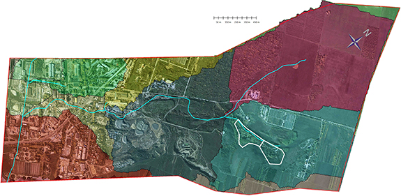
Figure 6. Catchments and potential surface water streams paths around the disposal site. The watershed areas for the topography are shaded in different colours. The potential surface stream network is indicated by the cyan paths.
Download figure:
Standard image High-resolution imageThe disposal facility is within a single watershed of area 1.1 × 10⁶ m2 (green shading). Just south of the flow system outlet from this landscape object there is a confluence with the watershed to the northwest, with area 1.5 × 10⁶ m2 (red shading). Candidate areas for the dose calculations would be located just southwest of the site boundary, before the confluence of the two streams or in the southern area (grey). The water balance of the watershed can be conservatively derived from the net precipitation in the red and green areas, assuming that the water table is closest to the surface near to the indicated flow paths. In this case there is no upstream drainage to consider, the land to the northeast (off the map) sloping away to towards the northeast and draining away from the watersheds shown.
When identifying the candidate areas for the dose objects the requirement is to identify locations in the landscape where the highest concentrations of radionuclides mobilised from the disposal facility could occur and then to set potential exposure pathways, as defined in the design scenario. The aim of the identification process is to define areas in the landscape for potential exposure, they need not necessarily correspond to identified land use in the present day landscape in figure 5. The focus is therefore on areas as close to the disposal site boundary as possible, as stipulated in the ISAM methodology. The procedure is as follows:
- (a)Look for potential areas in the landscape, aided by the orthophoto and topographic details in the digital elevation model using the GIS mapping software.
- (b)Candidate areas should be
- 1.Close to the facility boundary so as to avoid undue spatial dilution,
- 2.Close to the main drainage path as identified from analysis of the digital elevation model, since radionuclides leached from the repository will be transported in the flowing surface and groundwater. If wells are considered in the modelled system placing the objects close to the axis of the drainage system means that the concentration in the local near-surface aquifer will not be underestimated,
- 3.Large enough in area to supply the dietary needs of at least a small family group of, say, four adults. This is typically up to 2 × 10⁴–105 m2.
- (c)Account should be taken of the confluence of drainage systems from different watersheds.
Two candidate objects are indicated in figure 7. The first is closest to the site boundary and is situated on land adjacent to the drainage system that runs through the waste site itself and is along the boundary of the drainage system of the western catchment. The second object is identified by an area along the valley floor of the combined drainage stream. The areas of the two objects are, respectively, 2.1 × 10⁴ m2 and 1.8 × 10⁴ m2.
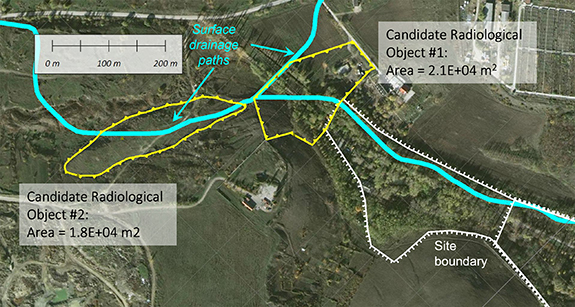
Figure 7. Candidate areas for potential radiological objects. With reference to the orthophoto two areas are identified downslope from the site boundary.
Download figure:
Standard image High-resolution imageAccording to the landuse map (figure 5) the area of Object 1 is currently agricultural land with woodland along the stream location. It is selected as the assessment dose object as the closest location with potential for cultivation to the site boundary. The distance between Object 1 and the disposal facility is about 300 m. Object 2 is classed as non-productive land and natural pasture. For assessment purposes there appears to be no reason why the two areas could not be cultivated, although the land area close to the stream path is relatively steep. According to the orthophoto, the drainage system is not necessarily above ground so a well in the two areas, used for cultivation purposes is the most, realistic approximation. Any surface water stream would be likely to be small and transient.
2.6. Formulation of models
2.6.1. Application of the ISAM approach.
The ISAM RADON example (IAEA 2004b) uses an interaction matrix to express the conceptual model for the site. The interaction matrix is a convenient and compact technique for developing models since it promotes the screening of interactions for specific applications. Furthermore, Kłos and Thorne (2020) have illustrated how interaction matrices can be used to define compartmental mathematical models and we adopt this method here.
Figure 8 is an interaction matrix based on the original ISAM (IAEA 2004a) generic description but processed to include four levels of screening, including those in the IAEA (2004b) documentation. Aggregation and nesting has been used to define the matrix for development into mathematical models for the assessment. We identify the vault and geosphere submodel as distinct from the biosphere submodel. As shown, many interactions are ruled out by generic considerations and others from the description in the ISAM example documentation. Site-specific considerations are used to rule out the interactions as a final stage before translation into mathematical form, thus, we assume that there is no interaction (in terms of radionuclide transport) from the aquifer back to the unsaturated zone and, similarly, that the aquifer is not in contact with the lower soils. Contamination reaches them only via irrigation of the rooting zone soils. Drainage from the system is via the local aquifer. In this form the mathematical models for the vault and geosphere and for the biosphere are defined.
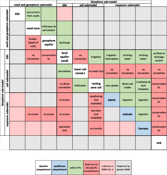
Figure 8. Site-specific IM, describing radionuclide transfers used for model definition. Different submodels are identified for vault and geosphere and for the biosphere. These share a common element—the aquifer/well feature that forms the geosphere–biosphere interface (GBI). Within the biosphere sub-system we distinguish the soils from those elements that are affected by the radiation content of water and soils. Influence from each leading diagonal element on the others is read as the clockwise off-diagonal elements. White shaded elements are treated as dynamic (time varying) compartments and blue as in equilibrium. Details for each model are given in the main text.
Download figure:
Standard image High-resolution imageThe vault/geosphere sub-model describes the release of radionuclides from the waste and transport through saturated media to the site boundary using the ISAM model. Output from the vault/geosphere model is to the Local aquifer defined by the upstream catchment area in figure 6. The interaction matrix indicates that three dynamic compartments are used for the biosphere—the local aquifer (used as a well) the rooting zone soil for crops and the unsaturated soil above the aquifer layer. Xu and Kłos (2021) considered the role played by dynamic soils with equilibrium conditions assumed for the well aquifer, concluding that the dynamics of accumulation of radionuclides in soil was of little significance in the calculation of dose. Here we take the opportunity to add a dynamic aquifer compartment in which accumulation of radionuclides can build up over time with the input from the geosphere aquifer.
The compartmental model equation is used for dynamic compartments:
where the external time-dependent source term to the ith compartment is  Bq yr−1, ingrowth from precursor radionuclide (in the decay chain) is
  Bq yr−1, and transfers to the ith compartment from the other compartments is denoted by
  Bq yr−1, representing the sum of fractional transfers from the other (
 ) compartments. Losses are by radioactive decay
  Bq yr−1, and the sum of all transfers to the other compartments including the sink compartment,
  Bq yr−1. The elements
  of the transfer matrix can be linked to the off-diagonal elements of the interaction matrix (Kłos and Thorne 2020).
2.6.2. Vault and geosphere submodel—scenario SCE1.
Release of radionuclides from the waste is driven by the infiltration of net precipitation through the vault cover, with subsequent percolation to the unsaturated zone and geosphere aquifer. The concentration of radionuclides in the aquifer is constrained by the dimensions of the vault system and the flowpath to the site boundary where mixing with the wider aquifer in the watershed is assumed to take place.
Compartment modelling is an approximation since it is a discretisation of a continuous transport process. Increasing the number of compartments increases accuracy but at the cost of model run-time and model complexity. Based on the guidance of Kirchner (1998) and Xu et al (2007) the optimal number of compartments can be determined. As shown in figure 9, the waste form is modelled by a single compartment, the unsaturated zone by three and the aquifer downstream from the disposal facility by five compartments.
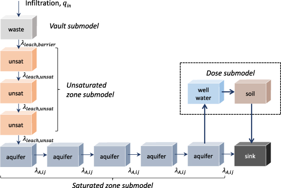
Figure 9. Compartmental model of radionuclide transport (scenario SCE1) disaggregated from the interaction matrix in figure 8. Grey is the vault model with the orange compartments the unsaturated zone, with blue the geosphere aquifer. The biosphere submodel is shown as distinct from the geosphere submodel. Details of the vault/geosphere submodel are given by Xu and Kłos (2021).
Download figure:
Standard image High-resolution image2.6.3. Biosphere submodels and geosphere–biosphere interface (GBI)—scenario SCE1.
The compartment structure in the interaction matrix (figure 8) is a disaggregation of the soils/sediments leading diagonal element of the ISAM (IAEA 2004b) interaction matrix. Figure 10 shows the transfer processes in the GBI/soil submodel. The source term to the biosphere model is defined by the radionuclide flux from the vault/geosphere model. This constitutes a time series into the biosphere and the transfer coefficients are defined as shown in figure 10.
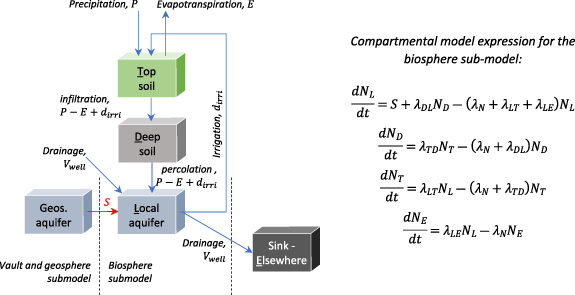
Figure 10. Dynamic compartments in the dose sub-model. The geosphere–biosphere interface is a well in the local aquifer (L) through which the upstream catchment drains to the sink (E). Rooting zone (T) and unsaturated soils (D) are include as described in Xu and Kłos (2021) with inventories denoted by  , for
, for  . Input from the vault/geosphere model,
  , is to the local aquifer.
Download figure:
Standard image High-resolution imageFrom equation (2), the radionuclide inventories in the compartments L, D, T, E vary as shown in figure 10 and the solute mediated transfers from compartment i to compartment j are given by Kłos and Thorne (2020) as

where the water flux is  , the compartment saturation is
  , the porosity
  , the density
  . The thickness of the compartment is
  and plan area
  , giving an overall compartment volume
  .
.  is the radionuclide decay. The retardation factor for the radionuclide in the compartment is

where  is the Kd-value for the radionuclides in the ith compartment and
  the grain density of the solid material in the compartment.
The area of the soil layer,  , corresponds to that of the biosphere object defined in figure 7 and the annual precipitation (
 ), evapotranspiration (
 ) and irrigation (
 ) amounts are defined by the site context, so that water conservation gives water fluxes in the soil as

The water flux from well to topsoil is the irrigation demand,

The justification of a suitable dilution parameter for wells—here  —is a well-known problem in site-generic studies or in cases with limited site characterisation. The well dilution is not well defined in the ISAM documentation. A value of 8300 m3 yr−1 is used as the flow rate in the well but the site context differs somewhat from that considered here. Similarly, the volume of the well compartment is not precisely defined in the ISAM examples. Here, however, we are able to bound these key parameters from the site-description. For the volumetric flow in the well there are two bounding cases.
2.6.3.1. Minimum dilution in local aquifer.
Flow in the well is defined as the total abstraction for domestic and agricultural purposes within the biosphere object. With object area 2.1 × 10⁴ m2 and irrigation demand 0.3 m yr−1 the irrigation requirement is 6.3 × 10³ m3 yr−1. This dominates the water usage for the assumed exposed group, drinking water consumption for four adults assumed is around 3 m3 yr−1 and livestock consume around 22 m3 yr−1 (data from Xu and Kłos 2021). The minimum dilution case therefore assumes  = 6.3 × 10³ m3 yr−1, similar to the ISAM example.
2.6.3.2. Maximum dilution in local aquifer.
Water in the local groundwater flow system is that captured by the upstream catchment. The maximum dilution case uses the total net precipitation,  , taking
  = 1.1 × 10⁶ m3 and precipitation and evapotranspiration 0.573 and 0.460 m yr−1, respectively, the maximum dilution case therefore assumes
  = 1.24 × 10⁵ m3 yr−1.
These two values express the limits of the dilution parameter. The maximum case assumes all of the upstream inflow dilutes the input from the vault/geosphere model which is consistent with the single compartment approximation for the well aquifer though it can be understood as unlikely. The minimum dilution case is similarly an extreme but it is clear that the true dilution lies between these limits and a uniform distribution is suitable for sensitivity and uncertainty analyses. There is no preferred value without a more detailed model for groundwater flow in the local area but results are suitable for initial assessment purposes since the range is linked directly to local conditions via analysis of the topography (GIS) and understanding of the local geology (Anton 2017, Dimo and Mosoi 2018). For the deterministic calculations we use the 8300 m3 yr−1 value from the ISAM example as a reference case.
2.6.3.3. Maximum well compartment volume.
The volume of the 'well compartment' can be bounded by assuming that the total volume of the well is, as an upper limit, the volume of the compartment defined by the area of the biosphere dose object (figure 7) and the thickness of the aquifer layer (20 m from Dimo and Mosoi 2018). So  = 4.2 × 10⁵ m3. This is again consistent with the assumptions for single compartment approximation.
2.6.3.4. Minimum well compartment volume.
In a review of hydraulics of water wells Houben (2015) gives that the radius of the zone affected by an abstraction borehole is about 1.5 times the depth of the aquifer, which might be used to estimate the minimum size of the well compartment. The minimum well volume is then  = 5.6 × 10⁴ m3.
These limits are, again, suitable for the scoping purposes here. Further site characterisation could be carried out to obtain better definition but for early stage assessments the ranges and the method of determining them is appropriate to the assessment context.
2.6.3.5. Equilibrium solution.
The system of equations for the biosphere submodel can be solved for the equilibrium conditions so that all inventories can be linked back to the radionuclide release flux from the vault/geosphere submodel. Results from Xu and Kłos (2021) show that the timescales associated with equilibrium in the topsoil and deep soil compartments have little influence on the timing and magnitude of the calculated doses when equilibrium conditions in the well compartment are also adopted. With the dynamic aquifer model here a further comparison can be made to assess the effect on dose of full dynamics in the biosphere system.
2.6.3.6. Exposure submodel.
Doses to the human exposed group are expressed as a linear sum over the exposure all pathways arising from water and soil via the different exposure routes,

The pathways include those identified in the column for humans in figure 8, namely ingestion, inhalation and external irradiation. The conversion factors  ,
,  depend on the description of the exposure route r and the intake (exposure) rates,
  ,
,  , combine different processes. For example, consumption of meat from domesticated animals requires the transfer factors from the intake of radionuclides in the animal in fodder as well as the consumption of water. The intake of radionuclides in crops depends on the uptake of radionuclides in the soil via the roots as well as the intercepted radionuclides that originate in well water used for irrigation. In the equilibrium biosphere, equation (7) reduces to a sum over all exposure routes only from the source term to the biosphere submodel in figure 10.
2.6.4. Models for the alternative and human intrusion scenarios—SCE6, SCE7.
Analytical models are used for the two human intrusion scenarios selected, namely the on-site residence scenario SCE6 and the road construction scenario SCE7, taken from the ISAM RADON test case. Two further alternative scenarios are included: the flooding scenario and the landslides scenario. The model used for the flooding scenario is the so-called bathtubbing model adapted from the ISAM test cases, employing an analytical expression describing radionuclides in overflowing leachate. For landslides we assume that results of the on-site residence scenario SCE6 are appropriate. Xu and Kłos (2019, 2021) give details.
3. Results
3.1. Model implementation and data sources
The models described in the previous section were implemented for deterministic and probabilistic analyses using Ecolego 6.5 (Ecolego 2018). This section gives results from the various scenarios and calculation cases. All data used in simulations can be found in Xu and Kłos (2021) with the exception of data for the dynamic soil and aquifer submodel which are summarised in table 2. We have made as much use of site-specific information as possible in deriving parameter values used in the assessment. The rest of the data used are adapted from ISAM reports (IAEA 2004a, 2004b) and IAEA Technical Document 1380 (IAEA 2003b).
Table 2. Parameters for the dynamic compartments in the biosphere/aquifer submodel.
| Parameter | Symbol | Unit | Value | Distribution | Source |
|---|---|---|---|---|---|
| Precipitation |

| m yr−1 | 0.573 | — | Anton (2017) |
| Evapotranspiration |

| m yr−1 | 0.46 | — | Anton (2017) |
| Area of biosphere object |

| m2 | 2.10 × 10⁴ | — | Section 2.5 |
| Area of upstream catchment |

| m2 | 1.10 × 10⁶ | — | Section 2.5 |
| Irrigation demand |

| m yr−1 | 0.3 | Uniform: min 0.025, max 0.5 | Xu and Kłos (2021) |
| Well capacity |

| m3 yr−1 | 8.3 × 10³ | Uniform: min 6.3 × 103 max 1.24 × 105 | ISAM (IAEA 2004b) and section 2.6.3 |
| Volume of the well compartment |

| m3 | 5.65 × 10⁴ | Uniform: min 5.65 × 104 max 1.3 × 105 | Section 2.6.3 |
3.2. Results from the design scenario SCE1
3.2.1. Limiting values for dose—deterministic model.
The limits on the aquifer and well parameters can be used to define the range of doses in the biosphere dose object, the results are plotted in figure 11 showing the four combinations in table 2 for the flow and volume parameters and the ISAM reference flow rate as well as the equilibrium dose result for accumulations of radionuclides in the biosphere submodel.

Figure 11. Range of deterministic results due to the limiting values for aquifer flow rate and well volume during the 100 kyear assessment period. For reference the ISAM dilution is used with the minimum well volume and a case with the equilibrium solution for the biosphere compartments are shown. The radionuclides contributing to dose at the times of the four maxima are indicated.
Download figure:
Standard image High-resolution imageAs there is no site-specific preferred value for either aquifer dilution or well volume, the actual doses can be expected to lie somewhere between these cases. There are three distinct peaks—for 36Cl around 10 years, 14C (1 kyear) and 239Pu (20 kyear), as well as an increasing dose, towards the end of the simulation period, arising from 210Po, the short lived progeny of the 226Ra initially present in the repository. The ratio of maximum dose to minimum is around a factor of 20 in each case and this is close to the ratio of the limits of the overall dilution factor. The size of the well compartment has less of an influence but this has the most impact in the low dilution cases where the ratio of volumes (=2.3) corresponds to the reduction of dose in the two low dilution cases. As may be anticipated, the ISAM dilution gives results close to the upper limit since it is close to the minimum determined by site-specific considerations.
The dynamic aquifer plays a role in determining the timing of dose. This is most apparent in the low dilution cases where the larger the aquifer compartment volume, the longer the time to equilibrium required. Although the effect is small it is clear that the assumption of equilibrium conditions in the aquifer compartment as well as the soils (see Xu and Kłos 2019) would give slightly earlier dose peaks for the less strongly sorbing 36Cl and 14C and the higher sorbing 239Pu and 226Ra peaks would occur much earlier. This indicates that understanding the groundwater system is of more importance than the soil system in this case whereby the soils become contaminated via the use of well water.
These deterministic results show that the maximum doses for the unremediated facility could approach the 0.3 mSv yr−1 dose limit specified by the IAEA but this would be after several thousand years (14C) and far in the future for 239Pu and the 226Ra chain (after 10 kyear). In each of these cases the dilution is at the lower extreme of the site-specific values. This prompts further consideration of the model. The behaviour of 14C in the biosphere means that it is not well represented by the kind of model described here and more detailed 14C-specifc models are required for more reliable dose estimation. The models for 239Pu and the 226Ra chain are appropriate for the purposes but the timescale for the peak doses to arise is over 10 kyear and, on such a timescale, major change to the biosphere system would be likely to take place, not least there might be erosion and redistribution of contaminated material in the vault-aquifer-biosphere system. Nevertheless the results from the SCE1 deterministic case suggest that remedial action to safeguard the site should be considered.
3.2.2. Probabilistic calculations and sensitivity analysis.
Avila et al (2010) categorise parameters used in simulations as (a) time-independent parameters considered to be certain, (b) time-independent parameters with uncertain values, and (c) time-dependent parameters. Parameters in the first category are those representing habits and properties of the exposed individuals, such as inhalation rates, water ingestion rates food ingestion rates and dose coefficients. Other time-independent parameters fall into the second category and the effect of their uncertainty on the calculated total dose is studied by performing probabilistic simulations. These parameters are distribution coefficients and parameters used in determining transfer factors illustrated in the conceptual model in figure 8.
Six parameters connected with the transfer rates were studied using 3000 sample sets generated using Latin hypercube sampling:
- volume of the well compartment (uniform: 5.65 × 10⁴–1.3 × 10⁵ m3),
- well capacity (uniform: 6.3 × 10³–1.24 × 10⁵ m3 yr−1),
- hydraulic conductivity in the geosphere aquifer (uniform: 0.2–0.5 m d−1, best estimate 0.35 m d−1),
- effective porosity in the geosphere aquifer (uniform: 0.2–0.4, best estimate 0.35),
- irrigation rate (uniform: 0.25–0.4 m yr−1, best estimate 0.3 m yr−1),
- Kd values for radionuclides in the clay, saturated layers and soils. The values from IAEA (2003b) are here used as the geometric mean and we assume—for purposes of sensitivity analysis—the geometric standard deviation is 2.0 for all elements and for all media.
Uncertainty analysis results are plotted in figure 12, showing that the range from the 2.5th to the 97.5th percentile encompasses the deterministic results, thereby indicating that the uncertainty in vault and geosphere parameters contributes significantly to overall uncertainty. The probabilistic results spread out the time dependence of calculated doses by virtue of the retardation effects of the sampled Kd values. Overall, however, the peak doses in this probabilistic uncertainty analysis are similar to those as determined by the range of values determined by the uncertainty in the aquifer/well characteristics. The arithmetic mean and median doses imply peak doses around 5 × 10⁻² mSv year−1. It should be remembered, however, that the distribution assumed for the well dilution parameter is uniform between the limits defined from the site-specific conditions and, as such, the range of results is a more reliable indicator of the radiological hazard. This is suitable for scoping studies but the central values in the probabilistic analysis are heavily influenced here by the uniform distribution and there is no preferred value for well dilution on the basis of the information available.
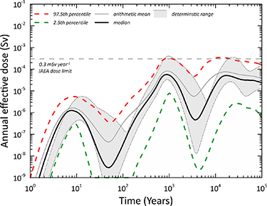
Figure 12. Time series of different statistics of the total doses from probabilistic simulations, in which the arithmetic mean, median, 2.5th and 97.5th percentiles are shown. The range from the deterministic calculations is also plotted giving an indication of the variability from parameters other than the well characterisation.
Download figure:
Standard image High-resolution imageA probabilistic sensitivity analysis was carried out using standardised rank regression coefficients (SRRCs). The higher the absolute SRRC for an input parameter, the greater the effect on the output. A positive SRRC value indicates that input and output move in the same direction, whereas a negative SRRC value shows that they move in the opposite sense. Results for the three main peaks in figure 12 are shown in table 3.
Table 3. Result for standardised rank correlation coefficients (SRRC >≈ 0.1) in the probabilistic analysis at 10 year, 1 kyear and 20 kyear.
| 10 years (36Cl) | 1 kyear (14C) | 20 kyear (239Pu) | |||
|---|---|---|---|---|---|
| Parameter | SRRC | Parameter | SRRC | Parameter | SRRC |
Well dilution, 
| −0.79 | Well dilution, 
| −0.63 | Saturated aquifer Kd, 239Pu | −0.71 |
| Soil Kd, 36Cl | 0.28 | Soil Kd, 14C | 0.58 | Darcy velocity in geosphere aquifer | 0.42 |
| Darcy velocity in geosphere aquifer | 0.17 | Saturated zone Kd, 14C | −0.18 | Unsaturated zone Kd, 239Pu | −0.29 |
Irrigation demand, 
| 0.14 | Irrigation demand, 
| 0.09 | Saturated zone Kd, 226Ra | −0.21 |
| Well volume | −0.13 | ||||
Well dilution, 
| −0.13 | ||||
Doses at earlier times (up to 1 kyear) come from the more weakly sorbing radionuclides in the vaults and, as might be expected, the well dilution has the greatest influence, acting to flush any radionuclides reaching the aquifer rapidly out of the biosphere dose object. Retention in the rooting zone soil is positively correlated for the 36Cl and 14C peaks and irrigation demand is seen to have a relatively small influence on dose. Flow in the geosphere aquifer has the effect of transporting 36Cl to the biosphere object and retention of 14C in the saturated zone of the geosphere flow path is negatively correlated.
The later peak is more complex, since retardation in the geosphere aquifer dominates with a high negative correlation, acting to delay the arrival of 239Pu into the biosphere object, as does the Kd in the unsaturated zone. These contrast with the positive correlation of the aquifer's Darcy velocity. The saturated zone Kd for 226Ra is flagged as influencing the dose at this later peak via its effect on the progeny, 210Po. For the more strongly sorbing radionuclides that appear at this peak, the well characteristics are of lesser importance.
The uncertainties in the SCE1 scenario are emphasised in the analysis. 36Cl could possibly be detectable at boundary of the site in the present day but doses would be low as the biosphere object is not currently cultivated. The inherent uncertainties in the dose assessment for 14C means that the results here are indicative of the potential for 14C to be of interest but at around 1 kyear after present. Action by the local authorities may be anticipated well before this could become an issue, as is also the case for 239Pu and 226Ra. Results from the SCE1 scenario therefore suggest that remediation of the site should be considered and this feeds into the assessment of the other exposure scenarios.
3.3. Results from the human intrusion scenarios (scenarios SCE6 and SCE7)
The on-site residence scenario (SCE6) assumes that the engineered barriers of the disposal facility as well as the waste are totally degraded. The exposed residents in this scenario are assumed to live in a house built directly on top of the facility. Due to this distribution of waste material, the soil around the house is expected to be contaminated at a level equal to the specific activity of the waste divided by a dilution factor. Residents grow vegetables in the garden for their own consumption.
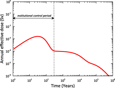
Figure 13 shows the results for the total dose for this scenario and main radionuclides contributed to the doses. The maximum total dose is about 130 mSv, after around 6 kyear. The results show that human intrusion activities after the control period can lead to radiological exposure significantly above the level of 1 mSv for up to 100 000 years. The main radionuclides contributing to the doses are 239Pu and its progeny nuclides, as well as 226Ra, 210Pb and 210Po.

Figure 13. Total annual effective dose for the on-site residence scenario, showing results of the main radionuclides contributing to dose. Institutional control is assumed to be maintained up to 300 years after the start of the simulation.
Download figure:
Standard image High-resolution imageThe road construction scenario (SCE7) anticipates that the engineered barriers of the disposal facility as well as the waste are totally degraded. Road construction is assumed to be directly across the disposal facility. The situation is considered as very unlikely to occur but, were it to do so, potentially an important radiological impact could arise. The maximum total dose is about 13 mSv, with doses dominated by 239Pu at times up to 100 kyear.
3.4. Results from the alternative scenarios
From section 2.3 two alternative scenarios were selected to assess the significance of potential deviations from the reference evolution for the long-term safety of the disposal facility: the flooding and landslides scenarios. The frequency of flooding occurring is described by equation (1) and the consequence of the flooding scenario is described by the bathtubbing case. Thus, the effective risk or the effective annual doses for this event occurring before that time of evaluation should be considered and may be expressed for discrete events as (Bergström et al 2008):
where  is the effective annual dose at time T (Sv),
  is the frequency of the occurrence at time t (-) (equation (1)),
  is the annual dose at time T associated with any event at time t (Sv), which is calculated by the bathtubbing model. Figure 14 shows the calculated effective annual dose due to flooding event with the frequency considered during the whole assessment period. The maximum total annual effective dose is 1.56 mSv occurring at around 30 years post closure. However, the calculated dose is based on the model that describes radionuclides in overflowing leachate with the on-site residence exposure pathways. During this time, the site is expected to remain under institutional control and measures would be expected to be taken were such flooding events to occur. As noted, the result of the on-site residence scenario can cover the landslides scenario, therefore, no separate calculation was performed.
Figure 14. Total effective annual dose for releases from the disposal facility due to the flooding event of the alternative scenario. For this simulation, the possibility of flooding during the institutional control period of 300 year is included.
Download figure:
Standard image High-resolution image
3.5. Results of the assessment for non-human biota
The potential effects on non-human biota from exposure to released radionuclides were also assessed as part of this assessment. The maximum values of the radionuclide concentrations in soil over simulation times were obtained. These values were then divided by the corresponding EMCLs, which have been derived in the ERICA project 6 . The resulting values are the so-called risk quotients (RQs), following the graded approach proposed in ERICA. According to this screening method, if the RQs are below one, it can be understood that risks to biota are insignificant and no further assessments are required. If the RQ are above one, then more detailed assessments should be undertaken.
The soil concentrations obtained from the deterministic calculations for the well case were found to give EMCL values below are 1 except for 14C with a RQ value of 5. This indicates that a more detailed assessment would be required. As noted above, however, the model for radionuclide transport and accumulation in the biosphere (as used in the ISAM examples) is not ideally suited to 14C. Further assessment for non-human biota may be considered in connection with future developments of an alternative model for 14C dose assessment. Furthermore, this analysis does not take into account conditions within the facility boundary.
3.6. Summary of results for human exposure
As a summary, the calculated peak doses and time at which the peak is observed from six human exposure scenarios/calculation cases are shown in table 4.
Table 4. Peak annual dose and time after the closure at which the peak is observed from six scenarios/calculation cases.
| Scenarios | Descriptions | Peak dose (mSv) | Years | IAEA (2011) dose criterion (mSv yr−1) | |
|---|---|---|---|---|---|
| Design scenario | SCE1 | Well biosphere (deterministic) | 0.03–0.4 | 1 000 | 0.3 |
| Arithmetic mean (probabilistic) | 0.08 | 1 000 | |||
| 97.5th percentile | 0.35 | 11 000 | |||
| 2.5th percentile | 0.008 | 1 000 | |||
| Alternative scenarios | Flooding | 1.6 | 30 | 0.3 | |
| Landslides a | 130. | — | 0.3 | ||
| Human intrusion scenarios | SCE6 | On-site residence | 130. | 300 | 20. |
| SCE7 | Road construction | 13. | 300 | 20. | |
a Calculated dose not taking into account the frequency of occurrence.
4. Discussion
Following the ISAM methodology (IAEA 2004a, 2004b) helps to provide assurance that the assessment has effectively addressed all potentially relevant FEPs and taken account of the ways in which combinations of these FEPs might produce qualitatively different outcomes. The systematic approach also provides the framework for demonstrating how uncertainties associated with the future evolution of the disposal system have been addressed and assimilated into the safety case.
Following the BIOMASS methodology and including a site-specific digital elevation model allowed the relevant biosphere object and associated catchment areas to be identified using GIS tools, so that local characteristics could be incorporated into the generic ISAM model framework. The methods for model definition discussed in the MODARIA II update of the BIOMASS methodology (IAEA 2020, Kłos and Thorne 2020) have been used to audit the model description from IAEA (2004b) so as to justify the model FEPs implemented.
The issue of dilution in the aquifer is a well-known problem, particularly for generic assessments such as the ISAM example. Site characterisation involving hydrological modelling can produce detailed descriptions of local-scale hydrology in radiological assessments. The method used here is somewhat simpler and is suitable for scoping studies such as this. Using site-descriptive modelling we demonstrate a simple method for bounding well capacity, and thereby the activity concentration in well water, using a straightforward understanding of water balance in the local watershed area associated with the biosphere object. Minimum dilution is conservatively determined by the irrigation demand for the object. Site-specific constraints are used to determine the upper bound for the well volume and a simple expression is used to provide the lower bound, based on the depth of the aquifer that underlies the biosphere object.
In this assessment the well scenario included a fully dynamic soil and aquifer submodel for the biosphere component of the dose assessment model. Although the dynamic soil compartments are close to equilibrium with the aquifer the timescale for equilibrium conditions in the aquifer compartment is long enough that the equilibrium model for the biosphere/aquifer gives noticeably different results (figure 11). Moreover, to determine the equilibrium expressions (relating biosphere concentration back to the discharge from the geosphere aquifer) requires a full description of the biosphere subsystem (figure 10). Adding the dynamic details to the compartment model solver adds few overheads to the overall solution of equation (2) for the whole model and so is the preferred choice for the dose assessment model.
It should also be noted that the dynamics of the soil compartments relate to the time for the soil compartments to reach dynamic equilibrium. As modelled here irrigation is the only route by which activity from the well reaches the rooting soils with continuous irrigation for the entire assessment period of 100 kyear. This can be seen to be a conservative assumption since cultivation of the same area of land over this period is rather unlikely. Direct irrigation interception by cultivated crops is included in the model and Xu and Kłos (2021) note that this gives doses around 5% of the values when long-term irrigation is included.
Uncertainty and sensitivity analyses indicate that the most sensitive parameter around the time of peak dose is the well capacity,  , which is negatively correlated to the total dose and is directly related to groundwater dilution. The other dominant parameters (at the times chosen for analysis) are the soil Kds (in the unsaturated geosphere and the rooting zone soil) for 36Cl (10 year), 14C (∼1 kyear) and 239Pu (20 kyear). The Darcy velocity in the downstream geosphere from the vaults is also a key feature for the more strongly sorbing radionuclides in the vaults (239Pu and 226Ra). The well parameter dilution is of lesser importance for the high Kd radionuclides but the well volume is seen to have a weak influence on peak dose at the later times.
The design scenario (SCE1) is a necessary part of the assessment since it deals with potential exposures beyond the facility boundary where no institutional control is assumed. The modelling indicates that the 0.3 mSv yr−1 dose criterion (IAEA 2011) could be exceeded in the SCE1 cases in the case of low well dilution but it should be remembered that the low dilution limit is based on a very small flow in the aquifer, equivalent to the irrigation demand. There are good reasons to see this as overly conservative but the method here provides bounds for the assessment. The 97.5th percentile in the probabilistic uncertainty analysis is similar in magnitude to the limit used in the deterministic cases but this is linked closely to the assumed uniform distribution of flow rate between the upper and lower bounds. The probabilistic calculations for SCE1 are most useful for sensitivity analysis as these indicate where resources would be directed should it be required to perform more detailed site characterisation, for the better understanding of the local hydrology for example. Without long-term accumulation in soils the doses should it be at least an order of magnitude lower. Attention then turns to the other scenarios identified for analysis.
The alternative scenarios—flooding and landslides—give significantly higher doses, flooding being mitigated by the probability of flooding as a function of time. Results for the human intrusion scenarios are also relatively high although the IAEA (2011) dose criteria differ between the scenarios considered. Results for the activity retained in the repository structures provide input to the regulatory decisions that need to be taken in respect of the radiation options for the facility.
5. Conclusions
We have adopted ISAM and BIOMASS methodologies to perform the risk assessment for the RADON-type of near-surface disposal facility near Chişinău, illustrating practicality of applying these methodologies to site-specific dose assessment problems. By using GIS techniques based on a site-specific digital elevation model, a method for identifying relevant biosphere objects so as to customise the generic model from ISAM to a site-specific model is demonstrated.
From site-specific understanding we have demonstrated a simple method for bounding well capacity, and thereby the activity concentration in well water, using a straightforward understanding of water balance in the local watershed area associated with the biosphere object. In this way the maximum dilution of contaminants released from the disposal facility in aquifer can be estimated. Site-specific constraints are also used to determine the upper bound for the well volume and a simple expression is adopted to provide the lower bound, also based on the depth of the aquifer that underlies the biosphere object.
With conservative assumptions, estimated doses from the calculation cases of the design scenario are close to the IAEA's dose criterion but these are determined by the most pessimistic assumptions concerning well dilution. However, estimated doses for the on-site residence scenario after institutional control are higher than IAEA's criterion. The results show that human intrusion activities after the institutional control period can lead to radiological exposure above the level of 1 mSv yr−1 for up to 100 kyear. Long lived 239Pu dominates doses for on-site residence. Of course, the suitability of the very conservative assumptions used in the modelling of the on-site residence scenarios can be debated. Nevertheless, remedial measures should be considered for the waste in the repository in its current state. The disposal facility is located upstream of Chişinău, which might, in hindsight, not have been an optimal choice as a site for a radioactive waste disposal.
This assessment has had the primary function of assessing potential radiological impacts thereby identifying where better local information might reduce conservatism and lead to a more realistic expression of the assessment of radiological impact.
The results from the assessment here indicate that 14C is a significant radionuclide in the inventory and the calculated doses have used the form set out in the ISAM model description. This treats 14C using a standard transport and dose model that is common to other radionuclides. It is known, however, that 14C shows behaviour that is not well represented by such models since the soil-atmosphere-plant continuum is not directly considered. Future developments might consider the possibility of alternate model for 14C dose assessment. Nevertheless the results here may be considered suitable for a first-look assessment to scope the problem.
Acknowledgments
This study has been financed by the Swedish Radiation Safety Authority (SSM). We would like to thank the anonymous reviewers for their time and effort improving the quality of our manuscript.
Footnotes
- 5
Copyright © 2019 Blue Marble Geographics.
- 6
Environmental Risk from Ionising Contaminants: Assessment and Management.
EC-EURATOM 6 Framework Programme (2002–2006). Project Contract FI6R-CT-2004-508 847.