

Abstract
The linear response is a perturbation theory establishing the relationship between given physical variable and the external field inducing this variable. A well-known example of the linear response theory in magnetism is the susceptibility relating the magnetization with the magnetic field. In 1987, Liechtenstein et al came up with the idea to formulate the problem of interatomic exchange interactions, which would describe the energy change caused by the infinitesimal rotations of spins, in terms of this susceptibility. The formulation appears to be very generic and, for isotropic systems, expresses the energy change in the form of the Heisenberg model, irrespectively on which microscopic mechanism stands behind the interaction parameters. Moreover, this approach establishes the relationship between the exchange interactions and the electronic structure obtained, for instance, in the first-principles calculations based on the density functional theory. The purpose of this review is to elaborate basic ideas of the linear response theories for the exchange interactions as well as more recent developments. The special attention is paid to the approximations underlying the original method of Liechtenstein et al in comparison with its more recent and more rigorous extensions, the roles of the on-site Coulomb interactions and the ligand states, and calculations of antisymmetric Dzyaloshinskii–Moriya interactions, which can be performed alongside with the isotropic exchange, within one computational scheme. The abilities of the linear response theories as well as many theoretical nuances, which may arise in the analysis of interatomic exchange interactions, are illustrated on magnetic van der Walls materials CrX3 ( Cl, I), half-metallic ferromagnet CrO2, ferromagnetic Weyl semimetal Co3Sn2S2, and orthorhombic manganites AMnO3 (
 La, Ho), known for the peculiar interplay of the lattice distortion, spin, and orbital ordering.
Export citation and abstract BibTeX RIS

Original content from this work may be used under the terms of the Creative Commons Attribution 4.0 license. Any further distribution of this work must maintain attribution to the author(s) and the title of the work, journal citation and DOI.
1. Introduction
On many occasions our image of magnetism rests on the picture interacting spins (
e
i
and
e
j
) attached to the atomic sites (i and j). If the system is isotropic, such interactions have a form of the scalar products  [1–5]. The interactions are ferromagnetic (FM) if they force
  and antiferromagnetic (AFM) if
  . If i and j are no longer connected by the spacial inversion, the spins tend to align neither ferromagnetically nor antiferromagnetically.
1
The corresponding interaction, which is called Dzyaloshinskii–Moriya (DM) interaction, is given by the cross product
. If i and j are no longer connected by the spacial inversion, the spins tend to align neither ferromagnetically nor antiferromagnetically.
1
The corresponding interaction, which is called Dzyaloshinskii–Moriya (DM) interaction, is given by the cross product ![$[\boldsymbol{e}_{i} \times \boldsymbol{e}_{j}]$](https://content.cld.iop.org/journals/0953-8984/36/22/223001/revision2/cmad215aieqn6.gif) and driven by the relativistic spin–orbit (SO) coupling [6, 7]. Thus, it is always nice to have a transparent toy model, which would explain that certain material has a particular magnetic structure because some interactions are strong or weak, FM or AFM, etc. The experimental inelastic neutron scattering data are typically fitted to extract parameters of such physically meaningful model. In theory, the spin model can be constructed by averaging the energies of interatomic interactions over non-magnetic degrees of freedom [1–5, 7]. In this article we will explain how the interatomic exchange interactions can be generally derived starting from the electronic structure obtained in the first-principles calculations.
and driven by the relativistic spin–orbit (SO) coupling [6, 7]. Thus, it is always nice to have a transparent toy model, which would explain that certain material has a particular magnetic structure because some interactions are strong or weak, FM or AFM, etc. The experimental inelastic neutron scattering data are typically fitted to extract parameters of such physically meaningful model. In theory, the spin model can be constructed by averaging the energies of interatomic interactions over non-magnetic degrees of freedom [1–5, 7]. In this article we will explain how the interatomic exchange interactions can be generally derived starting from the electronic structure obtained in the first-principles calculations.
Let us consider the simplest possible spin model with the energy

where Jij
is the isotropic exchange,  is DM vector, and the spin moments
e
i
are normalized to the unity:
is DM vector, and the spin moments
e
i
are normalized to the unity:  . Although we will be primarily interested in the behavior of isotropic interactions, it appears to be possible to consider Jij
in the combination with
d
ij
within one computational scheme. The reason will become clear in a moment. Our goal is to find parameters of this model using the information about the electronic structure. Of course, the model (1) is an approximation as there is no reason why the energy of a general magnetic system should have such a simple form and be described exclusively by the bilinear interactions. There are only few microscopic mechanisms, which are consistent with the form of equation (1). These are the direct Heisenberg exchange [1], Anderson's superexchange [2], and long-range exchange interactions by Ruderman, Kittel, Kasuya, and Yosida (RKKY) [3–5, 8, 9]. In the first example, this is the property of exchange energy, related to the antisymmetry of fermionic wave functions. In the last two examples, this is the consequence of the 2nd order perturbation theory with respect to, respectively, transfer integrals and intra-atomic exchange interactions, that couples localized core spins to the outer conduction electrons.
. Although we will be primarily interested in the behavior of isotropic interactions, it appears to be possible to consider Jij
in the combination with
d
ij
within one computational scheme. The reason will become clear in a moment. Our goal is to find parameters of this model using the information about the electronic structure. Of course, the model (1) is an approximation as there is no reason why the energy of a general magnetic system should have such a simple form and be described exclusively by the bilinear interactions. There are only few microscopic mechanisms, which are consistent with the form of equation (1). These are the direct Heisenberg exchange [1], Anderson's superexchange [2], and long-range exchange interactions by Ruderman, Kittel, Kasuya, and Yosida (RKKY) [3–5, 8, 9]. In the first example, this is the property of exchange energy, related to the antisymmetry of fermionic wave functions. In the last two examples, this is the consequence of the 2nd order perturbation theory with respect to, respectively, transfer integrals and intra-atomic exchange interactions, that couples localized core spins to the outer conduction electrons.
Nevertheless, there is one more, very special case, where the magnetic energy can be also described by equation (1). These are the infinitesimal rotations of spins near the equilibrium, as was realized by Liechtenstein et al [10, 11]. Indeed, considering rotations  near the ground state
  (
( being the position of the site
  ,
,  being the spin-spiral propagation vector), one can evaluate the energy change (per one unit cell) caused by interactions between the transversal (xy) components of spins. For the model (1), this energy change is given by

where  is the Fourier image of Xij
. Then, the basic idea is to extract the same energy change from the electronic structure calculations, typically within spin-density functional theory (SDFT) [12–14], and map it on equation (2). This should give us the parameters of exchange interactions
is the Fourier image of Xij
. Then, the basic idea is to extract the same energy change from the electronic structure calculations, typically within spin-density functional theory (SDFT) [12–14], and map it on equation (2). This should give us the parameters of exchange interactions  and
and  (or Jij
and
(or Jij
and  after the Fourier transform to the real space). Since the rotations of
e
i
are chosen in the form of the conical spin spiral (which is compatible with the DM interactions), Jij
can be considered in the combination with
after the Fourier transform to the real space). Since the rotations of
e
i
are chosen in the form of the conical spin spiral (which is compatible with the DM interactions), Jij
can be considered in the combination with  in the one computational scheme, where the energy change is uniquely specified by
q
[15]. Basically, this is a perturbation theory, which can be formulated in terms of the response function (or the susceptibility).
in the one computational scheme, where the energy change is uniquely specified by
q
[15]. Basically, this is a perturbation theory, which can be formulated in terms of the response function (or the susceptibility).
One of the most attractive points of the infinitesimal rotations of spins is that the bilinear form of equation (1) remains valid irrespectively on which microscopic mechanism stands behind the interaction parameters. It can be the superexchange [2], RKKY [3–5], double exchange [16] or any other mechanism, provided that the rotations are small. Even biquadratic exchange [17] for small θ can be reformulated in the bilinear form (1). Without SO coupling, the energy change caused by the infinitesimal rotations of spins can be always described by the Heisenberg model and in this sense the method is very universal.
Another important point of the work of Liechtenstein et al [11] is that they have proposed a practical scheme for calculating the exchange parameters and proved for these purposes the magnetic force theorem [18–20], which justifies the use of the single-particle energies, obtained from the Kohn–Sham (KS) equations in SDFT [13, 14], for evaluating the energy change caused by the infinitesimal rotations of spins. The theorem greatly simplifies the calculations and improves the numerical accuracy.
The basic variable of SDFT is the magnetization density  . In the ground state,
  is controlled by the exchange–correlation (xc) field
  . Therefore, instead of rotating
  , Liechtenstein et al [11] have proposed to rotate
  , assuming that
  will automatically rotate by the same angle. This leads to the commonly used expression for Jij
:
will automatically rotate by the same angle. This leads to the commonly used expression for Jij
:

which is nothing but the 2nd order perturbation theory for the single-particle energy, formulated in terms of the single-particle Green's functions  with the spins
 or
or  (
( being the Fermi energy,
  stands for the trace over orbital indices, and
  denotes the imaginary part). Although this result was anticipated by the previous works on the RKKY interactions [5, 8], the exchange interactions in the paramagnetic medium [21, 22], as well as general theories of the itinerant magnetism [23, 24], the expression (3) can be relatively easily combined with the first-principles electronic structure calculations for the ground state, in the framework of SDFT or its refinements. Today, it is known for almost 40 years and was successfully applied for the analysis of interatomic magnetic interactions in various substances [25–32].
Nevertheless, there are also open questions. Particularly, several authors have raised doubts that the true energy change caused by the infinitesimal rotations of spins can be described by rotating only  and suggested that it should include the additional contribution steaming from the external magnetic field, which is needed to control the direction of the magnetization [33–35]. Thus, equation (3) may be incomplete. Presumably, the most persuasive arguments were given in 2003 by Bruno [34], who proposed how equation (3) should be corrected. Surprisingly, however, that even 20 years later after this publication there is no systematic analysis of the problem: equation (3) is widely used, but little is known how good it is. The problem is complicated by rather common misunderstanding putting the equality between equation (3) and more fundamental magnetic force theorem.
Another question is what is the right object to rotate? The spin model (1) is typically formulated on the lattice. Therefore, the magnetization should be also associated with the atomic sites, in some basis of atomic-like orbitals. Then, one can define and rotate the local moments, which are scalars. Alternatively, if there are several atomic orbitals per magnetic site, one can define the magnetization matrix and rotate it. For instance, equation (3) implies such matrix form. Nevertheless, which construction is more suitable, based on rotations of the scalar moments or the magnetization matrices, is absolutely unclear.
Then, what shall we do with the ligand sites, which can hardly be the source of the magnetism, but frequently carry an appreciable magnetization due to the hybridization with the magnetic transition-metal sites? The contributions of such ligand states are typically ignored, and the interactions (3) are computed only between the transition-metal sites without the justification. On the other hand, there are well-known Goodenough–Kanamori–Anderson (GKA) rules [36–39], which state, among others, that in certain circumstances the exchange interactions between the transition-metal sites can be controlled by the effective Stoner coupling on the intermediate ligand sites. Such coupling is typically added empirically to correct Jij given by equation (3) between the transition-metal sites [40–42]. However, if the theory is general enough, it should include all such contributions automatically.
The aim of this article is to review some basic ideas as well as more recent developments related to the use of the linear response methods for the analysis of interatomic exchange interactions and give clear answers to all above questions. The general theory is discussed in section 2. Then, sections 3–5 deal with practical examples for several types of compounds, where our main goal is to explain the theoretical nuances, which may arise in various parts of calculations of the interatomic exchange interactions: the applicability of equation (3) and its refinements, the role of on-site Coulomb correlations, the contributions of the ligand sites, the merging of correlated and uncorrelated bands, etc. Short section 6 outline other developments beyond the main scopes of this review. The article is summarized in section 7. Two appendices deal with the construction of the tight-binding (TB) Hamiltonians using the band structure obtained in first-principles calculations and the evaluation of magnetic transition temperature for the spin model in the random phase approximation (RPA).
2. Infinitesimal spin rotations and exchange interactions
2.1. Basic idea, notations, and conventions
In the magnetic equilibrium, the 1st derivative of the total energy with respect to a small change of the magnetization  vanishes and the energy changes is described by the 2nd derivative. In a general sense, the magnetic force theorem states that not only the total energy but also its 2nd derivative with respect to the infinitesimal rotations of the magnetization is the ground-state property as it can be expressed via the eigenvalues and eigenfunctions of the ground state. This statement can be traced back to fundamentals of the quantum mechanics, where the system can be measured only via perturbations. Therefore, it is logical that the 2nd derivative can be connected to the properties of the ground state. The response function (or the susceptibility) is the useful tool, which establishes such connection by means of the perturbation theory.
In practical terms, we will deal mainly with SDFT [12–14], where the ground-state magnetization density and the total energy are described with the help of the single-particle spin-dependent KS Hamiltonian  with some local self-consistent potential incorporating all effects of exchange and correlations [13, 14]. This locality implies that the change of the potential in certain point
r
depends only on the change of magnetization in the same point
r
. As a consequence, the energy change caused by the infinitesimal rotations of the magnetization can be presented in the form of pairwise interactions. Without SO coupling it corresponds to the isotropic bilinear Heisenberg model. This is a general property of the 2nd order perturbation theory with the local potentials.
with some local self-consistent potential incorporating all effects of exchange and correlations [13, 14]. This locality implies that the change of the potential in certain point
r
depends only on the change of magnetization in the same point
r
. As a consequence, the energy change caused by the infinitesimal rotations of the magnetization can be presented in the form of pairwise interactions. Without SO coupling it corresponds to the isotropic bilinear Heisenberg model. This is a general property of the 2nd order perturbation theory with the local potentials.
From the viewpoint of analysis and interpretation, it is more convenient to adopt the TB representation, which deals with the atomically resolved properties emerging from the solution of some lattice model. Another advantage of the TB representation is the on-site Coulomb interactions, which can be easily incorporated into the model. The purpose of these interactions is to correct limitations of the local density approximation (LDA) or the generalized gradient approximation (GGA), which are derived in the limit of homogeneous electron gas and typically used to describe the effects of exchange and correlations in SDFT. Mathematically, this can be done by constructing the orthonormal basis of localized Wannier functions centered on the atomic sites [43]. The KS Hamiltonian in this basis is the matrix specified by the lattice (i, j) and orbital (a, b) indices, ![$\hat{H}^{\sigma} \equiv [H_{ia,jb}^{\sigma}] $](https://content.cld.iop.org/journals/0953-8984/36/22/223001/revision2/cmad215aieqn35.gif) , so that all other matrices can be obtained from
, so that all other matrices can be obtained from  . For instance, the Green function is
 ![$\hat{G}^{\sigma}(\varepsilon) = [ \varepsilon - \hat{H}^{\sigma} ]^{-1}$](https://content.cld.iop.org/journals/0953-8984/36/22/223001/revision2/cmad215aieqn37.gif) and the magnitude of the magnetization is given by
and the magnitude of the magnetization is given by  , in terms of the Heaviside function Θ. We assume that the xc potential in this TB representation remains local in the sense that on each atomic site i it depends only on the magnetization
  on the same site. It is a common practice to relate the magnetic part of such potential, the so-called xc field
  , with the site-diagonal elements of the TB Hamiltonian:
  . However, such
  is ill-defined because it ignores the non-local contributions steaming from the off-diagonal part of
  [30]. A more consistent definition of the local
 in terms of the response function and the ground-state magnetization will be given in section 2.6.
Other conventions can be formulated as follows:
- For periodic systems,
![$[\hat{H}_{ia,jb}^{\sigma}]$](data:image/png;base64,iVBORw0KGgoAAAANSUhEUgAAAAEAAAABCAQAAAC1HAwCAAAAC0lEQVR42mNkYAAAAAYAAjCB0C8AAAAASUVORK5CYII=) can be Fourier transformed to , with µ and ν denoting the atomic positions within the primitive cell. Furthermore, the analysis throughout this paper assumes the use of the periodic gauge for any reciprocal lattice translation
G
[44].
can be Fourier transformed to , with µ and ν denoting the atomic positions within the primitive cell. Furthermore, the analysis throughout this paper assumes the use of the periodic gauge for any reciprocal lattice translation
G
[44]. - The n × n matrix , specified by the n orbital indices, can be viewed as the column vector of the length n2. The scalar product is the shorthand notation for (where is the row vector corresponding to the column vector ). In the case of Cartesian vectors (such as the magnetization matrix or the magnetic field interacting with the magnetization), the notation stands for the regular scalar product with the summation over the orbital indices. The notation implies the summation over the atomic indices as well.
- The tensor , with first two orbitals (ab) residing on the site µ and last two orbitals (cd) residing on the site ν, can be viewed as the matrix . The construction implies the summation over the two orbital indices on the site ν.
- The 2nd derivative is a local probe and the interaction parameter depends on the point in which it is calculated. For instance, considering the simplest interaction energy between two spins in the bond, the 2nd derivative near FM (ϕ = 0) and AFM () configurations of spins will be, respectively, J and −J. Nevertheless, as it is typically done, we will additionally change the sign of interaction parameters for the antiferromagnetically coupled bonds, thus adopting the universal definition where J > 0 and stands for the FM and AFM interactions, respectively.
![$[\hat{H}_{ia,jb}^{\sigma}]$](https://content.cld.iop.org/journals/0953-8984/36/22/223001/revision2/cmad215aieqn45.gif)
![$[H_{\mu a, \nu b}^{\sigma}(\boldsymbol{k})] $](https://content.cld.iop.org/journals/0953-8984/36/22/223001/revision2/cmad215aieqn46.gif)


![$\mathcal{A} = [\mathcal{A}_{ab,cd}]$](https://content.cld.iop.org/journals/0953-8984/36/22/223001/revision2/cmad215aieqn57.gif)


2.2. Spin spirals, SO coupling, and DM interactions
The SO interaction is known to consist of the spin-diagonal,  , as well as off-diagonal,
  , parts, where ξ is the SO coupling parameter,
  is the vector of angular momenta, and
  is that of the Pauli matrices. The antisymmetric DM interaction
  emerges in the 1st order of ξ and generally one should be able to calculate all three vector projections onto x, y, and z (unless they are related by the symmetry properties). Nevertheless, by proper rotations of the coordinate frame, which transform xyz to
  and zxy, dx
and dy
can be viewed as dz
in the new coordinate frame. Therefore, we need the numerical procedure only for calculating dz
. The important point in this respect was realized by Sandratskii [15], who suggested that in order to calculate dz
, it is sufficient to consider only spin-diagonal part of the SO coupling. His idea was based on a simple observation that DM interactions give rise to spiral magnetic structures [45], which can be regarded as 'eigenstates' of the spin model (1). Therefore, the energies of the model (1) can be uniquely specified by the vectors
q
, describing propagation of the spin spiral. Then, the same should hold for the electronic model, which is used for the mapping onto the spin one, and the spin spirals should be amount possible magnetic solutions of such model. In practical terms, this means that the electronic states should obey the generalized Bloch theorem, which combines translations with the SU(2) rotations of spins in the spiral texture [46]. Nevertheless, this theorem can be applied only if the spin is the good quantum number so that the Hamiltonian
and zxy, dx
and dy
can be viewed as dz
in the new coordinate frame. Therefore, we need the numerical procedure only for calculating dz
. The important point in this respect was realized by Sandratskii [15], who suggested that in order to calculate dz
, it is sufficient to consider only spin-diagonal part of the SO coupling. His idea was based on a simple observation that DM interactions give rise to spiral magnetic structures [45], which can be regarded as 'eigenstates' of the spin model (1). Therefore, the energies of the model (1) can be uniquely specified by the vectors
q
, describing propagation of the spin spiral. Then, the same should hold for the electronic model, which is used for the mapping onto the spin one, and the spin spirals should be amount possible magnetic solutions of such model. In practical terms, this means that the electronic states should obey the generalized Bloch theorem, which combines translations with the SU(2) rotations of spins in the spiral texture [46]. Nevertheless, this theorem can be applied only if the spin is the good quantum number so that the Hamiltonian  remains diagonal with respect to the spin indices σ. Therefore, such
  can include the diagonal part of the SO coupling, but not the off-diagonal one.
The method is suitable for the DM interactions, but not for the magnetic anisotropy, which emerges in the 2nd order of the SO coupling and typically include both diagonal and off-diagonal contributions. This is again in line with the idea of the spin-spiral approach: the DM interactions give rise to the spin spirals, while the magnetic anisotropy acts against them, by deforming the spin spirals and locking them to the crystallographic lattice [47, 48]. The alternative to the spin-spiral technique is to work in the real space separately for each magnetic bond [49–52]. Such methods, which have certain limitations, will be briefly considered in section 6.1.
2.3. General expression for the energy change
As was already pointed out before, our basic idea is to 'excite' the spin spiral, rotating the ground-state magnetization  as
as

(see figure 1) and evaluate the interactions between the transversal 'fluctuations' of the magnetization  for small θ. In order to induce such
  , we have to apply the external field


Figure 1. (a) Conical spin spiral, which is assumed in calculations of interatomic exchange interactions:
q
is the propagation vector,
h
0 is the constraining field inducing the transversal magnetization  without the spin–orbit coupling, and
m
i
is the rotated magnetization on the site i. Reprinted figure with permission from [53], Copyright (2023) by the American Physical Society. (b) Configuration of constraining field in the xy plane:
h
0 is required to induce given transversal magnetization
without the spin–orbit coupling, and
m
i
is the rotated magnetization on the site i. Reprinted figure with permission from [53], Copyright (2023) by the American Physical Society. (b) Configuration of constraining field in the xy plane:
h
0 is required to induce given transversal magnetization  , while the additional perpendicular field,
  , is required to compensate the additional rotation of
  caused by the DM interaction dz
.
caused by the DM interaction dz
.
Download figure:
Standard image High-resolution imagein the direction perpendicular to the ground state magnetization. If the SO coupling is included,  is not necessarily parallel to
  as the latter can experience the effect of the DM interaction dz
, which tend to additionally rotate the magnetization in the xy plane. Therefore, the phases
as the latter can experience the effect of the DM interaction dz
, which tend to additionally rotate the magnetization in the xy plane. Therefore, the phases  are needed to compensate the effect of DM interactions (see figure 1). For small
  ,
,  can be written as

where  and
and  .
.
The corresponding energy can be evaluated in the framework of constrained SDFT [34, 54] as:

where  and
and  are, respectively, the kinetic and xc energies, while the last term controls the size of the transversal magnetization
  . For simplicity, we drop here all irrelevant dependencies of
  on the charge density.
Then, the kinetic energy can be expressed as the sum of the occupied KS single-particle energies,  , calculated for the external field
  and the xc field

minus the interaction energy of  with
with  and
and  [13, 14], yielding

The important property of the xc energy in this respect, being the consequence of fundamental gauge invariance of the density functional theory [55], is that rotations of the spin magnetization  do not change
  :
: ![${\cal E}_{\mathrm{xc}}[ \hat{\boldsymbol{m}}_{\boldsymbol{q},i}] = {\cal E}_{\mathrm{xc}}[ \hat{\boldsymbol{m}}_{\mathrm{GS}} ]$](https://content.cld.iop.org/journals/0953-8984/36/22/223001/revision2/cmad215aieqn97.gif) [56–58]. This is a general property of SDFT, which becomes especially transparent in the local spin-density approximation (LSDA), based on the picture of homogeneous electron gas. In this case,
[56–58]. This is a general property of SDFT, which becomes especially transparent in the local spin-density approximation (LSDA), based on the picture of homogeneous electron gas. In this case,  in each point
r
depends only on the magnitude of the magnetization,
in each point
r
depends only on the magnitude of the magnetization, ![${\cal E}_{\mathrm{xc}}^{\mathrm{LSDA}} \equiv {\cal E}_{\mathrm{xc}}^{\mathrm{LSDA}}[|\boldsymbol{m}(\boldsymbol{r})|]$](https://content.cld.iop.org/journals/0953-8984/36/22/223001/revision2/cmad215aieqn99.gif) [59, 60], and therefore does not change under rotations of
[59, 60], and therefore does not change under rotations of  . Since
 ![${\cal E}_{\mathrm{xc}}[ \hat{\boldsymbol{m}}_{\boldsymbol{q},i}] = {\cal E}_{\mathrm{xc}}[ \hat{\boldsymbol{m}}_{\mathrm{GS}} ]$](https://content.cld.iop.org/journals/0953-8984/36/22/223001/revision2/cmad215aieqn101.gif) , the rotation of the magnetization will rotate the xc field by the same angle:
, the rotation of the magnetization will rotate the xc field by the same angle:

Therefore,  does not change either and equation (8) will lead to the following energy change:

Then,  can be evaluated by treating
  as a perturbation, to the 2nd order in
  and the 1st order in the longitudinal change of the xc field,
  . The details are elaborated in [61], leading to the simple but general expression:

In fact, this result is well anticipated. On the one hand,  should be proportional to
  as there would be no energy change without the external field. On the other hand, there only possible interaction of
  with the constrained magnetization
  is the scalar product given by equation (10). It may look incomplete because
  does not seem to know anything about
  and the DM interactions. Nevertheless, all necessary information is in equation (10) and in section 2.5 we will show how it should be used to derive practical expressions for the isotropic exchange and DM interactions.
In addition to the rotations given by (4), the magnetization can experience the longitudinal change, which is caused by these rotations. It will affect  , resulting in an additional change of each of the terms in equation (8). Nevertheless, these contributions can be shown to cancel out in the lowest order of θ [11, 57].
2.4. Response tensor
The response theory is basically the perturbation theory relating the small change of the potential  with the induced density
  :
:  . Spin-dependent
  can be generally specified by four elements:

Then, each  induces the corresponding change
  :
:

where the rank-4 tensor  can be found in terms of the 1st-order perturbation theory for the wave functions [62]. In our case, the perturbation is
  and our goal is to evaluate
  . Then, it is convenient to use the local coordinate frame where
  , which is obtained by rotating
  about z by the angles
  , and employ the generalized Bloch theorem, combining lattice translations with the SU(2) rotations of spins [46]. This will lead to the additional shift of the
k
-mesh for the states with
, and employ the generalized Bloch theorem, combining lattice translations with the SU(2) rotations of spins [46]. This will lead to the additional shift of the
k
-mesh for the states with  relative to those with
  . Moreover, since
  corresponds to

we have to consider only  and
and  . Then, the perturbation theory yields

where  and
and ![$| C_{l \boldsymbol{k}}^{\sigma} \rangle = [ C_{l \boldsymbol{k}}^{a\sigma}]$](https://content.cld.iop.org/journals/0953-8984/36/22/223001/revision2/cmad215aieqn132.gif) are, respectively, the eigenvalues and eigenvectors of
are, respectively, the eigenvalues and eigenvectors of  , and
, and  is the Fermi distribution function. The orbital indices in each of the pairs ab and cd belong to the same atomic sites in the unit cell. Furthermore,
  can be obtained from
  using the property

If  remains invariant under the time reversal (e.g. without SO interaction), equation (13) is reduced to
  .
2
.
2
 can be also related to the Green function
 ![$\hat{G}^{\sigma}(\varepsilon,\boldsymbol{k}) = [ \varepsilon - \hat{H}^{\sigma}(\boldsymbol{k}) ]^{-1}$](https://content.cld.iop.org/journals/0953-8984/36/22/223001/revision2/cmad215aieqn145.gif) as [63]
as [63]

with the summation running over the 1st Brillouin zone (BZ).
Then, using the definition (11), one can find:

and

where  . In the local coordinate frame, these
  and
and  should give us the magnetization
  along x:

where  . Another equation,

requires that the perpendicular to it magnetization along y,  , should vanish (so as the y component of the xc field) according to our constraint conditions. These are the equations for
  and
and  for given
  . Their meaning is very straightforward. For instance, in equation (16), the isotropic part of the magnetization
  , which is induced by
  along y, is compensated by the one, which is induced due to the DM interaction by the field
  acting in the perpendicular direction x. The same is with equation (15), where
  has two components: the isotropic one, induced by
  along x, and the one caused by the DM interaction, transferring the effect of the magnetic field
  , applied along y, to the magnetization along x. This explains how one can naturally separate the contributions of the isotropic and DM interactions in equation (10).
2.5. Exchange interactions
The next step is the mapping of the total energy change (10) onto the spin model:

where we explicitly consider the possibility of having several magnetic sublattices. In the local coordinate frame, equation (10) can be rearranged as

where we have added and subtracted the xc field  . Our strategy is to start with the expression for
  without the SO coupling, which is given by the 1st term in equation (15), and then consider the corrections arising in the 1st order of the SO coupling, which are given by the 2nd term.
3
Then, noting that
without the SO coupling, which is given by the 1st term in equation (15), and then consider the corrections arising in the 1st order of the SO coupling, which are given by the 2nd term.
3
Then, noting that

where ![$\hat{\mathcal{Q}}^{\sigma \sigma^{\prime}}_{\boldsymbol{q}} = [ \hat{\mathcal{R}}^{\sigma \sigma^{\prime}}_{\boldsymbol{q}} ]^{-1}$](https://content.cld.iop.org/journals/0953-8984/36/22/223001/revision2/cmad215aieqn163.gif) ,
,  , and without SO coupling
 ![$\hat{\mathcal{Q}}^{+}_{\boldsymbol{q}} = [\hat{\mathcal{R}}^{+}_{\boldsymbol{q}}]^{-1}$](https://content.cld.iop.org/journals/0953-8984/36/22/223001/revision2/cmad215aieqn165.gif) , one immediately finds the following expression for the isotropic exchange interactions:
, one immediately finds the following expression for the isotropic exchange interactions:

Considering the 2nd term in equation (15), the construction  describes the interaction between x and y components of the magnetic field caused by the DM interactions. Corresponding interaction parameter should satisfy the condition

where we had to 'rescale' y components of the magnetic field,  , in order to specify x and y components of the transversal magnetization by the same set of parameters θµ
and θν
. Then, using equation (18) and noting that to the 1st order in the SO coupling
, in order to specify x and y components of the transversal magnetization by the same set of parameters θµ
and θν
. Then, using equation (18) and noting that to the 1st order in the SO coupling  , one can find that

This expression was obtained in [53] basically heuristically, by the analogy with isotropic interactions and similar expression formulated in terms of the xc fields, which will be considered in section 2.8. Here, we have provided a more rigorous proof of equation (21). The real space parameters can be obtained by the Fourier transform of  and
and  .
.
Thus, the exchange interactions are proportional to the inverse response function. For the isotropic exchange, this is basically the result of Bruno [34]. For the Hubbard model, similar relationship has been established by Szczech et al [64].
For practical purposes, it may be more convenient to calculate

in terms of only  , and then relate it with
  and
and  using the property (13), which yields

and

Thus,  is related to the average energy of spin spirals propagating in
q
and
is related to the average energy of spin spirals propagating in
q
and  , while
  is related to the energy difference [15].
2.6. Sum rule and local xc field
The sum rule is obtained from the identity

which can be further rearranged as

where  is assumed to be local (i.e. site-diagonal and not depending on
k
). Then, integrating over ε and
k
, and using the definition (14) for the response tensor, one can find:
is assumed to be local (i.e. site-diagonal and not depending on
k
). Then, integrating over ε and
k
, and using the definition (14) for the response tensor, one can find:

This sum rule has very straightforward meaning:  corresponds to the uniform rotation of the ground-state magnetization, where all spins are rotated in the same direction by the same angle. Therefore, the transversal magnetization is described by the same xc field
  as in the ground state (without any constraining fields).
Nevertheless, in the TB representation, such xc field is not necessary local. For instance, in LSDA, the splitting  can have interatomic matrix elements and depend on
k
. In such a situation, it can be important to reenforce the sum rule, by defining new local xc field as
can have interatomic matrix elements and depend on
k
. In such a situation, it can be important to reenforce the sum rule, by defining new local xc field as  , which would yield the given ground-state magnetization
  . For instance, this is a simple and transparent alternative to the kernel polynomial method, which was recently proposed to deal with nonlocal matrix elements of the xc field [30]. In fact, if the xc field is nonlocal, the total energy change for the infinitesimal rotations of spins is no longer representable in the form of pairwise interactions.
2.7. Right object to rotate: magnetization matrices versus local magnetic moments
So far, we did not properly specify the spin object which should be rotated on the magnetic sites in order to obtain the total energy change (10). All above discussions implied that it is the magnetization matrix  , while the spin model is typically formulated in terms of the magnetic moments
  . Undoubtedly, the rotation of
  , as a whole, by the angle θµ
will rotate Mµ
by the same angle. However, is this choice unique? Are there other perturbations of
, as a whole, by the angle θµ
will rotate Mµ
by the same angle. However, is this choice unique? Are there other perturbations of  , resulting in the same rotations of Mµ
but preferably at lower energy cost? Here, we will follow the discussion in [61]. Nevertheless, we would like to note that somewhat similar ideas can be found in the work of Antropov et al [65].
, resulting in the same rotations of Mµ
but preferably at lower energy cost? Here, we will follow the discussion in [61]. Nevertheless, we would like to note that somewhat similar ideas can be found in the work of Antropov et al [65].
Indeed, for the Hermitian matrix  , one can always choose the diagonal representation
  with respect to the orbital indices. In principle, each orbital a in such representation can be rotated by its own angle
  . Then, the transversal magnetization in the local coordinate frame, where it is parallel to x, will be
  . Nevertheless, these angles are subjected to the additional constraint because
  should be equal to
  . Importantly, this condition is softer than the rotation of
  as a whole, where all orbitals are rotated by the same
  . Therefore, it is reasonable to expect that the energy change will be smaller, so as the exchange parameters.
Mathematically, we have to minimize the energy change (10) with the additional condition  on each site µ:

where  are the constraining fields acting on
  and λµ
are the Lagrange multipliers. Then, minimizing
and λµ
are the Lagrange multipliers. Then, minimizing  with respect to
  , it is straightforward to find that
  . Thus, in order to rotate the spin moments at the minimal energy cost, one have to apply the scalar field hµ
, i.e. the same for all orbitals a. Moreover, in this case it is convenient to use the 'spherically averaged' version of the linear response, where
. Thus, in order to rotate the spin moments at the minimal energy cost, one have to apply the scalar field hµ
, i.e. the same for all orbitals a. Moreover, in this case it is convenient to use the 'spherically averaged' version of the linear response, where  is replaced by Mµ
,
is replaced by Mµ
,  is replaced by
  , and
, and  is replaced by

The corresponding exchange interaction parameters will be given by

and

where  ,
, ![$\hat{\unicode{x211A}}^{\sigma \sigma^{\prime}}_{\boldsymbol{q}} = [ \hat{\mathbb{R}}^{\sigma \sigma^{\prime}}_{\boldsymbol{q}} ]^{-1}$](https://content.cld.iop.org/journals/0953-8984/36/22/223001/revision2/cmad215aieqn206.gif) , and
, and  is the matrix specified by the atomic indices in the unit cell.
In comparison with equations (19) and (21), based on rotations of the magnetization matrix, equations (27) and (28) are expected to be more suitable for the analysis of low-energy excitations, of course, provided that the latter can be described by the spin model (1). In the following, these two methods will be denoted as  and M, after the basic variable describing the infinitesimal rotations of spins.
2.8. Rotations of the xc field as an alternative perturbation
In this section, we consider the original formulation of the linear response theory, as it was proposed by Liechtenstein et al [11], which is frequently called the magnetic force theorem [34]. However, there are two important points about the work of Liechtenstein et al [11], which should be distinguished from each other [66]:
- The general claim that, in SDFT, the energy change caused by the infinitesimal rotations of spins can be related to the KS eigenstates in the ground state is certainly correct and should not be revised. This is what is actually called the 'magnetic force theorem' stating that the interaction parameters are the ground state properties and can be found by knowing the electronic structure in the ground state;
- Nevertheless, the practical expression (3), which was derived by Liechtenstein et al [11] for the exchange interactions, relies on additional approximations and, in principle, can be improved.
The starting assumption of Liechtenstein et al [11] is that since the rotation of the magnetization results in the rotation of the xc field by the same angle (section 2.3), it is logical to treat the change of the xc field,  , as a perturbation without the constraining field. Then, we have to consider only
  in equation (9) caused by this
  . Furthermore, the transversal magnetization,
  , which is induced by
  will generally differ from
  because, without the constraining field,
  will tend to relax toward the ground state [33–35]. The DM interactions, if any, will tend to additionally rotate
  relative to
  :
:  . Thus, instead of equation (10), this method relies on (in the local coordinate frame)

arising from the single-particle energies for the perturbations caused by the transversal and longitudinal parts of the xc field. Again, the important point here is that  deviates from
  . Otherwise, the right-hand side of equation (29) would identically be equal to zero, as was discussed in section 2.3. Then, using the definitions
  and
and  , one can find that

and

Alternatively,  can be obtained from equation (20) for
  and
and  . Substituting equation (14) into equation (30) and Fourier transforming it to the real space, one obtains the well-known equation (3). Nevertheless, these are the approximate expressions, which can be formally obtained from the exact ones, equations (30) and (31), replacing
  by
by  and
and  by
by  , with the additional minus sign. In the following, we will refer to this method as 'method
  ' or 'approximate method
  '.
'.
In principle, one can also introduce the 'spherically averaged' version of this method (the so-called method B) replacing  by Bν
and
by Bν
and  by
by  [34], though it is rarely used. Without the SO coupling,
  and corresponding exchange interactions
 ![$\hat{J}_{\boldsymbol{q}}^{B} \equiv [ J_{\boldsymbol{q}, \, \mu \nu}^{B} ]$](https://content.cld.iop.org/journals/0953-8984/36/22/223001/revision2/cmad215aieqn236.gif) can be written as
can be written as  , where
  and
and  are the diagonal matrices of, respectively, exchange splittings and effective Stoner parameters. By adapting the same matrix form for the 'exact' interactions (27),
 ![$\hat{J}_{\boldsymbol{q}} = \frac{1}{2} \hat{M} ( \, [\hat{\mathbb{R}}_{\boldsymbol{q}}^{\uparrow \downarrow} ]^{-1} + \hat{\cal I} \, ) \hat{M}$](https://content.cld.iop.org/journals/0953-8984/36/22/223001/revision2/cmad215aieqn240.gif) with
with  , one can find the following expression, connecting
  with
with  [34]:
[34]:

Thus,  can be indeed replaced by
  at least in two cases: (i) the long wavelength limit
  and (ii) the strong-coupling limit
  . Therefore, the spin-wave stiffness in the limit
  is expected to be the same in both methods. Nevertheless, this statement should not be exaggerated because equation (32) holds only in the spherical case, where the xc field and the magnetization on each magnetic site are given by the scalar parameters Bν
and Mν
. In the matrix case, the simple relationship (32) is no longer valid [61]. That is why even the spin-wave stiffness in the methods
is expected to be the same in both methods. Nevertheless, this statement should not be exaggerated because equation (32) holds only in the spherical case, where the xc field and the magnetization on each magnetic site are given by the scalar parameters Bν
and Mν
. In the matrix case, the simple relationship (32) is no longer valid [61]. That is why even the spin-wave stiffness in the methods  and M can be different. Furthermore, we will see that there is indeed a number examples, where the approximate method
  fails to reproduce the correct magnetic ground state, while the method M dramatically improves the description.
Of course, it is reasonable to ask what are the right objects to rotate in this case: whether they should be the whole matrices  or only the spherical parts of these matrices Bν
? If in the case of the magnetization, the answer can be found by minimizing the energy change (10) (see section 2.7), equation (10) is not applicable for rotations of the xc field. Therefore, the answer is open. However, historically most of the applications deal with the rotations of the matrices
or only the spherical parts of these matrices Bν
? If in the case of the magnetization, the answer can be found by minimizing the energy change (10) (see section 2.7), equation (10) is not applicable for rotations of the xc field. Therefore, the answer is open. However, historically most of the applications deal with the rotations of the matrices  .
.
Considering the strong-coupling limit in equation (30) [67, 68], one can derive all known expressions for the double exchange  [16], superexchange
  [2], superexchange with the interatomic Coulomb repulsion
  [69], etc where U and V is the on-site and intersite Coulomb repulsion, respectively,
  are the transfer integrals (see appendix
  denotes the expectation value in the ground state. The strong-coupling limit for the DM interaction (31) results in the spin-current model [58, 70], which can be viewed as the relativistic counterpart of the double exchange mechanism [53]. The expression for RKKY interactions can be also derived starting from equation (30), but using slightly different philosophy [9]. In this case,
  is the field created by localized core spins and acting on outer conduction electrons. Without
  , the conduction bands are non-magnetic (and the tensor
  is evaluated in this non-magnetic state [9]).
2.9. Relationship to the spin-wave spectra
In the previous sections, we have considered how the spin model can be generally derived from the electronic one using the concept of infinitesimal rotations of spins. The parameters of such spin model are expressed in terms of the static spin susceptibility (or the response function). On the other hand, the spin-wave dispersion,  , which is the experimentally measurable quantity, can be derived in the framework of RPA from the poles of the dynamic spin susceptibility [71–73]. However, this
  does not necessary coincide with the one of the spin model with the parameters derived from the static spin susceptibility [63, 64]. In this respect, Katsnelson and Lichtenstein [63] have argued that although the method proposed by Bruno [34] is more consistent with the static response formulation, the method
  should more suitable for the analysis of the spin-wave spectra. Here, we will briefly consider this problem. For simplicity, we assume that there is only one magnetic site in the unit cell and drop all matrix notations. Then, in the spherical case, the dynamic response function is given by
 ![$\tilde{\mathbb{R}}_{\boldsymbol{q}}^{\uparrow \downarrow}(\omega) = \mathbb{R}_{\boldsymbol{q}}^{\uparrow \downarrow}(\omega)[ 1 + {\cal I} \mathbb{R}_{\boldsymbol{q}}^{\uparrow \downarrow}(\omega)]^{-1}$](https://content.cld.iop.org/journals/0953-8984/36/22/223001/revision2/cmad215aieqn264.gif) , where
, where  is obtained from equation (12) replacing in the denominator
  by
by  . Therefore, one has to solve the equation

which can be equivalently rearranged as:  , where
  is given by equation (27) with
  instead of
  . Thus, the problem is that the spin-wave energies are given by the zeros of
  and do not necessary coincide with
  , expected from the solution of the spin model.
In the limit  (which takes place, for instance, for insulating and half-metallic materials, where the occupied and unoccupied states with opposite projections of spins are separated by an energy gap), one can use the linearization
  , where
  , and find the following expression:
 ![$\omega_{\boldsymbol{q}} = \omega_{\boldsymbol{q}}^{B} {\cal I}^{-1} [\dot{\mathbb{R}}_{\boldsymbol{q}}^{\uparrow \downarrow}(0)]^{-1}B^{-1}$](https://content.cld.iop.org/journals/0953-8984/36/22/223001/revision2/cmad215aieqn277.gif) , where
, where  is the spin-wave dispersion calculated with the parameters of the scheme B. This example clearly shows that
  should be additionally renormalized, though this renormalization is generally different from the one given by equation (32), connecting the parameters of the methods M and B.
  depends on the details of the electronic structure. In practical terms, it can be calculated replacing
  by
by  in equation (12). Then, in certain circumstances, the method M can be a good starting point for the analysis of the spin-wave dispersion. For instance, if the
  -spin (
 -spin) states are fully occupied (empty) and B is large compared to the band dispersion, it is straightforward to obtain that
  and
and  .
.
Thus, it would be fair to conclude that the analysis of the spin-wave dispersion requires the additional renormalization of the parameters derived from the static spin susceptibility [63, 64]. This conclusion applies to all methods (M, B, and  ). Therefore, this is an open question which method serves better for the analysis of the spin-wave dispersion. It is certainly true that, in LSDA, the method
  better reproduces the experimental spin-wave dispersion in the canonical case of bcc-Fe and fcc-Ni [61, 63]. However, this conclusion does not seem to be general and for other materials the comparison can be less favorable.
Finally, we note that equation (33) can be further rearranged as  , where
 ![$h_{\omega} = [\mathbb{R}_{\boldsymbol{q}}^{\uparrow \downarrow}(0)]^{-1} [\mathbb{R}_{\boldsymbol{q}}^{\uparrow \downarrow}(\omega) - \mathbb{R}_{\boldsymbol{q}}^{\uparrow \downarrow}(0)] B \approx \omega [\mathbb{R}_{\boldsymbol{q}}^{\uparrow \downarrow}(0)]^{-1}\dot{\mathbb{R}}_{\boldsymbol{q}}^{\uparrow \downarrow}(0) B$](https://content.cld.iop.org/journals/0953-8984/36/22/223001/revision2/cmad215aieqn290.gif) has a meaning of the constraining field, which is needed to correct the effect of the xc field B in order to reproduce the ground-state magnetic moment for an arbitrary
q
. In this sense, there is an analogy between the search of the poles of the dynamic susceptibility and the constrained SDFT considered in section 2.3.
has a meaning of the constraining field, which is needed to correct the effect of the xc field B in order to reproduce the ground-state magnetic moment for an arbitrary
q
. In this sense, there is an analogy between the search of the poles of the dynamic susceptibility and the constrained SDFT considered in section 2.3.
2.10. Elimination of the ligand spins
By knowing  and
and  , one can, in principle, calculate isotropic and DM interactions operating between all sites in the unit cell. Nevertheless, the magnetization at these sites may have completely different origin. For instance, the transition-metal (
 ) sites in many oxide materials participate as a source of the magnetism, being primarily responsible for the spontaneous time-reversal symmetry breaking, while the oxygen or any other ligand (
 ) sites behave as 'magnetic slaves': although they can host an appreciable portion of the magnetization, it is solely induced by hybridization with the
  sites and strictly follow the change of the magnetization on the
  sites. The corresponding energy change for each
q
can be schematically expressed as
sites. The corresponding energy change for each
q
can be schematically expressed as

where  is the matrix specified by the atomic sites of the types
  or
or  ,
,  are the polar angles specifying the rotations of magnetic moments of the type
  in the form of the column vector, and
  is the corresponding to it row vector. Then, one can try to eliminate the
  degrees of freedom by transferring their effect into the interaction parameters between the
  sites. This can be done by employing the ideas of adiabatic spin dynamics [74, 75] and assuming that the
  spins are sufficiently slow so that the
  spins have sufficient time to adjust each change in the system of the
  spins. Mathematically, this means that for each
  ,
,  can be found from the condition
  , yielding

and  with
with

The corresponding parameters of isotropic and DM interactions can be obtained from  using equations (23) and (24).
In the method M, the matrix inversion in equation (36) can be combined with the one of the response matrix ![$\hat{\unicode{x211A}}^{\uparrow \downarrow} = [ \hat{\mathbb{R}}^{\uparrow \downarrow}]^{-1}$](https://content.cld.iop.org/journals/0953-8984/36/22/223001/revision2/cmad215aieqn313.gif) to obtain the following expression for
to obtain the following expression for  :
:

where

and

Here,  is the diagonal matrix of magnetic moments on the sites
  , and
, and  is the diagonal matrix of effective Stoner parameters on the sites
  . In this expression, the explicit dependence of
  on
on  is incorporated into
  , while
  formally does not depend on
  . The parameters
  can play a very important role in the theory of exchange interactions. For instance, according to GKA rules, they largely contribute to the FM coupling in the systems, where the
  –
– –
– bond angle is close to 90° [36–39]. In the linear response theories, these effects are incorporated into
  [76].
[76].
Furthermore, the representation (37) allows us to improve the numerical accuracy. Since in most of the systems the ligand band is filled, the matrix elements of  associated with the
  sites are typically small. Therefore, when we invert
  , we have to deal with very large numbers even for the
  sublattice. This is the reason why the bare interactions

 are typically large and strongly compensated by the second term in equation (36) [61, 76]. Similar situation occurs in the scheme
  . On the contrary, the calculation of
  and
and  using equations (38) and (39) involves the inversion of only the
  block of
  . This procedure is numerically much more stable rather than the inversion of the whole matrix
  in equation (36).
The idea of downfolding somewhat similar to ours was previously considered by Mryasov et al in order to eliminate the 5d states of the heavy Pt atoms and explain the unusual temperature dependence of the magnetic anisotropy energy in the ordered FePt alloy [77]. A simplified approach in the framework of the scheme  , which did not take into account the effects of ligand–ligand interactions and
  , was also considered by Logemann et al [78].
3. Chromium trihalides
In order to illustrate abilities of considered linear response techniques, we start with the detailed analysis of exchange interactions in chromium trihalides CrX3 ( Cl and I). These van der Walls compounds crystallize in the rhombohedral
  structure, which is built from the honeycomb layers as shown in figures 2(a) and (b) [79, 80]. The interactions between the layers are weak, but not negligible. For instance, sizable exchange interactions spread up to 6th coordination sphere, in and between the layers, as shown in figure 2(b).

Figure 2. (a) Top view on the CrCl3 (CrI3) layer. The hexagonal unit cell is denoted by the broken line. Reprinted figure with permission from [61], Copyright (2021) by the American Physical Society. (b) Stacking of adjacent honeycomb layers with the notation of main exchange interactions. Two Cr atoms in the primitive rhombohedral unit cell are denoted by different colors. Reprinted figure with permission from [61], Copyright (2021) by the American Physical Society. (c) and (d) Densities of states (DOS) of CrCl3 and CrI3 in LDA (top) and LSDA for the ferromagnetic state (bottom). Shaded areas show partial contributions of the Cr 3d states. The Fermi level is at zero energy (the middle of the band gap in the insulating phase).
Download figure:
Standard image High-resolution imageCrI3 is the ferromagnet with the Curie temperature  K [80–82], while CrCl3 is a antiferromagnet with the Néel temperature
  K [83, 84]. The AFM transition in CrCl3 is followed by another transition to a pseudo-FM phase with
  K. In both cases, the magnetic moments tend to order ferromagnetically within the honeycomb layers. Below
  , the interlayer coupling is weakly AFM, while in the temperature interval
  the magnetic behavior of CrCl3 is explained by the interlayer disorder [84].
CrI3 is viewed as the prominent two-dimensional ferromagnet [85], where one of the key ingredients is the strong SO coupling steaming from the heavy I atoms [86], which is mainly responsible for the exchange anisotropy and emergence of the long-range FM order at relatively high  (i.e. contrary to what would be expected from the Mermin–Wagner theorem in the isotropic case [87]). Besides that, CrCl3 and CrI3 are regarded as the testbed materials for studying fundamental aspects related to the origin of the ferromagnetism. Namely, why are these materials FM? The popular answer is that since the Cr–X–Cr angle is close to 90°, the interaction is expected to be FM due to intra-atomic exchange coupling
  on the ligand sites, as prescribed by the GKA rules [36–39]. However, the GKA rule for the 90° exchange is not very conclusive, because typically there are several competing mechanisms supporting either ferromagnetism or antiferromagnetism [88]. In fact, Kanamori himself admitted that there are several exceptions from this rule in the 90° case [39]. Moreover, below we will see that, under certain circumstances,
  can easily become negative and act against the ferromagnetism.
Although CrI3 is more useful practically, CrCl3 is interesting from the explanatory point of view. Even in LSDA, the electronic structure of CrCl3 consists of well separated Cr  , Cr
, Cr  , and Cl 3p bands, as explained in figure 2(c).
4
Therefore, it is possible to study separately the contributions of each of these bands to the exchange interactions by constructing proper TB models in the basis of Wannier functions [43, 89]. Besides that, one can also consider correlated models, both for CrCl3 and CrI3, which explicitly consider the on-site Coulomb interactions. This procedure is briefly explained in appendix
, and Cl 3p bands, as explained in figure 2(c).
4
Therefore, it is possible to study separately the contributions of each of these bands to the exchange interactions by constructing proper TB models in the basis of Wannier functions [43, 89]. Besides that, one can also consider correlated models, both for CrCl3 and CrI3, which explicitly consider the on-site Coulomb interactions. This procedure is briefly explained in appendix  points, both for the
k
- and
q
-integration.
points, both for the
k
- and
q
-integration.
First, we will review the behavior of interatomic exchange interactions depending on each new ingredient added to the model as well as the type of infinitesimal spin rotations (whether the rotated object is  ,
,  , or M). Having estimated the parameters of interatomic exchange interactions, one can find the magnetic ground state and evaluate the magnetic transition temperature as explained in appendix
3.1. Three-orbital model in LSDA

The simplest model for CrCl3 is the half-filled  model. It contains only occupied
  -spin
-spin  band and unoccupied
  -spin
-spin  band. Since all basis functions of this model are associated with the Cr states, there are no additional complications coming from the ligand states. Even in LSDA, the exchange splitting
  between the
  - and
- and  -spin
-spin  bands is large compared to the bandwidth. Thus, the system should be in the strong-coupling limit. The corresponding parameters of exchange interactions, calculated by rotating
  ,
,  , or M are summarized in table 1.
Table 1. Isotropic exchange interactions in CrCl3 (in meV): results of the  model in LSDA.
  ,
,  , and M stand for the methods based on the infinitesimal rotations of, respectively, the xc field, the magnetization matrix, and the local spin moments. The notations of Jk
are explained in figure 2.
, and M stand for the methods based on the infinitesimal rotations of, respectively, the xc field, the magnetization matrix, and the local spin moments. The notations of Jk
are explained in figure 2.
| Method | J1 | J2 | J3 | J4 | J5 | J6 |
|---|---|---|---|---|---|---|

| −6.44 | −0.50 | −0.69 | −0.17 | −0.18 | −0.63 |

| −6.32 | −0.49 | −0.68 | −0.17 | −0.18 | −0.62 |
| M | −6.30 | −0.49 | −0.69 | −0.17 | −0.18 | −0.63 |
In this case we obtain very consistent description as all three methods provide very similar sets of parameters. This is not surprising: the approximate scheme  is justified in the strong coupling limit. Moreover, three
  levels are nearly degenerate. Therefore, the asphericity of
  is small and corresponding parameters are practically identical to the ones obtained in the M scheme. However, all interactions are AFM, which is quite expected for the half filling [2], but totally contradicts to the experimental situation.
3.2. Five-orbital Cr 3d model
The next important question is whether the ferromagnetism of CrX3 can be explained without the ligand states, in the model including both  and
and
 bands. In LSDA, the
  - and
- and  -spin bands are subjected to the exchange splitting
  . At the first sign, there is only a small addition in comparison with the
  model—the unoccupied
  bands. However, it changes the story dramatically. First, the crystal-field splitting between
  and
and  bands is comparable with
  . Moreover, since only the transitions between the occupied
  -bands and unoccupied
  -bands contribute to
  , such exchange interactions do not know anything about the existence of the
  -spin
-spin  band. Thus, although
  is large (as in the
  model), the behavior of the exchange interactions is also controlled by other details of the electronic structure and the system is no longer in the strong coupling limit. Furthermore, the matrix
  in the basis of all five 3d orbitals acquires additional degrees of freedom besides M, which is only the spherical part of
  .
.
All these tendencies are reflected in the behavior of interatomic exchange interactions (table 2). First, the inclusion of the  band into the model gives rise to the FM interactions. These interactions prevail in the nearest-neighbor (nn) bonds and considerably weaken the AFM interactions in other neighbors, in agreement with the experimental situation. Then, the schemes
  ,
,  , and M provide quite a different description. Compared to the methods
  and M, the approximate method
  underestimates the FM interaction J1. Moreover, the method
  (in comparison with M) has a tendency to overestimate the in-plane interactions J1, J3, and J6, as expected from the analysis in section 2.7.
Table 2. Isotropic exchange interactions in CrCl3 (in meV): results of the  model in LSDA.
  ,
,  , and M stand for the methods based on the infinitesimal rotations of, respectively, the xc field, the magnetization matrix, and the local spin moments. The xc field was either computed from the on-site spin splitting of the TB Hamiltonian (H) or obtained from the sum rule (sr).
  is corresponding spin transition temperature in RPA (in K). The method
  yields the ferromagnetic ground state, while the methods
  and M result in an incommensurate spin-spiral structure propagating both in and between the planes. The notations of Jk
are explained in figure 2(b).
and M result in an incommensurate spin-spiral structure propagating both in and between the planes. The notations of Jk
are explained in figure 2(b).
| Method | J1 | J2 | J3 | J4 | J5 | J6 |

|
|---|---|---|---|---|---|---|---|
 (H) (H) |

| −0.27 | −0.45 | −0.03 | −0.04 | −0.50 | 8 |
 (sr) (sr) |

| −0.16 | −0.37 |

| 0 | −0.46 | 5 |

| 11.94 | −0.01 | −0.69 |

|

| −0.69 | 30 |
| M |

| −0.21 | −0.40 | 0 | −0.01 | −0.48 | 5 |
Another important question is how to define the xc field in the TB model. The common practice is to use  and take only site-diagonal (local) part of this splitting. However, in LSDA, the off-diagonal elements of
  can also depend on spin, giving rise to non-local contributions to the xc field [30]. Then, the use of the site-diagonal part alone will violate the sum rule because
  with such
  will no longer reproduce the ground-state magnetization
  (see section 2.6). Another possibility is to reenforce the sum rule by defining the local xc field
  , which would reproduce the ground state magnetization
  . In the three-orbital (3o)
  model, this results only in minor change of the exchange interactions. However, starting from the five-orbital (5o) model, the difference becomes more significant (see table 2).
Similar analysis can be performed for the correlated model in the Hartree–Fock approximation (see appendix  1.79 (1.15),
  0.85 (0.78), and
  0.09 (0.07) eV for CrCl3 (CrI3). The screened U is not particularly large. Moreover, the screening is more efficient in CrI3 due to proximity of the I 5d and Cr
  bands [89]. The corresponding densities of states (DOSs) are shown in figure 3. As expected [94, 95], the Coulomb U further increases the band gap in comparison with LSDA. The band gap is smaller in CrI3 because U is smaller.

Figure 3. Densities of states (DOS) for the FM state of five-orbital Cr 3d model in (a) LSDA for CrCl3, (b) Hartree–Fock approximation for CrCl3, and (c) Hartree–Fock approximation for CrI3. The zero energy is in the middle of the band gap.
Download figure:
Standard image High-resolution imageCorresponding parameters of exchange interactions are summarized in tables 3 and 4 for CrCl3 and CrI3, respectively. The approximate method  systematically underestimates the FM interactions. For instance, all interactions in CrCl3 are AFM, which clearly contradicts to the experimental situation. In CrI3, only J1 is weakly FM, which is not enough to stabilize the FM ground state [96]. The method M systematically improves the situation: the FM interactions clearly prevail and the FM ground state is stabilized both in CrCl3 and CrI3.
5
The corresponding Curie temperature, evaluated in RPA [97] (see appendix
systematically underestimates the FM interactions. For instance, all interactions in CrCl3 are AFM, which clearly contradicts to the experimental situation. In CrI3, only J1 is weakly FM, which is not enough to stabilize the FM ground state [96]. The method M systematically improves the situation: the FM interactions clearly prevail and the FM ground state is stabilized both in CrCl3 and CrI3.
5
The corresponding Curie temperature, evaluated in RPA [97] (see appendix  has a tendency to overestimate the interactions J1, J3, and J6, making the FM ground state in CrI3 unstable.
Table 3. Isotropic exchange interactions in CrCl3 (in meV): results of the correlated Cr 3d model in the Hartree–Fock approximation.  ,
,  , and M stand for the methods based on the infinitesimal rotations of, respectively, the xc field, the magnetization matrix, and the local spin moments.
  is the corresponding spin transition temperature in RPA (in K). The methods
  and M yield the ferromagnetic ground state, while the method
  results in an incommensurate spin-spiral state. The notations of Jk
are explained in figure 2(b).
results in an incommensurate spin-spiral state. The notations of Jk
are explained in figure 2(b).
| Method | J1 | J2 | J3 | J4 | J5 | J6 |

|
|---|---|---|---|---|---|---|---|

| −1.69 | −0.13 | −0.28 | −0.02 | −0.03 | −0.18 | 6 |

|

| −0.06 | −0.58 |

|

| −0.35 | 11 |
| M |

| −0.02 | −0.13 |

|

| −0.14 | 27 |
Table 4. The same as table 3 but for CrI3. The method M yields the ferromagnetic ground state, while the methods  and
and  result in an incommensurate spin-spiral state. (A) denotes the same parameters calculated in the antiferromagnetic state.
| Method | J1 | J2 | J3 | J4 | J5 | J6 |

|
|---|---|---|---|---|---|---|---|

| 0.76 | −0.30 | −0.39 | 0.04 | 0 | −0.46 | 10 |

| 5.87 | −0.10 | −0.21 | 0.33 | 0.16 | −0.71 | 14 |
| M | 4.58 | −0.08 | −0.06 | 0.37 | 0.25 | −0.37 | 51 |
| M (A) | 4.52 | −0.07 | −0.06 | 0.36 | 0.25 | −0.41 | 49 |
Thus, the minimal model, which can capture the FM character of the exchange interactions in the chromium trihalides is the 5o model. Formally, the ferromagnetism can be obtained without invoking the ligand states. Nevertheless, it is crucial to consider the unoccupied  bands. Furthermore, it is crucially important to use the exact technique, formulated in terms of the inverse response function. The approximate method
  , which is linear in
  , can lead to an incorrect magnetic ground state (see tables 3 and 4).
Generally, the interatomic exchange interactions, defined via infinitesimal rotations of spins, can depend on the magnetic state. In a number of cases, this dependence can be very strong, reflecting the dependence of the electronic structure on the magnetic arrangement [98, 99]. Considering how Jk
in CrX3 change depending on the method used for their calculations (for instance, M versus  ), it is reasonable to expect that the system is no longer in the strong-coupling limit and, therefore, these parameters can also depend on the magnetic state. However, this appears to be not the case. For instance, the exchange parameters calculated in the AFM state of CrI3 are practically identical to the ones in the FM state (table 4). This observation is very important and means, for example, that the parameters derived in the ordered FM state can be also used to evaluate the spin transition temperature,
  . The main reason why the
  and M methods yield different Jk
is related to the fact that the crystal-field splitting, 10Dq, is comparable with the intra-atomic exchange splitting. However, this 10Dq does not depend on the magnetic state, and therefore does not contribute to the magnetic-state dependence of Jk
.
and M methods yield different Jk
is related to the fact that the crystal-field splitting, 10Dq, is comparable with the intra-atomic exchange splitting. However, this 10Dq does not depend on the magnetic state, and therefore does not contribute to the magnetic-state dependence of Jk
.
3.3. Role of the ligand states
Now we turn to the analysis of the most general model, which explicitly includes the contributions of the Cr 3d as well we the ligand Cl 3p or I 5p states.
3.3.1. Cr 3d and X p bands in LSDA.
We start with the analysis of general TB model, including both Cr 3d and X
p bands, in LSDA. First, we note that the Cr 3d and ligand p states are antipolarized. In this case  exceeds the nominal value of
  (where
  denotes the Bohr magneton). Nevertheless, it is compensated by the negative MX
on the ligand atoms, so that the total moment,
denotes the Bohr magneton). Nevertheless, it is compensated by the negative MX
on the ligand atoms, so that the total moment,  , is integer and equal to
  . This antipolarization is a joint effect of the spin splitting on the Cr atoms and the hybridization between the occupied ligand states and unoccupied Cr
  states. Since the
  -spin Cr
  states are closer to the ligand band, the hybridization is stronger, resulting in the stronger admixture of the
  -spin Cr
  states into the occupied ligand band (and transfer of the
  -spin ligand states into the unoccupied Cr
  band). Therefore, when the ligand band is added to the model, we have
  but
but  , as schematically illustrated in figure 4. For instance, the LSDA yields
  (3.37)
  and
and  (−0.12)
  for CrCl3 (CrI3). As expected, the effect is stronger in CrI3 where the Cr
  states are closer to the I 5p band (see figure 2(d)). Moreover, the I 5p states are more extended in comparison with the Cl 3p ones, resulting in stronger hybridization.

Figure 4. Schematic view on the distribution of magnetic moments in polarized transition-metal (T) and ligand (L) bands:  and
and  denote the spin moments on the T and L sites in the T bands, and
  and
and  denote those in the L band. The total moments are
  . In the T band, the hybridization between T and L sites induces
  in the same direction as
  . Then,
  in the L band emerges as the joint effect of hybridization and intraatomic exchange interactions (denoted by dashed lines). Since the L bands is fully occupied,
  , resulting in the antipolarization of
  and
and  (and also
  and
and  ).
).
Download figure:
Standard image High-resolution imageThe new aspect of calculations of the exchange interactions is that now they can also depend on the strength of the Stoner coupling  , which contributes to the second term of equation (37). Therefore, the first problem we have to solve is how to properly define
  . In fact, there are several possible definitions:
- (I), where is associated with the intra-atomic spin splitting of and is the ground-state magnetization;
- (II), where and , which is nothing but the spherically averaged version of (I);
- (III)the same as (I), but taking from the sum rule (25);
- (IV)the same as (II), but taking Bµ from the sum rule;
- (V)the same as (I), but taking and Mµ
from the sum rule (and defining as the intra-atomic spin splitting of );
- (VI)the same as (II), but taking Mµ from the sum rule.


The results are summarized in table 5. One can see that  only weakly depends on the definition (thought it is different in CrCl3 and CrI3). However, we do not need this parameter in our calculations. On the other hand,
  is very sensitive to the definition [76]. Apparently, one can discard the definitions V and VI as they yield incorrect
  violating the fundamental property
  .
6
Furthermore, it makes sense to enforce the sum rule by using the definitions III and IV instead of I and II. Finally, the definitions II and IV are more appropriate for the spherically averaged method M, while the definitions I and III should be used in the combination with the matrix form of the methods
.
6
Furthermore, it makes sense to enforce the sum rule by using the definitions III and IV instead of I and II. Finally, the definitions II and IV are more appropriate for the spherically averaged method M, while the definitions I and III should be used in the combination with the matrix form of the methods  and
and  .
.
Table 5. The effective Stoner parameters in CrCl3 and CrI3 (in eV), obtained using six possible definitions (as explained in the text).
| Definition | CrCl3 | CrI3 | ||
|---|---|---|---|---|

|

|

|

| |
| I | 0.82 | −3.08 | 0.76 | −0.55 |
| II | 0.81 | −0.75 | 0.75 | −0.13 |
| III | 0.83 | −0.28 | 0.77 |

|
| IV | 0.83 | −3.32 | 0.77 | −0.46 |
| V | 0.83 | −2.50 | 0.77 | −0.51 |
| VI | 0.83 | −0.64 | 0.77 | −0.13 |
While  in CrX3 is close to atomic values (
 eV) and can be interpreted as the intra-atomic exchange integral responsible for Hund's first rule [100–102],
  is definitely not. In most of the cases
  is negative (except scheme III for CrI3). This is another manifestation of the fact that the moments MX
are merely induced by the hybridization with the Cr 3d states, which acts against BX
. According to equation (39), the negative
is negative (except scheme III for CrI3). This is another manifestation of the fact that the moments MX
are merely induced by the hybridization with the Cr 3d states, which acts against BX
. According to equation (39), the negative  will tend to decrease the FM coupling, contrary to rather common believe that the ferromagnetism in CrX3 is driven by the Hund's rule coupling on the ligand sites, as suggested by the phenomenological GKA rules [36–39].
The parameters of exchange interactions are summarized in tables 6 and 7, for CrCl3 and CrI3, respectively. We note the following. In comparison with the 5o model (section 3.2), the parameters Jk
becomes mostly FM, except AFM J6. The exchange interactions are sensitive to  . This dependence is illustrated only for the method M, but very similar behavior is observed also for the methods
  and
and  . The use of the M method in the combination with
  obtained in the spherically averaged scheme IV substantially improves the agreement with the experimental data for
  (but not for the spin-wave dispersion, which will be considered in section 3.6). The exchange parameters obtained in the method
  are unrealistically large [61] and not shown here. Furthermore, in the earlier work [61], the approximate method
  was concluded to provide systematically worse description, especially when considers contributions of the ligand states. However, the situation crucially depends to two factors: (i) the proper choice for
  ; (ii) the proper definition of the xc field
  . For instance, abilities of this method can be substantially improved by enforcing the sum rule in the definition of
  and
and  , and taking into account the aspherical contributions to
  , following the definition III.
Table 6. Isotropic exchange interactions in CrCl3 (in meV): results of the  model in LSDA.
  and M stand for the methods based on the infinitesimal rotations of, respectively, the xc field and the local spin moments. The xc field was either associated with the on-site spin splitting of the TB Hamiltonian (H) or obtained from the sum rule (sr).
  is the value of the effective Stoner parameter used in the calculations (the results of the methods III and IV from table 5, in eV). In the
  method, the xc field on the ligand sites is set to be zero, while that on the Cr sites is set to reproduce the total magnetization
  (further details are given in the text).
  is corresponding Curie temperature in RPA (in K). The notations of Jk
are explained in figure 2(b).
is corresponding Curie temperature in RPA (in K). The notations of Jk
are explained in figure 2(b).
| Method |

| J1 | J2 | J3 | J4 | J5 | J6 |

|
|---|---|---|---|---|---|---|---|---|
 (H) (H) | −0.28 | −0.51 | 0.26 | 0.34 | 0.16 | 0.15 | −0.31 | 21 |
 (sr) (sr) | −0.28 |

| 0.28 | 0.26 | 0.13 | 0.13 | −0.34 | 49 |
| M | −0.28 |

| 0.28 | 0.25 | 0.16 | 0.16 | −0.32 | 52 |
| M | −3.32 |

| 0.25 | 0.53 | 0.08 | 0.10 | −0.42 | 20 |

| 0 |

| 0.29 | 0.25 | 0.17 | 0.17 | −0.32 | 56 |
Table 7. Isotropic exchange interactions in CrI3 (in meV): results of the  model in LSDA (see table 6 for the notations).
| Method |

| J1 | J2 | J3 | J4 | J5 | J6 |

|
|---|---|---|---|---|---|---|---|---|
 (H) (H) |

| 3.93 | 0.77 | 0.75 | 0.87 | 0.58 | −0.44 |

|
 (sr) (sr) |

| 3.40 | 0.76 | 0.71 | 0.85 | 0.56 | −0.46 |

|
| M |

| 4.29 | 0.87 | 0.89 | 1.03 | 0.67 | −0.41 | 113 |
| M | −0.46 | 1.32 | 0.75 | 0.77 | 0.82 | 0.54 | −0.51 |

|

| 0 | 3.21 | 0.84 | 0.86 | 0.96 | 0.63 | −0.46 |

|
Recently, Ke and Katsnelson [103] reported the exchange parameters for CrI3, which were also derived using the inverse response function (i.e. similar to our method M). In SDFT, they have found (using our notations, in meV):  ,
,  ,
,  ,
,  ,
,  , and
, and  . These parameters are in reasonable agreement with our data, perhaps except J1, which is systematically smaller in our case. Nevertheless, our experience shows that in order to obtain reasonable parameters Jk
in CrI3 it is absolutely crucial to consider the contributions of the ligand states (using the downfolding technique described in section 2.10). The bare exchange interactions between the Cr 3d states are strongly AFM and fails to reproduce the correct FM ground state [61]. Unfortunately, it is not clear how this problem was tackled by Ke and Katsnelson [103]. Furthermore, our parameters are sensitive to the choice of
. These parameters are in reasonable agreement with our data, perhaps except J1, which is systematically smaller in our case. Nevertheless, our experience shows that in order to obtain reasonable parameters Jk
in CrI3 it is absolutely crucial to consider the contributions of the ligand states (using the downfolding technique described in section 2.10). The bare exchange interactions between the Cr 3d states are strongly AFM and fails to reproduce the correct FM ground state [61]. Unfortunately, it is not clear how this problem was tackled by Ke and Katsnelson [103]. Furthermore, our parameters are sensitive to the choice of  , as seen in table 7.
The sensitivity of the exchange interactions to the parameter  can be regarded as the weak point of the downfolding technique. Nevertheless, one can propose an alternative option, which can be viewed as an extension of the method M for the FM insulators and half-metals. In the future, we will call it the
  scheme. The crucial observation is that MX
is induced by the hybridization between the Cr 3d and ligand p states (which is totally in line with the general idea of the downfolding technique, considered in section 2.10). Then, it is reasonable to enforce
scheme. The crucial observation is that MX
is induced by the hybridization between the Cr 3d and ligand p states (which is totally in line with the general idea of the downfolding technique, considered in section 2.10). Then, it is reasonable to enforce  and find the remaining parameter of the xc field,
  , from the equation
  . This
  induces the magnetic moments on the Cr sites as well as the ligand sites. Then, the parameter
  can be chosen to reproduce
  . For CrCl3 (CrI3) in LSDA, such procedure yields
  (3.40)
  and
and  (−0.13)
  , which are pretty close to the values of spin magnetic moments in the LSDA ground state. The good aspect of this approximation is that
  and the exchange interactions are solely determined by the 1st term of equation (37) (but with the redefined
  for
for  ). The corresponding values of Jk
and
). The corresponding values of Jk
and  are also listed in tables 6 and 7. In comparison with the M scheme, these parameters somewhat overestimate
  but otherwise fall within the range of typical estimates for Jk
. We will continue to use this
but otherwise fall within the range of typical estimates for Jk
. We will continue to use this  scheme in the future. It is especially good for semiquantitative estimates, which would illustrate the basic trend in the behavior of interatomic exchange interactions. The 2nd term in equation (37) also vanishes if
  , meaning that there is no ligand–ligand interactions. In this sense, there is certain similarity with the downfolding method proposed by Logemann et al [78], but reformulated for the scheme M.
3.3.2. Ligand states in correlated Cr 3d band.
In this section, we try to extend the correlated 5o model, by expanding its Wannier basis W into the pseudo-atomic Wannier basis, A, of the more general model, containing Cr 3d as well as the ligand p bands. Namely, we still consider only ten Cr 3d bands (for each spin), but transform  in equation (12) from the basis W to the basis A:
  , where
  is the transformation matrix. Our intension here is to consider explicitly the X
p states and all the contributions of these states to the exchange interactions in the 5o model. The magnetic moments in the A basis are
is the transformation matrix. Our intension here is to consider explicitly the X
p states and all the contributions of these states to the exchange interactions in the 5o model. The magnetic moments in the A basis are  (2.56)
  and
and  (0.15)
  for CrCl3 (CrI3). In the 5o model, the only occupied
  -spin
-spin  band provides three electrons, which are distributed between one Cr and three ligand atoms. Therefore, the Cr and ligand moments in the
  band are ferromagnetically coupled (see also figure 4), while in order to obtain the opposite polarization of these states, it is essential to consider a more general model, which would explicitly include the ligand p band.
Without the ligand bands, the inversion of the matrix  in the A basis becomes unstable as it contains small matrix elements associated with the ligand sites. While for calculations of the exchange interactions for the given
  such inversion can be largely avoided using equations (38) and (39), the inverse matrix is still needed to evaluate
  using the sum rule. Nevertheless, one can still try to estimate Jk
using the method
using the sum rule. Nevertheless, one can still try to estimate Jk
using the method  , where it is sufficient to invert only the subblock of
  in the subspace of the Cr sites. It yields the magnetic moments:
  (2.59)
  and
and  (0.14)
  for CrCl3 (CrI3), which are close to the ones reported above.
The corresponding exchange interactions and  for the 5o model reformulated in the pseudo-atomic basis, are clearly overestimated (see table 8, the rows denoted 5o). However, this is quite in line with general understanding. The interactions mediated by the tails of the Wannier functions spreading to the ligand sites and transferring there the FM magnetization can be viewed as an analog of the direct Heisenberg exchange [1]. In order to evaluate these direct exchange contributions numerically, one typically performs the six-dimensional integration in the real space [40, 104, 105]. Nevertheless, the downfolding method suggests how these contributions can be naturally evaluated within SDFT. The bare direct exchange integrals are typically large and need to be additionally scaled, in the spirit of cRPA, to account for the screening caused by other bands [40, 105]. The same situation is here: the attempt to include the ligand states into 5o model only worsen the description of exchange interactions. The discrepancy can be resolved by considering more general model, which would explicitly include the contributions of the ligand p band.
Table 8. Exchange interactions in CrCl3 and CrI3 (in meV) obtained in the scheme  for the 5o model with the ligand states (5o) and after merging this model with the ligand p bands (5o + p).
  is the corresponding Curie temperature in RPA (in K). The notations of Jk
are explained in figure 2(b).
is the corresponding Curie temperature in RPA (in K). The notations of Jk
are explained in figure 2(b).
| System | J1 | J2 | J3 | J4 | J5 | J6 |

|
|---|---|---|---|---|---|---|---|
| CrCl3 (5o) | 14.27 | 0.85 | 1.65 | 0.42 | 0.45 |

| 242 |
| CrCl3 (5o + p) | 10.81 | 0.28 | 0.35 | 0.18 | 0.15 | −0.27 | 102 |
| CrI3 (5o) | 14.03 | 2.37 | 3.63 | 1.89 | 1.59 |

| 484 |
| CrI3 (5o + p) |

| 0.72 | 0.91 | 1.14 | 0.63 | −0.31 | 119 |
3.4. Merging correlated and ligand bands
The next important step is to merge the correlated Cr 3d bands with the ligand bands in the framework of the Cr  p model. The correlated 5o model is formulated in the Wannier basis for the Cr 3d bands in LDA. After solving this model in the Hartree–Fock approximation, we want to replace the original Cr 3d bands in the all-electron LDA band structure by these correlated bands in the pseudo-atomic A basis. Since such basis states of the 5o model and the ligand p bands are orthogonal to other states, such merging is not unique and an arbitrary energy shift of the Cr 3d and X
p bands relative to each other will not change the magnetization (but will change the exchange interactions). Similar problem arises in the LDA
p model. The correlated 5o model is formulated in the Wannier basis for the Cr 3d bands in LDA. After solving this model in the Hartree–Fock approximation, we want to replace the original Cr 3d bands in the all-electron LDA band structure by these correlated bands in the pseudo-atomic A basis. Since such basis states of the 5o model and the ligand p bands are orthogonal to other states, such merging is not unique and an arbitrary energy shift of the Cr 3d and X
p bands relative to each other will not change the magnetization (but will change the exchange interactions). Similar problem arises in the LDA  method [94], where the relative position of the transition-metal 3d and ligand p states is controlled by the empirical double-counting term [57, 95]. Therefore, we have to make some empirical conjecture about this merging and we choose it from the 'charge neutrality' condition, by requesting the Fermi energy of the correlated model to coincide with the one in LDA. If the system is insulating, Fermi energy is chosen in the middle of the gap. The electronic structure after such merging is shown in figure 5.

Figure 5. Electronic structure obtained by merging the correlated Cr 3d bands, treated in the model Hartree–Fock approximation, and uncorrelated ligand p bands in LDA for CrCl3 (left) and CrI3 (right). The zero energy is in the middle of the band gap.
Download figure:
Standard image High-resolution imageWe would like to emphasize that this electronic structure is rather artificial and would require different sets of the xc fields for the Cr 3d and X
p bands (zero for the X
p band, but finite for the Cr 3d one), which is hardly useful for our purposes. Therefore, in order to evaluate the exchange interactions, we again employ the  technique. It yields the following magnetic moments:
  (3.49)
  and
and  (−0.16)
  for CrCl3 (CrI3). Thus, after adding the X
p band, the
for CrCl3 (CrI3). Thus, after adding the X
p band, the  method nicely capture the antipolarization of the Cr 3d and X
p states, which is again stronger in CrI3. However, it should be understood that this effect is 'mimicked' by the specific choice of the xc fields, while from the viewpoint of electronic structure itself, the X
p band remains unpolarized and the Cr 3d band is polarized as in section 3.3.2. In the other words, in the
method nicely capture the antipolarization of the Cr 3d and X
p states, which is again stronger in CrI3. However, it should be understood that this effect is 'mimicked' by the specific choice of the xc fields, while from the viewpoint of electronic structure itself, the X
p band remains unpolarized and the Cr 3d band is polarized as in section 3.3.2. In the other words, in the  method, the imperfection of the electronic structure is corrected by the physical choice of the xc fields (though the electronic structure itself was obtained not for these fields).
The corresponding exchange parameters are listed in table 8 (and denoted as 5o  ). We note a systematic improvement in comparison with the 5o model with the ligand states (denoted as 5o): all exchange interactions become smaller so as
  . However, this improvement is only partial as these parameters are still too large and clearly overestimate the tendency toward the ferromagnetism. This demonstrates the complexity of the problem: the
  method is only as the starting point of the self-consistent solution, which should take into account the feedback of correlated Cr 3d bands onto the ligand bands via the xc field and results in the magnetic polarization of the ligand bands. However, such field will inevitably mix up the Cr 3d and X
p bands. After that, one has to redefine the Wannier basis for the correlated model and recalculate the model parameters. An alternative solution is LDA
method is only as the starting point of the self-consistent solution, which should take into account the feedback of correlated Cr 3d bands onto the ligand bands via the xc field and results in the magnetic polarization of the ligand bands. However, such field will inevitably mix up the Cr 3d and X
p bands. After that, one has to redefine the Wannier basis for the correlated model and recalculate the model parameters. An alternative solution is LDA  [94, 95], which considers both transition-metal and ligand states, and takes into account the polarization of the ligand bands. Today there are many applications of this method for calculating the interatomic exchange interactions in various transition-metal oxides and other strongly correlated systems [26–28]. However, it should be understood that the LDA
  approach is supplemented with additional approximations of purely empirical character, such as the form of the double counting as well as the choice of the Coulomb interaction parameters and the correlated subspace for the solution of the Hubbard-type model [57].
3.5. DM interactions
In this section, we briefly discuss the behavior of DM interactions in CrI3, which are driven by the strong SO coupling of the heavy I atoms (so as other magnetic interactions of the relativistic origin [86]). The DM interactions in CrCl3 are considerably weaker [49, 53] and not significant [83]. In addition to dz
, two other components of the DM vector, dx
and dy
, can be computed by rotating the coordinate frame and applying the same equation (28) (or similar equations for the  or
or  rotations). The symmetry of CrI3 is such that two Cr sublattices (shown by different colors in figures 2(a) and (b)) are transformed to each other by the spacial inversion. Therefore, all intersublattice interactions will identically vanish [6, 7]. On the other hand, the interactions within the sublattices can exist and for each vector
R
connecting two Cr sites, the interactions in the sublattices I and II are related as:
rotations). The symmetry of CrI3 is such that two Cr sublattices (shown by different colors in figures 2(a) and (b)) are transformed to each other by the spacial inversion. Therefore, all intersublattice interactions will identically vanish [6, 7]. On the other hand, the interactions within the sublattices can exist and for each vector
R
connecting two Cr sites, the interactions in the sublattices I and II are related as:  . The strongest interaction is
d
3, which occurs in the 2nd coordination sphere of the honeycomb plane (together with the isotropic interaction J3). In total, there are six bonds n connecting the central atom with the atoms in the 2nd coordination sphere. The corresponding DM vectors are
. The strongest interaction is
d
3, which occurs in the 2nd coordination sphere of the honeycomb plane (together with the isotropic interaction J3). In total, there are six bonds n connecting the central atom with the atoms in the 2nd coordination sphere. The corresponding DM vectors are  , where
  is the azimuthal angle specifying the direction of the bond n in the xy plane (relative to the bond along
a
in figure 2(a), corresponding to n = 1) and ψ specifies the direction of the DM vector in the plane relative to this bond. For the
is the azimuthal angle specifying the direction of the bond n in the xy plane (relative to the bond along
a
in figure 2(a), corresponding to n = 1) and ψ specifies the direction of the DM vector in the plane relative to this bond. For the  symmetry, the parameters dxy
, dz
, and ψ do not depend on n. They are listed in table 9.
symmetry, the parameters dxy
, dz
, and ψ do not depend on n. They are listed in table 9.
Table 9. Parameters of Dzyaloshinskii–Moriya interactions in CrI3 (dxy
and dz
are in meV and ψ is in degrees) in correlated five-orbital model (5o) and LSDA for the all-electron  model.
| Method | Model |

| ψ |

|
|---|---|---|---|---|

| 5o | 0.01 | 39 | 0.22 |
| M | 5o | 0.02 | 19 | 0.20 |

| LSDA | 0.08 | −2 | 0.25 |
| M | LSDA | 0.08 | 0 | 0.28 |
We note that the schemes  and M provide very consistent description for the DM interactions. The small discrepancy for ψ in the correlated 5o model is probably due to the fact that the angle ψ is ill-defined when dxy
is small. There is also surprisingly good agreement between results of the correlated 5o model and the Cr
and M provide very consistent description for the DM interactions. The small discrepancy for ψ in the correlated 5o model is probably due to the fact that the angle ψ is ill-defined when dxy
is small. There is also surprisingly good agreement between results of the correlated 5o model and the Cr  model in LSDA. However, such agreement is probably fortuitous because the models are very different
7
. The DM interactions in CrCl3 are considerably weaker (
model in LSDA. However, such agreement is probably fortuitous because the models are very different
7
. The DM interactions in CrCl3 are considerably weaker ( meV [53]). However, this is to be expected and the order of magnitude difference of the DM interactions in CrCl3 and CrI3 well correlates with the strength of the SO coupling on the ligand sites, which differs by the same order of magnitude:
  meV versus
  meV.
meV.
3.6. Comparison with experimental data
The experimental parameters of exchange interactions, derived from the inelastic neutron scattering data [81, 83, 84], are summarized in table 10.
8
One of the interesting features of the experimental spin-wave dispersion in CrI3 is a  meV gap at the Dirac (K) point, indicating at the existence of large DM interaction dz
between 2nd neighbors in the honeycomb plane [81]. Quite expectably, no such feature was observed in CrCl3 [83, 84], where this DM interaction is small. For the isotropic interactions, the agreement between theoretical and experimental data depends on the model and approximations employed for treating the Coulomb correlations and the ligand states, which we will discuss below. The theoretical DM interaction in CrI3 appears to be underestimated by factor two, both in the correlated 5o model and LSDA for the
meV gap at the Dirac (K) point, indicating at the existence of large DM interaction dz
between 2nd neighbors in the honeycomb plane [81]. Quite expectably, no such feature was observed in CrCl3 [83, 84], where this DM interaction is small. For the isotropic interactions, the agreement between theoretical and experimental data depends on the model and approximations employed for treating the Coulomb correlations and the ligand states, which we will discuss below. The theoretical DM interaction in CrI3 appears to be underestimated by factor two, both in the correlated 5o model and LSDA for the  model.
Table 10. Experimental parameters of exchange interactions in CrCl3 and CrI3.
| Compound | Reference | J1 | J2 | J3 | J6 | dz |
|---|---|---|---|---|---|---|
| CrCl3 | [83] | 2.14 | −0.02 | 0.05 | −0.11 | 0.03 |
| CrCl3 | [84] | 2.12 | 0.08 | −0.16 | ||
| CrI3 | [81] | 4.52 |

| 0.36 | −0.18 | 0.50 |
The theoretical spin-wave dispersion in CrCl3 and CrI3, calculated for some representative sets of parameters, is plotted in figures 6 and 7, respectively, in comparison with the experimental data. First, let us consider results of correlated 5o model (shown in the panels a and b of these figures), where there are no additional complications caused by the ligand states. Within this 5o model, the approximate scheme  severely underestimates the FM interactions, making the FM ground state unstable both in CrCl3 and CrI3. The situation is dramatically improved when we use the 'exact' scheme M: it strengthens the FM interactions and stabilizes the FM ground state in both the compounds. In CrCl3, the dispersion is overestimated by factor two, while in CrI3 we obtain an overall fair agreement with the experimental data, except for the band splitting in the point K, which is underestimated by factor two. Nevertheless, the situation changes significantly when we explicitly consider the contributions of the ligand states in the framework of the all-electron
  model in LSDA (panels c and d). Now, the FM state becomes stable already in the scheme
  . The spin-wave dispersion in CrCl3 remains overestimated by factor two. The agreement with the experimental data is better for CrI3, again except for the band splitting in the point K. When we turn to the M scheme, which is expected to be more accurate, the theoretical spin-wave dispersion in CrCl3 is substantially reduced, so that the lowest experimental band is reproduced pretty well. However, the behavior of theoretical upper bands is not satisfactory. This is related to the fact that the theoretical
  meV (table 6) is underestimated by factor three. A similar situation occurs in CrI3, where the theoretical
  meV (table 7) is underestimated by the same amount, which worsens the agreement with the experimental data. The problem is partially related to our choice of
  , which appears to be more negative for the scheme M due to the additional spherical approximation, as discussed in section 3.3.1. For instance, if one uses the same
  as in the scheme
  (or the
  scheme, where we do not need any
  ), one could get a better agreement with the experimental data for the upper bands (but not for the dispersion in the entire energy region).

Figure 6. Theoretical and experimental spin-wave dispersion for CrCl3: results of correlated five-orbital model with the isotropic parameters (J) obtained in the schemes  (a) and M (b); results of all-electron
  model in LSDA with the parameters obtained in the schemes
  (c) and M (d) (data rows 2 and 4 in table 6). The calculations are performed for the hexagonal cell, where six branches of
  correspond to six magnetic Cr sublattices.
Download figure:
Standard image High-resolution image
Figure 7. Theoretical and experimental spin-wave dispersion for CrI3: results of correlated five-orbital model with the isotropic only (J) as well as both isotropic and DM ( ) parameters obtained in the schemes
  (a) and M (b); results of all-electron Cr
  model in LSDA with the parameters obtained in the schemes
  (c) and M (d) (data rows 2 and 4 in table 7). The calculations are performed for the hexagonal cell, where six branches of
  correspond to six magnetic Cr sublattices.
Download figure:
Standard image High-resolution imageRegarding the value of dz
and the band gap, first we note that there is an alternative mechanism of opening the band gap, related to long-range isotropic exchange interactions beyond the 6th coordination sphere [103]. These interactions were taken into account also in our calculations.
9
However, their effect is not particularly strong. Therefore, the band gap is mainly controlled by dz
and the discrepancy with the experimental data is caused by the underestimation of this interaction in the theoretical calculations, as was also reported by Kvashnin et al [49] and Olsen [106]. In this respect, we note that by explicitly considering the contributions of the ligand states in the correlated 5o model (section 3.3.2) and using the  scheme for the evaluation of the exchange parameters, we can easily get
  as large as 1.10 meV, which exceeds the value obtained in the regular correlated 5o model by factor five and the experimental value by factor two [81]. Such enhancement is caused by the additional contribution of the basis functions, which explicitly takes into account the effect of the heavy I atoms. Nevertheless, when we try to combine this effect with another contribution stemming from the I 5p band itself (employing for these purposes the merging of the Cr 3d and I 5p bands, as discussed in section 3.4), again in the framework of the
  scheme, the DM interaction is reduced till
  meV. Such strong reduction is apparently caused by the cancellation of contributions in the Cr 3d and I 5p bands. Since the I 5p states in the Cr 3d and I 5p bands are antipolarized, the fact of the cancellation itself is not surprising. However, such analysis clearly demonstrates the fragility of the situation, where the value of dz
appears to depend on the delicate balance of two large contributions arising from the Cr 3d and I 5p bands. The merging of these two bands considered in section 3.4 was probably too crude to explain the experimental situation.
meV. Such strong reduction is apparently caused by the cancellation of contributions in the Cr 3d and I 5p bands. Since the I 5p states in the Cr 3d and I 5p bands are antipolarized, the fact of the cancellation itself is not surprising. However, such analysis clearly demonstrates the fragility of the situation, where the value of dz
appears to depend on the delicate balance of two large contributions arising from the Cr 3d and I 5p bands. The merging of these two bands considered in section 3.4 was probably too crude to explain the experimental situation.
3.7. Brief summary
To summarize this section, we would like to stress again the main points:
- The minimal model, which captures the magnetic properties of CrX3, is the 5o model, constructed for the magnetic Cr 3d bands near the Fermi level. The main advantage of this model is the simplicity: in this case there is simply no contributions associated with the ligand states and all calculations of the exchange interactions become pretty straightforward. Nevertheless, it is absolutely essential to use for these purposes the 'exact' approach dealing with rotations of magnetic moments M. The approximate scheme, dealing with rotations of the xc fields , severely underestimate the FM interactions and fails to reproduce the FM ground state. The scheme M improves the situation tremendously.
- The FM interactions can be additionally stabilized in the all-electron model. However, the exchange interactions in this case depend on the strength of the effective Stoner coupling on the ligand atoms and the proper definition of these Stoner parameters is still not completely resolved problem. As soon as the xc field is corrected to satisfy the sum rules for the given magnetization, the approximate scheme works reasonably well. The main issue in this context is even not the differences between the schemes and M, but how to properly define within each scheme. As an alternative solution, we have proposed the method, which makes the related to contributions inactive. This method can be used for FM insulators and half-metallic materials.
- Another open question is how to properly merge the correlated Cr 3d bands and ligand X p bands. The exchange interactions can crucially depend on details of such merging. The method considered in section 3.4 is probably only the first step in this direction.


4. Half-metallic ferromagnets
The half-metallicity is basically the peculiar type of the electronic structure where one spin channel is metallic while another one is semiconducting [107]. Most of such materials are ferro- or ferrimagnets. The fully compensated half-metallic ferrimagnets, where 100% spin polarization of the conduction electrons coexists with zero net magnetization, have been also proposed [108]. In this section, we further explore abilities of the linear response theories for the analysis of interatomic exchange interactions in this type of materials with the emphasis on the Coulomb correlations and the ligand states. We consider two such examples: the canonical CrO2 [109] and more recent Co3Sn2S2, which has attracted a great deal of attention due to the large anomalous Hall effect and other intriguing properties [110–115].
Although the electronic structure is metallic, the response tensor  involves the transitions between occupied and empty states with opposite projections of spins. For the half-metallic compounds, these transitions are gaped. In such situation, fine details of the electronic structure near the Fermi level do not play a primary role in the behavior of interatomic exchange interactions, as it could be expected, for instance, in the RKKY theory for the regular metals [8, 9].
We start our analysis of interatomic exchange interactions with either LSDA or GGA picture. It should be noted that the alternative point of view on the electronic structure of CrO2 and other rutile oxides is based on the LDA  concept [116, 117]. Nevertheless, the situation is probably disputable as many experimental data of CrO2 are described reasonably well already on the level of LSDA with no clear indications of strong correlations of the Hubbard type [118]. Moreover, the dynamic correlations are known to play a very important role in the half-metallic materials [119] and can substantially revise the picture based on the static LDA
  approach [120]. We will illustrate this idea by considering the behavior of interatomic exchange interactions in the case of CrO2.
4.1. CrO2
The half-metallic ferromagnetism is not very common in stoichiometric transition-metal oxides. Nevertheless, there are exceptions and CrO2 is one of them, which is widely considered in various applications related to spintronics and magnetic recording [121]. One of the limitations of CrO2 from this practical point of view is the relatively low  K [121].
CrO2 crystallizes in the rutile structure (the space group  , figure 8(a)) [122]. The exchange interactions remain sizable up to at least the 8th coordination sphere. Moreover, since the rutile structure is nonsymmorphic, there are two types of interactions, J7 and J8, which are denoted by superscripts
  and
and  , as explained in figure 8(b). The calculations are performed for the experimental parameters of the crystal structure [122] on the mesh of the
  points both for
k
and
q
.
points both for
k
and
q
.

Figure 8. (a) Fragment of the crystal structure of CrO2, illustrating the arrangement of the CrO6 octahedra. Reprinted figure with permission from [61], Copyright (2021) by the American Physical Society. (b) The lattice of Cr atoms with the notations of exchange interactions. Reprinted figure with permission from [61], Copyright (2021) by the American Physical Society. (c) Densities of states (DOS) for CrO2 in LDA (top) and LSDA for the ferromagnetic state (bottom). Shaded areas show partial contributions of the Cr 3d states. The Fermi level is at zero energy.
Download figure:
Standard image High-resolution imageThe LDA band structure is featured by three separated bands:  in the occupied part,
  near the Fermi level, and
  in the unoccupied part. Therefore, one can consider two types of correlated models: the 3o model for the Cr
  bands and 5o model both for Cr
  and Cr
  bands. In the former case, the on-site Coulomb and exchange interactions can be described in terms of two Kanamori parameters [123]: the intraorbital Coulomb interaction
  and the exchange interaction
  , which can be evaluated within cRPA as 2.84 eV and 0.70 eV, respectively [120]. The third parameter of interorbital Coulomb interaction can be obtained from these two as
  [123]. The parameters of 5o model are specified by U = 1.98 eV, J = 0.94 eV, and B = 0.09 eV (see appendix
  model in LSDA. The half-metallic character of the electronic structure is evident from the LSDA DOSs (figure 8(c)). The Coulomb interactions additionally split the
  -spin
-spin  band, placing the Fermi energy inside a pseudogap,
10
and shift the
band, placing the Fermi energy inside a pseudogap,
10
and shift the  -spin states to the higher energy region, away from the Fermi level.

Figure 9. Densities of states (DOS) for CrO2 in the FM state: (a) Hartree–Fock approximation for the three-orbital model and (b) the same for the five-orbital model. The Fermi level is at zero energy.
Download figure:
Standard image High-resolution imageThe parameters of exchange interactions are summarized in table 11. First, there is a large difference in the parameters obtained in the schemes  and M, especially in the Hartree–Fock approximations for correlated 3o and 5o models, where the more accurate method M strengthens the FM interactions practically in all the bonds. The situation is more modest in LSDA for the all-electron
  model: when going from the method
  to the method M, the nearest FM interactions J1 and J2 increase only partially, while other longer-range interactions tend to decrease and become more AFM.
Table 11. Parameters of exchange interactions in CrO2 (in meV), as obtained in correlated three- and five-orbital models (respectively, 3o and 5o), and in LSDA for the all-electron  model using the schemes
  and M (corresponding to the infinitesimal rotations of the xc fields and local spin moments, respectively). In the L0 scheme, xc field was redefined to enforce
  . The notations of exchange parameters are explained in figure 8(b).
  and Dzz
are nonvanishing elements of the spin-stiffness tensor (in meV·Å2).
and Dzz
are nonvanishing elements of the spin-stiffness tensor (in meV·Å2).  is the Curie temperature in RPA (in K).
| 3o | 5o | LSDA | |||||
|---|---|---|---|---|---|---|---|

| M |

| M |

| M | L0 | |
| J1 | 9.18 | 15.76 | 5.24 | 17.47 | 30.87 | 36.86 | 37.63 |
| J2 | 10.94 | 23.15 | 11.47 | 31.17 | 21.39 | 24.80 | 25.32 |
| J3 | 1.12 | 1.55 | 0.33 | 0.44 | 3.04 | 2.54 | 2.57 |
| J4 | 0.84 | 1.51 | 0.71 | 1.54 | 1.49 | 1.22 | 1.20 |
| J5 | −0.34 | −0.38 | −0.12 | 0.04 | −0.79 | −1.72 | −1.83 |
| J6 | −1.92 | −1.78 | −1.75 | −1.73 | −3.58 | −4.96 | −5.14 |

| −3.41 | −3.36 | −2.50 | −2.79 | −6.25 | −8.39 | −8.61 |

| −1.09 | −1.77 | −0.38 | −0.67 | −2.09 | −3.00 | −3.11 |

| −0.02 | 0.19 | 0.10 | 0.62 | −1.50 | −1.98 | −2.08 |

| −0.52 | −0.64 | −0.39 | −0.30 | −0.53 | −0.66 | −0.73 |
| Dxx | 37 | 258 | 113 | 532 | 123 | 113 | 109 |
| Dzz | 11 | 168 | 39 | 362 | 161 | 159 | 152 |

| 310 | 1026 | 430 | 1563 | 868 | 880 | 875 |
In LSDA, the Cr and O atoms are antipolarized due to the joint effect of the hybridization and the intraatomic spin splitting, similar to CrX3. The corresponding spin magnetic moments are  and
and  . The effective Stoner parameters were calculated using the definitions III and IV, which should be used in the combination with the methods
  and M, respectively (see section 3.3.1). As expected,
  eV practically does not depend on the definition. On the other hand, the definitions III and IV yield different values of
  : −0.78 eV and −0.48 eV, respectively. Nevertheless, the parameters are pretty small and the exchange interactions in CrO2 appears to be less sensitive to the ligand states (at least, in comparison with CrX3) [61]. For instance, the scheme L0, where we enforce
  , provides basically the same set of parameters as the M scheme with
  eV (see table 11).
The spin-wave dispersions calculated with different sets of parameters for the 3o and 5o models is plotted in figure 10 (see appendix ![$\hat{D} = [D^{\alpha \beta}]$](https://content.cld.iop.org/journals/0953-8984/36/22/223001/revision2/cmad215aieqn731.gif) ,
,

Figure 10. Theoretical spin-wave dispersion for CrO2 with the exchange parameters obtained in the Hartree–Fock approximation for correlated three-orbital (3o) and five-orbital (5o) models, by rotating either the xc field ( ) or the local magnetic moments (M).
  denotes results of [120] (the extension of the scheme
  for correlated three-orbital model, where the scalar xc field was replaced by the frequency-dependent self-energy evaluated within the dynamical mean-field theory). The notations of the high-symmetry points of the Brillouin zone are taken from [124].
Download figure:
Standard image High-resolution image

describing the dispersion of the acoustic (A) spin-wave branch near the Γ point, are summarized in table 11. The experimental estimates for the averaged spin-wave stiffness in CrO2 vary from 70 to 150 meV·Å2 [125, 126]. The Curie temperature is about 390 K [121]. Then, the LSDA values of  seem to be overestimated, though the situation is rather subtle. On the one hand, the theoretical values of the spin-wave stiffness are within the experimental scatter. On the other hand, the exchange parameters derived for ground state are not supposed to reproduce
  for this metallic system and more sophisticated methods, considering the temperature dependence of the exchange interactions, may be needed [22, 127, 128]. Anyways, in the light of well-known limitations of LSDA for the transition-metal oxides [94], such moderate disagreement would not be surprising.
Even more interesting situation is realized in correlated 3o and 5o models. At first glance, the approximate scheme  provides a much better description for the spin-wave stiffness and
  in comparison with the scheme M, which is supposed to be more accurate. However, this is true only in the Hartree–Fock approximation, which has serious limitations for the metallic systems. If one goes beyond the Hartree–Fock approximation, the situation can change dramatically. Particularly, as expected for the half-metallic systems [119], the dynamic correlations lead to a strong redistribution of the electronic states. These effects can be treated in the framework of dynamical mean-field theory (DMFT) [129]. The latter can be regarded as an extension of SDFT in which the KS potential is replaced by the frequency-dependent self-energy
  [130]. This method has been applied to CrO2 in [120], using the same correlated 3o model. The exchange interactions were evaluated basically in the
  scheme using equation (3), by considering the infinitesimal rotations of the frequency-dependent xc field
  [131]. The dynamic correlations substantially reduce
  , resulting in much stronger AFM interactions J7 and J8, which overcome the effect of FM interactions J1 and J2, making the FM state unstable. The corresponding spin-wave dispersion is also plotted in figure 10, where the negative frequencies
  along the directions Γ–X, Γ–
 , and Γ–
 mean that the theoretical ground state should be in one of these points. Therefore, it was concluded in [120] that in order to reproduce the FM ground state of CrO2, it is essential to extend the 3o model, by adding new ingredients such as the Cr
  and O 2p bands. For instance, the spin-wave stiffness is systematically larger in the 5o model (table 11), which makes the FM state more stable. Nevertheless, the present analysis also suggests that the problem may be not in the 3o model itself, but in additional approximations underlying the scheme
  for the exchange interactions. The method M systematically improves the stability of the FM ground state in CrO2. This tendency may be overestimated in the Hartree–Fock approximation. However, a more rigorous treatment of correlation effects in the framework of DMFT, in the combination with the method M, could possibly bring the situation to a better agreement with the experimental data.
The DM interactions can take place between atoms in different Cr sublattices. The strongest ones are realized in the 2nd coordination sphere (in the combination with J2, as shown in figure 8(b). If  are the directions of such bonds, the corresponding to them DM vectors have the following form
 ![$\boldsymbol{d} = d \epsilon^{z} [\boldsymbol{\epsilon} \times \boldsymbol{n}^{z}]$](https://content.cld.iop.org/journals/0953-8984/36/22/223001/revision2/cmad215aieqn749.gif) (i.e. the vectors lie in the xy plane, are perpendicular to the bonds, and have opposite signs for the bonds in the directions ±z). The parameter d can be estimated as 0.85 and 1.38 meV, thus yielding
(i.e. the vectors lie in the xy plane, are perpendicular to the bonds, and have opposite signs for the bonds in the directions ±z). The parameter d can be estimated as 0.85 and 1.38 meV, thus yielding  and
and  meV in the Hartree–Fock approximation for correlated 5o model and all-electron LSDA, respectively (employing the scheme M in both cases). The interesting point is that the DM interactions are expected to be strong (and comparable with the ones in CrI3) even though CrO2 does not contain heavy elements. This is basically the consequence of two factors: (i) the partial filling of the
  states, opening the room for unquenched orbital magnetization; (ii) half-metallic character of the electronic structure, giving rise to the spin-current mechanism of the DM interactions in the
  -spin
-spin  band [58, 70]. Nevertheless,
d
is much smaller than the isotropic interaction J2 operating in the same bonds.
band [58, 70]. Nevertheless,
d
is much smaller than the isotropic interaction J2 operating in the same bonds.
4.2. Co3Sn2S2
Co3Sn2S2 is a ferromagnet in which small spontaneous magnetization (about  per Co atom) coexists with relatively high
  K [132]. It crystallizes in the rhombohedral
  structure, hosting the kagome lattice of Co ions (figures 11(a)–(c)) [132]. The S atoms sit on the top of the Co3 triangles, forming with them the network of alternating tetrahedra. There are two inequivalent Sn sites located in (Sn2) and between (Sn1) the kagome planes. Recently, Co3Sn2S2 has attracted a lot of attention as a magnetic Weyl semimetal whose nontrivial topology of the electronic states gives rise to a large anomalous Hall effect [110–112]. Furthermore, Co3Sn2S2 appears to be half-metallic, as was demonstrated in experimental [113] and theoretical [114, 115] studies.

Figure 11. (a)–(c) Fragments of the crystal structure of Co3Sn2S2. (a) Top view on the kagome Cr layer surrounded by Sn and S atoms. (b) Side view on the same layer. (c) Relative arrangement of adjacent kagome layers. (d)–(g) Main exchange interactions. Reprinted figure with permission from [115], Copyright (2022) by the American Physical Society. (d) and (e) Interactions operating in the kagome plane. (f) and (g) Interactions between adjacent planes (top view). The Co atoms located in different planes are denoted by different colors, the same as in (c). The coordination spheres of Co atoms around the origin are denoted by dotted circles. (d) and (f) Interactions, which are the same for all the bonds in the given coordination sphere. (e) and (g) Interactions, which are characterized by two different values for two types of the inequivalent bonds in the same coordination sphere. The behavior of Jk around two other Co sites in the primitive cell are obtained by the threefold rotations. (h) GGA density of states (DOS) for Co3Sn2S2 in the ferromagnetic state. Shaded areas show partial contributions of the Co 3d states. The Fermi level is at zero energy.
Download figure:
Standard image High-resolution imageWe have chosen Co3Sn2S2 to illustrate the complexities one can face in the analysis of interatomic exchange interactions for this type of itinerant electron systems. At the present stage, we have in our disposition only all-electron  model, which was constructed in [115] within GGA [133], by employing the Vienna ab initio simulation package [134] for the electronic structure calculation and the maximal localization technique for the Wannier functions [135]. The corresponding DOS is shown in figure 11(h): the Fermi level crosses the
  -spin band and falls inside the gap for the
  -spin channel. The magnetic moments are
  ,
,  ,
,  , and
, and  , so that the total moment per one unit cell is
  . It is believed to be still an open question how good is GGA for Co3Sn2S2. However, the attempts to construct a more compact model, which would also include the Coulomb correlations, were so far unsuccessful. Formally, the electronic structure in figure 11(h) can be divided into fully occupied 19 bands and remaining 8 bands, which are separated by a band gap. However, the construction of the Wannier basis for the upper eight-band manifold is not straightforward, as these Wannier functions will probably reside not on single atomic sites [136]. A compact model for Co3Sn2S2 was constructed in [137], but using empirical arguments.
Co3Sn2S2 provides an interesting example of itinerant magnetism. According to the GGA calculations [115], finite rotations of spins away from the FM ground state (for instance, by forcing three Co spins to form the umbrella texture) eventually leads to the collapse of magnetization, so that the system falls in the nonmagnetic state.
11
A similar behavior was found in fcc Ni [138, 139] and several Ru-based oxides [140, 141]. Moreover, the size of the magnetic moments is expected to shrink due the temperature disorder, affecting both electronic structure and interatomic exchange interactions [115]. Therefore, the bilinear Heisenberg model cannot be defined in the global sense (for instance, for describing simultaneously low-temperature spin-wave dispersion and  ). Nevertheless, it can still be defined locally, for the analysis of local stability of the FM state with respect to the infinitesimal rotations of spins. The exchange interactions spread at least up to 9th coordination sphere around each Co site, as explained in figures 11(d)–(g). Moreover, some of these interactions, formally belonging to the same coordination sphere, can be inequivalent (as J4 and
  in the plane, J5 and
  , and J9 and
  between the planes). The calculations have been performed on the mesh of the
  points both for
k
and
q
.
points both for
k
and
q
.
The effective Stoner parameters, calculated by using different definitions are summarized in table 12. As was discussed in section 3.3, the definitions II and IV should be used in combination with the spherically averaged scheme M, while the definitions I and III are more suitable for the matrix schemes  and
and  . One can clearly see that all the parameters in Co3Sn2S2 strongly depend on the definition. This holds even for
  , which can easily change by about 50%. This is clearly in contrast with other considered compounds, where the value of
  on the magnetic transition-metal site practically did not depend on the definition. Nevertheless, the exchange interactions (37) between the Co sites do not explicitly depend on the choice of
  . The uncertainty with the choice of the parameters
  and
and  , which strongly depend on the way how they are defined, posses a more serious problem. The parameters
  are mainly negative (except
  in the case I) and tend to destabilize the FM interactions. On the other hand, positive
  strengthens the ferromagnetism. However, depending on the definition,
  can change by factor four, and
  changes by an order of magnitude. This dependence has a strong impact on the exchange interactions, which are summarized in table 13.
Table 12. The effective Stoner parameters (in eV) obtained using definitions I–IV (as explained in section 3.3.1). Sn2 and Sn1 are located, respectively, in and between kagome planes.
| Definition |

|

|

|

|
|---|---|---|---|---|
| I | 1.30 |

| −0.10 | 1.22 |
| II | 0.98 | −0.06 | −0.20 | 0.88 |
| III | 1.55 | −0.65 | −0.65 | 2.84 |
| IV | 1.45 | −3.44 | −2.53 | 3.85 |
Table 13. Parameters of exchange interactions in Co3Sn2S2 (in meV) calculated using the schemes  ,
,  , and M (the infinitesimal rotations of, respectively, the xc field, magnetization matrix, and local spin moments). In the scheme
  , the xc field was either associated with the site-diagonal part of the TB Hamiltonian (H) or derived from the sum rule (sr). The roman number in the parentheses stands for the set of the parameters
  and
and  from table 12, which was used in the calculations of Jk
. In the L0 scheme, xc field was redefined to ensure
from table 12, which was used in the calculations of Jk
. In the L0 scheme, xc field was redefined to ensure  on the sites Sn and S. The notations of Jk
are explained in figures 11(d)–(g).
on the sites Sn and S. The notations of Jk
are explained in figures 11(d)–(g).  and Dzz
are nonvanishing elements of the spin-stiffness tensor (in meV·Å2).
and Dzz
are nonvanishing elements of the spin-stiffness tensor (in meV·Å2).
 (H,I) (H,I) |
 (sr,III) (sr,III) |
 (III) (III) | M (II) | M (IV) | L0 | |
|---|---|---|---|---|---|---|
| J1 |

|

|

| −0.08 | −1.51 | −0.09 |
| J2 |

|

| −0.14 | −0.06 | −0.25 | −0.06 |
| J3 |

|

|

| −0.06 | −1.11 | −0.07 |
| J4 |

|

| −0.01 |

|

|

|

|

|

|

|

|

|

|
| J5 |

|

|

|

| −0.23 |

|

|

|

|

|

|

|

|
| J6 |

|

|

|

|

|

|
| J7 |

|

|

|

|

|

|
| J8 |

|

| −0.13 |

|

|

|
| J9 | −0.13 | −0.19 | −0.66 | −0.27 | −0.25 | −0.31 |

|

|

|

|

|

|

|
| Dxx |

|

|

|

|

|

|
| Dzz |

|

|

|

|

|

|
As was pointed out before, the attempts to estimate the Curie temperature entirely from Jk
, defined via the infinitesimal rotations of spins near the FM ground state, are pretty much meaningless in the case of Co3Sn2S2, where proper theories for  should consider also the longitudinal change of the magnetization [115]. Nevertheless, these Jk
can be used to evaluate the spin-wave dispersion and the spin stiffness. The latter has been measured experimentally and the nonvanishing elements of the spin-stiffness tensor are
should consider also the longitudinal change of the magnetization [115]. Nevertheless, these Jk
can be used to evaluate the spin-wave dispersion and the spin stiffness. The latter has been measured experimentally and the nonvanishing elements of the spin-stiffness tensor are  and
and  meV·Å2 [142], which can be used for comparison with theoretical data.
First, we note that the results of the scheme  strongly depend on the definition of the xc field: the enforcement of the sum rule for
  strengthens the FM interactions, bringing the spin stiffness to a good agreement with the experimental data. In this case, the exchange parameters are given mainly by the bare interactions, corresponding to the first term in equation (36). The corrections caused by the ligand states are small and do not play a decisive role. An interesting situation is realized in the scheme
  , based on the rigid rotations of the magnetization matrix: as expected, the individual parameters are overestimated (see section 2.7). Nevertheless, the interactions are long-ranged and many of them are AFM, resulting in the relatively small spin stiffness. The exchange interactions in the scheme M are very sensitive to
  and
and  . If one uses the definition II, where the xc field in the expression for
  is taken from the site-diagonal part of the TB Hamiltonian,
  and
and  are relatively small so that the exchange interactions are given basically by the first term of equation (37). In this case, J1–J3 are weakly AFM, while other interactions are FM (except J9, which is AFM in all considered methods). As the result, the FM state is stable, though Dxx
is somewhat underestimated in comparison with the experiment.
are relatively small so that the exchange interactions are given basically by the first term of equation (37). In this case, J1–J3 are weakly AFM, while other interactions are FM (except J9, which is AFM in all considered methods). As the result, the FM state is stable, though Dxx
is somewhat underestimated in comparison with the experiment.
The situation changes dramatically if one uses the definition IV, where the xc field is taken from the sum rule, which substantially strengthens both  and
and  . Apparently, negative
  plays a dominant role and is responsible for the AFM character of interactions in some of the bonds: particularly, J1–J3 become prominently AFM and J5 changes from strongly FM to AFM. Then, the FM state become unstable and the spins tend to form the 120° in the xy plane (at least, on the mean-field level). The corresponding spin stiffness is strongly underestimated compared to the experimental data. This is clearly an artifact of the model analysis, which is probably caused by unrealistic estimate for
  . At least, the conclusion does not seem to be consistent with the brute-force GGA calculations, where the 120° alignment of spins in the xy plane leads to the collapse of the magnetic state [115].
The L0 approach allows us to eliminate the dependence of Jk
on  and
and  , assuming that all magnetic moments are induces by
  , while
  (so as
  and
and  ). This results only in a small change of magnetic moments in comparison to the plain GGA values reported above:
  ,
,  ,
,  , and
, and  (thus,
  remains equal to
  ). The exchange interactions in these case reminiscent the ones obtained in the scheme M using the definition II for
  and
and  with somewhat stronger tendency toward the ferromagnetism, which is reflected in larger values of Dxx
and Dzz
.
with somewhat stronger tendency toward the ferromagnetism, which is reflected in larger values of Dxx
and Dzz
.
In principle, the schemes  and L0 both provide a reasonably good agreement with the experimental data for the spin-stiffness constants. Nevertheless, the behavior of exchange interactions is quite different. In the scheme
  , the strongest FM interaction is J1. The longer-range interactions operating practically at the same distance in the 4th and 5th coordination spheres, in and between the kagome planes (see figures 11(e) and (g)), are also sizable but smaller than J1. In the scheme L0, J1 is weakly AFM, while the strongest FM interactions take place in the 4th and 5th coordination spheres. The corresponding spin-wave dispersions are plotted in figure 12. In the long wavelength limit
  , two methods provide very similar description, while the main difference is in the position of optical branches in the higher-energy region. The results of recent inelastic neutron scattering data (which were nevertheless limited by the behavior of the acoustic branch in the vicinity of
  ) where interpreted in terms of four interactions (in our notations):
  ,
,  ,
,  , and
, and  meV [143], where
  stands for the averaged exchange interactions in the 4th and 5th coordination spheres.
12
There is certain similarity with the picture provided by the L0 scheme: at least J1 is negligibly small, J2 is AFM, and the main FM interactions occurs in the next coordination spheres. Nevertheless, there are also the differences. Especially, experimental
stands for the averaged exchange interactions in the 4th and 5th coordination spheres.
12
There is certain similarity with the picture provided by the L0 scheme: at least J1 is negligibly small, J2 is AFM, and the main FM interactions occurs in the next coordination spheres. Nevertheless, there are also the differences. Especially, experimental  appears to be smaller than
  , while theoretical parameters are at least comparable (see table 13). According to the theoretical analysis, the values of inequivalent parameters Jk
and
, while theoretical parameters are at least comparable (see table 13). According to the theoretical analysis, the values of inequivalent parameters Jk
and  can be very different and this difference was not considered in the fitting of the experimental spin-wave spectrum. On the other hand, it is not clear whether it can resolve the discrepancy between theoretical and experimental data. It is also unclear whether the experimental data available only in the vicinity of
  are enough to make a decisive conclusion about the complexity of the exchange interactions in Co3Sn2S2.

Figure 12. Theoretical spin-wave dispersion for Co3Sn2S2 with the exchange parameters derived in the schemes  and L0. The notations are taken from [143] for the hexagonal unit cell. Reprinted figure with permission from [115], Copyright (2022) by the American Physical Society.
Download figure:
Standard image High-resolution imageThe Co3Sn2S2 structure has three Co sublattices (which are transformed to each other by the threefold rotations). The spacial inversion transforms each Co atom to the same sublattice. Thus, there can be no DM interactions within the sublattices. Nevertheless, the DM interactions between the sublattices are permitted by the  space group. The strongest ones take place between nearest neighbors in the kagome plane. They are explained in figure 13. Using the convention, where the directions of the bonds (
ε
) in the triangles can be transformed to each other by the threefold rotations, the DM vectors can be presented in the form:
space group. The strongest ones take place between nearest neighbors in the kagome plane. They are explained in figure 13. Using the convention, where the directions of the bonds (
ε
) in the triangles can be transformed to each other by the threefold rotations, the DM vectors can be presented in the form: ![$\boldsymbol{d} = d^{xy}[\boldsymbol{\epsilon} \times \boldsymbol{n}^{z}] + d^{z}\boldsymbol{n}^{z}$](https://content.cld.iop.org/journals/0953-8984/36/22/223001/revision2/cmad215aieqn911.gif) . If the FM moment is parallel to z (the experimental situation), dz
does not contribute to the energy change, while dxy
is responsible for the canting of spins and tends to form the umbrella texture. If
. If the FM moment is parallel to z (the experimental situation), dz
does not contribute to the energy change, while dxy
is responsible for the canting of spins and tends to form the umbrella texture. If  are the directions of spins in the triangle (k = 1, 2, or 3, as explained in figure 13), the energy gain due to the DM interaction is
  (per one Co site). The corresponding energy loss due to the isotropic exchange is
  , where
  is the effective interaction of the atom in the 1st sublattice with the atoms of the 2nd and 3rd sublattices in all the coordination spheres. The values of the parameters obtained in the scheme L0 are
  meV,
meV,  meV, and
  meV.
13
Thus, the angle
meV.
13
Thus, the angle  can be estimates as 2°, which perfectly agrees with
  obtained in the brute-force GGA calculations with the SO coupling [115].

Figure 13. Dzyaloshinskii–Moriya interactions between nearest neighbors in Co3Sn2S2. The Co atoms belonging to one of the three sublattices are denoted by numbers. Blue vectors show the directions of the bonds. Green vectors are projections of the DM vectors onto the kagome plane for each such bond. The dz component is perpendicular to this plane and has the same direction for all such bonds.
Download figure:
Standard image High-resolution image5. Orthorhombic perovskite manganites
Perovskite manganites AMnO3 (where A is the trivalent rare earth or alkaline earth element) have attracted a great deal of attention. Most of them crystallize in the orthorhombic Pbnm structure (figure 14(a)). The magnetic Mn3+ ions in the octahedral environment accommodate four electrons, three of which occupy the  states, while the remaining one resides in the doubly degenerate manifold of the
  states. Therefore, the system is subjected to the Jahn–Teller distortion, resulting in the peculiar orbital ordering (the alternation of occupied
  orbitals, as schematically shown in figure 14(e)).

Figure 14. (a) Fragment of distorted perovskite structure, illustrating the arrangement of the MnO6 octahedra. Reprinted figure with permission from [61], Copyright (2021) by the American Physical Society. (b) Main exchange interactions in the orthorhombic cell. Reprinted figure with permission from [61], Copyright (2021) by the American Physical Society. (c) Main exchange interactions in the orthorhombic ab plane. Reprinted figure with permission from [61], Copyright (2021) by the American Physical Society. (d) AFM alignment of the types A and E. (e) Schematic view on the orbital ordering underlaying the behavior of exchange interactions in the ab plane. Atoms forming four Mn sublattices are denoted by numbers. Reproduced from [42]. CC BY 4.0. (f) and (g) Densities of states (DOS) for LaMnO3 and HoMnO3 in LDA (top) and LSDA for the A-type AFM state (bottom). Shaded areas show partial contributions of the Mn 3d states (from two magnetic sublattices with the spins  and
and  in the case of A-type AFM order). The Fermi level is at zero energy (the middle of the band gap in the insulating phase).
Download figure:
Standard image High-resolution imageLaMnO3 is the parent material of colossal magnetoresistive oxides [144] and a popular testbed system for studying abilities of first-principle electronic structure calculations, especially in reproducing the insulating behavior, the cooperative Jahn–Teller distortion, and associated with it A-type AFM ordering, where the FM coupling within the orthorhombic ab plane coexists with weakly AFM coupling between the planes (see figure 14(d)) [145–147]. The orthorhombic distortion systematically increases with the decrease of the size of the  ions in the direction La→Ho. At certain point it makes the A-type AFM phase unstable in the ab plane. For instance, the ground state of TbMnO3 is believed to be a spin spiral with the propagation vector
  [148], whereas HoMnO3 forms the twofold periodic E-type AFM structure corresponding to
  [149, 150]. These magnetic superstructures breaks the inversion symmetry, giving rise to rich multiferroic activity [151–153].
In this section we consider LaMnO3 and HoMnO3 as two characteristic example and discuss abilities of the linear-response based techniques for describing the change of the exchange interactions, which would eventually lead to the change of the magnetic structure from A to E. We use the experimental crystal-structure parameters reported in [154] and [149] for LaMnO3 and HoMnO3, respectively. The main parameters are summarized in table 14. Particularly, the MnO6 octahedra have two long Mn–O bonds in the ab plane and four short ones, which is the signature of the Jahn–Teller distortion [155]. The Jahn-Teller distortion practically does not change when going from LaMnO3 to HoMnO3. On the other hand, the Mn–O–Mn angles change significantly with much stronger deviation from the ideal cubic value of 180° in the case of HoMnO3. This change is accompanied by some shrinking of the orthorhombic lattice along a and c.
Table 14. Selected parameters of the orthorhombic structure for LaMnO3 [154] and HoMnO3 [149]: the orthorhombic lattice parameters a, b, and c; the Mn–O bondlengths ( ) in the ab plane (the first two values) and along c (the third value); and the Mn–O–Mn angles (
 ) in the ab plane (first value) and between the planes (second value).
| Compound | a (Å) | b (Å) | c (Å) |
 (Å) (Å) |
 (°) (°) |
|---|---|---|---|---|---|
| LaMnO3 | 5.532 | 5.742 | 7.668 | 1.906, 2.118, 1.959 | 154, 157 |
| HoMnO3 | 5.257 | 5.835 | 7.361 | 1.905, 2.222, 1.943 | 144, 142 |
The orthorhombic distortion has a profound effect of the electronic structure in LDA/LSDA (figures 14(f) and (g)), splitting the Mn  band and opening the band gap in the A-type AFM phase. The latter is the consequence of the Jahn–Teller distortion and quasi-two-dimensional character of the A-type AFM order [156]. The occupied Mn
  band is located around −1 eV and well separated from other bands. The corresponding distribution of the
  electron density has the form of the orbital ordering, which is schematically shown in figure 14(e).
The exchange interactions in LaMnO3 and HoMnO3 are rather complex (see figures 14(b) and (c)) [42]. Particularly, in addition to the nn interactions in and between the ab planes ( and
and  , respectively), there are several important longer-range interactions, such as: (i) the next-nn interactions between the planes,
  and
and  ; (ii) the 2nd neighbor interactions in the plane,
  and
and  , operating along orthorhombic axes a and b, respectively; and (iii) the 3rd neighbor interactions in the plane,
  and
and  . These interactions obey certain symmetry properties. For instance, considering Mn site 1 in figure 14(b) as the reference point,
  and
and  will operate in the bonds
  and
and  , respectively. The parameters
  and
and  around Mn sites 2, 3, and 4 are obtained by the 180° rotations of these bonds about a, b, and c combined with the lattice shifts by
  ,
,  , and
, and  , respectively. The interactions
  ,
,  and
and  control the AFM coupling between the planes, while the formation of the long-periodic magnetic structures in the plane results from the interplay of
  ,
,  ,
,  ,
,  and
and  . The behavior of
  and
and  is directly related to the orbital ordering: these 3rd neighbor interactions can be regarded as the super-superexchange ones, mediated by the states of intermediate Mn sites. If the lobes of the occupied
  orbitals are directed toward each other along the bond, as in the case of
  , the interaction is strong. If the lobes are parallel to each other and perpendicular to the bond, as in the case of
  , the interaction is weak. Moreover, two crystallographically different types of next-nn bonds between the planes result in slightly different values of the parameters
  and
and  [61].
[61].
From the viewpoint of the electronic structure, one can construct two types of model: the correlated 5o model, where the one-electron part is taken from LDA and combined with the screened Coulomb interactions obtained in cRPA (as explained in appendix  points, both for
k
and
q
, unless it is specified otherwise.
points, both for
k
and
q
, unless it is specified otherwise.
5.1. Correlated 5o model
First, we investigate abilities of correlated 5o model: whether it can reproduce the main tendencies in the behavior of interatomic exchange interactions in LaMnO3 and HoMnO3, stabilizing the A-type AFM state in the former case and making it unstable with respect to the formation of the spin superstructures along the orthorhombic axis b in the latter one. Another important question is how good is the approximate scheme  , which is frequently used for the analysis of interatomic exchange interactions in these orthorhombic manganites [42, 145], in comparison with the more accurate scheme M. The averaged on-site parameters of the Coulomb repulsion, intraatomic exchange interaction, and nonsphericity (see appendix
  eV is not particularly strong.
14
This finding is very important as it naturally explains the existence of the long-range exchange interaction,
eV is not particularly strong.
14
This finding is very important as it naturally explains the existence of the long-range exchange interaction,  and
and  , arising in higher orders of
  beyond the conventional superexchange approximation [2], and responsible for the formation of the spin superstructures along b. On the other hand, the relatively small U also means that the strong-coupling limit is hardly satisfied. Therefore, it is reasonable to expect that the approximate scheme
  may experience serious limitations for these orthorhombic manganites.
The DOSs obtained in the Hartree–Fock approximation for the A-type AFM order are displayed in figure 15. LaMnO3 and HoMnO3 have similar electronic structure. The only difference is slightly smaller  bandwidth in the case of HoMnO3. Nevertheless, the behavior exchange interactions appears to be very different. These interactions are summarized in tables 15 and 16 (lines 5o) for LaMnO3 and HoMnO3, respectively.

Figure 15. Densities of states (DOS) for the A-type AFM order in LaMnO3 and HoMnO3 as obtained in the Hartree–Fock approximation for correlated five-orbital model. Zero energy is in the middle of the band gap.
Download figure:
Standard image High-resolution imageTable 15. Isotropic exchange interactions in LaMnO3 (in meV) as obtained in the correlated five-orbital (5o) model in comparison with LSDA for the all-electron  model. The notations of parameters are explained in figures 14(b) and (c). The AFM interactions
  and
and  are considerably weaker and not shown here.
  is the Néel temperature evaluated in RPA (in K) and
  is the theoretical ground state propagation vector (in units of reciprocal lattice translations, where
  corresponds to the A-type AFM state).
| Method |

|

|

|

|

|

|

| qb |
|---|---|---|---|---|---|---|---|---|
 in 5o in 5o |

| −6.64 | −0.97 | −1.10 | −1.00 | −3.27 | 80 | 0.32 |
 in 5o in 5o | 17.23 |

| −1.42 | −1.51 | −1.13 | −3.56 | 186 | 0 |
 in LSDA in LSDA | 15.10 |

| −3.14 | −3.25 | −1.78 | −9.46 | 131 | 0 |
 in LSDA in LSDA | 17.09 |

| −3.24 | −3.27 | −1.83 | −9.21 | 185 | 0 |
Table 16. The same as table 15 but for HoMnO3. The LSDA results are obtained in the  model.
| Method |

|

|

|

|

|

|

| qb |
|---|---|---|---|---|---|---|---|---|
 in 5o in 5o | −6.53 | −7.58 | −0.54 | −0.72 | −1.44 | −2.22 | 65 | 0.22 |
 in 5o in 5o |

| −1.44 | −0.63 | −0.82 | −1.53 | −2.36 | 53 | 0.26 |
 in LSDA in LSDA |

| −1.64 | −1.72 | −1.85 | −2.57 | −6.90 | 79 | 0.39 |
 in LSDA in LSDA |

| −1.03 | −1.71 | −1.81 | −2.46 | −6.50 | 79 | 0.34 |
The scheme  yields strong interlayer coupling
  (−10.1) meV for LaMnO3 (HoMnO3), which is even stronger than the intralayer one
  (−6.53) meV. This behavior is inconsistent with the experimental neutron-scattering data for LaMnO3, indicating that
  meV is weaker than
  meV [158, 159].
15
Furthermore, the longer-range AFM interactions
meV [158, 159].
15
Furthermore, the longer-range AFM interactions  and
and  in LaMnO3 are comparable or even stronger than
  , making the experimental A-type AFM structure unstable.
On the contrary, the scheme M systematically improves the description of the interatomic exchange interactions. First, the interlayer coupling becomes considerably weaker:  (−4.34) meV for LaMnO3 (HoMnO3). Then, the itralayer interaction
  in LaMnO3 becomes strongly FM, as expected for the 'antiferro' orbital ordering [160],
16
and overcomes the AFM long-range interactions
in LaMnO3 becomes strongly FM, as expected for the 'antiferro' orbital ordering [160],
16
and overcomes the AFM long-range interactions  and
and  . As the result, the experimental A-type AFM phase becomes stable. The theoretical
  K, evaluated in RPA, is in fair agreement with the experimental value of 140 K [158, 159]. In HoMnO3,
  is significantly reduced due to the additional buckling of the Mn–O–Mn bonds to become comparable with
  and
and  . This makes the A-type AFM phase unstable. Regarding the direction of this instability, it is very important that
  meV is much weaker than
  meV. Therefore, the propagation vector for the expected theoretical ground state is parallel to b, in agreement with the experimental observation. This instability is further enhanced by the AFM interactions
  . Nevertheless, in order to reproduce the experimental E phase with commensurate
  , it is essential to consider other ingredients such as the exchange striction and single-ion anisotropy, which would lock the spin superstructure to the lattice [161–163]. In HoMnO3, such lock-in transition occurs at 29 K, while the Néel temperature is about 41 K [149, 150], which is close to theoretical value of
  K. Other aspects of stability of the E-type AFM phase will be considered in section 5.4.
5.2. All-electron model in LSDA
The all-electron model in LSDA provides an alternative description for the exchange interactions. We start with the analysis of effective Stoner parameters. As was discussed in section 3.3.1, among several possible definitions of the parameters  , the most relevant seem to be III and IV, which should be considered in combination with the methods
  and M, respectively. In the A-type AFM phase, the A and apical O atoms, located between the antiferromagnetically coupled layers, are nonmagnetic. Therefore, we set
  for them. The remaining parameters for Mn and planar O atoms are listed in table 17.
  is practically identical for LaMnO3 and HoMnO3, and does not depend on the definition.
  appears to be more sensitive to the environment and the definition. Nevertheless, the change of
  is rather modest. For both definitions,
  is large and positive, that will additionally strengthens the FM interactions.
Table 17. The effective Stoner parameters (in eV) for Mn and planar O atoms in LaMnO3 and HoMnO3, obtained using definitions III and IV (as explained in section 3.3.1). The A and apical O atoms are nonmagnetic in the A-type AFM phase and not considered here.
| Definition | LaMnO3 | HoMnO3 | ||
|---|---|---|---|---|

|

|

|

| |
| III | 0.98 | 3.71 | 0.97 | 4.20 |
| IV | 0.98 | 4.35 | 0.97 | 4.23 |
The exchange interactions are summarized in tables 15 and 16 (lines LSDA). Unlike for the correlated 5o model, the methods  and M in the all-electron LSDA provide a consistent description. On the one hand, there is an effect of the O 2p band, which is explicitly treated in this model. On the other hand, the underestimation of the FM interactions in the scheme
  is partly compensated by
  . Moreover, the correct definition of the xc field
  using the sum rule is important. For instance, the use of
  defined via site-diagonal elements of
  underestimates the FM interactions and makes the experimental A-type AFM state unstable in LaMnO3.
The exchange interactions are generally stronger than in correlated 5o model (except  ), partly due to the fact that in these insulating materials the exchange interactions are expected to increase when the effective Coulomb repulsion decreases [2]. Furthermore, the oxygen band can also contribute to the exchange interactions [22, 164]. Anyway, the total interlayer coupling in LaMnO3,
  (−5.41) in the scheme M (
 ), is consistent with the experimental data [158, 159].
  is strongly FM, which appears to be sufficient to overcome the strong AFM interactions
  and
and  , and stabilize the experimental A-type AFM phase. In HoMnO3, this
  is substantially weaker, making the A-type AFM phase unstable with respect to an incommensurate spin structure propagating along b. The theoretical
  is in fair agreement with experimental data.
5.3. DM interactions
All nn DM interactions in the orthorhombic planes,  , are transformed to each other by the symmetry operations of the space group Pbnm [145]. The same holds for the interplane interactions
  . Furthermore, since neighboring planes are connected by the mirror reflection, the z (c) component of
  is equal to zero. Therefore, there are five parameters describing all nn DM interactions:
  ,
,  , and
, and  for the in-plane interactions, and
  and
and  for the out-of-plane interactions. The corresponding DM vectors, attached to neighboring Mn–O–Mn bonds, are shown in figure 16. The values of the parameters, obtained in the scheme M, are summarized in table 18.

Figure 16. Form of DM interactions operating between nearest neighbors in the orthorhombic structure, in and between the plane. The numbering of Mn sublattices is the same as in figure 14. Each DM vector is attached to its Mn–O–Mn bond, starting from the atoms 2 or 4 for the in-plane interactions and atoms 3 or 4 for the out-of-plane interactions. Reprinted figure with permission from [145], Copyright (1996) by the American Physical Society.
Download figure:
Standard image High-resolution imageTable 18. Parameters of nearest-neighbor DM interactions (in meV) as obtained in the correlated five-orbital (5o) model and all-electron LSDA using the scheme M. The results of [145], employing mixed perturbation theory, are shown for comparison.
| Compound | Model |

|

|

|

|

|
|---|---|---|---|---|---|---|
| LaMnO3 | [145] | 0.44 | 0.33 | 0.53 | 0.45 | 0.71 |
| LaMnO3 | LSDA | 0.46 | 0.35 | 0.63 | 0.53 | 0.60 |
| HoMnO3 | LSDA | 0.54 | 0.38 | 0.73 | 0.70 | 0.47 |
| HoMnO3 | 5o | 0.23 | 0.09 | 0.28 | 0.20 | 0.11 |
For LaMnO3 in LSDA we note a good agreement with the results of [145], employing the mixed perturbation theory, where the rotation of the xc field on one Mn sites was combined with the SO coupling on another such site. This means that the 5d states of the heavy A atoms, which are located far in the unoccupied part of the spectrum (see figure 14), do not strongly contribute to the DM interactions. Partly, this may be due to the fact that the A sites remain nonmagnetic in the A-type AFM phase.
The parameters obtained in the correlated 5o model are generally smaller than in LSDA—similar to what was found for the isotropic interactions. However, this is not surprising and can be again explained by the Coulomb U in the denominator of the superexchange interactions [2].
The DM interactions in AMnO3 mainly contribute to the spin canting. The magnetocrystalline anisotropy tends to align the spins parallel to the b axis [165–167]. In LaMnO3, they order according to the A-type:  for µ = 1 and 2 and
  for µ = 3 and 4 in figure 16. This perfect AFM alignment will be further deformed by the DM interactions, which additionally rotate the spins along a and c by, respectively,
  and
and  [62]. The a components will order according to the G-type,
17
while c components gives rise to the weak ferromagnetism [165, 166]. Using the obtained parameters of exchange interactions,
[62]. The a components will order according to the G-type,
17
while c components gives rise to the weak ferromagnetism [165, 166]. Using the obtained parameters of exchange interactions,  and
and  can be estimated as 0.019 and 0.110, respectively. Taking into account that in all-electron LSDA
  , the weak FM moment can be estimated as
  per Mn atom (being somewhat larger that the experimental
  , derived from magnetization measurements [168]).
An interesting question is whether the multiferroicity associated with the E-type AFM phase in HoMnO3 can coexist with the weak ferromagnetism. In the E-type AFM structure, each of the  and
and  will contribute to two FM bonds and two AFM ones. Therefore, these contributions cancel each other and the spin canting along c will be given by
  (for the sublattices with different spins in the ab plane). Using the parameters for the Pbnm structure of HoMnO3,
  can be estimated as 0.169 and 0.050 in the all-electron LSDA and correlated 5o model, respectively, where the difference mainly comes from
  . Nevertheless, this component will repeat the pattern of the E-type AFM phase in each ab plane and, therefore, there will be no weak ferromagnetism.
5.4. Internal instability of the E phase
An interesting aspect of interatomic exchange interactions defined via infinitesimal rotations of spins near some equilibrium magnetic states is that these exchange interactions depend on the magnetic state in which they are calculated, reflecting the dependence of the electronic structure on the magnetic state. If it happens, the bilinear spin model (1) is ill-defined in the global sense, meaning, for instance, that the same set of the exchange parameters cannot be used for the analysis of the low-temperature spin-wave dispersion and the magnetic transition temperature, where the electronic structure is strongly modified by the spin disorder [22, 128]. Nevertheless, the model (1) can be defined locally, near each magnetic equilibrium. Then, in principle, one can expect some kind of self-organization phenomenon, when the change of the electronic structure in certain magnetic state itself can stabilize this magnetic state, at least locally. This is what happens at least with some of the exchange interactions in the 50% doped manganites, where the zigzag (CE-type) AFM alignment opens the band gap, induces the orbital ordering, and additionally stabilizes the FM coupling in the zigzag chains [98]. Can we expect a similar behavior in the E phase?
Intuitively, the reason for the formation of this noncentrosymmetric E-type AFM structure can be understood as follows: the AFM interactions  and
and  tend to align the corner spins, separated by the orthorhombic translations a and b, antiferromagnetically, as shown in figure 17(a). The central Mn atom is located in the inversion center. Then, due to the AFM alignment, the corner atoms should transform to each other by the symmetry operation
  (where the spacial inversion
  is combined with the time reversal
  ), which is formally compatible with the Pbnm space group. However, the same symmetry operation would make the central Mn atom nonmagnetic. This is an eligible scenario from the symmetry point of view, but would lead to gigantic energy loss,
  eV, caused by the violation of the first Hund's rule for the atoms, which are potentially expected to be in the high-spin state. Therefore, the more favorable scenario is to keep the Mn atom magnetic, but break the inversion symmetry, which is quite common in multiferroic materials, especially those with high-spin ions.

Figure 17. (Left) Inequivalent nearest-neighbor interactions in the ab plane of HoMnO3 due to the E-type AFM order. (Right) Densities of states (DOS) for the E-type AFM state in HoMnO3 as obtained in the Hartree–Fock approximation for the correlated five-orbital model. Zero energy is in the middle of the band gap.
Download figure:
Standard image High-resolution imageThen, the next question is whether the E-type AFM order is compatible with the change of the exchange interactions induced by this order.
Below we consider results of correlated 5o model (in the scheme M) for HoMnO3. A qualitatively similar behavior has been found in LSDA for the all-electron model. The E-type AFM order results in the additional narrowing of the  and
and  bands (figure 17), which is consistent with the decrease of the number of FM bonds around each Mn site (2 instead of 4 in the A-type AFM phase). The inversion symmetry breaking makes the nn interactions inequivalent, where
  in the FM bond is generally different from
  in the AFM one. In order to stabilize the E state, one would need at least
  (the FM coupling is stronger in the FM bond). However, we have found the opposite tendency:
  meV and
  meV, meaning that the E state corresponds to the energy maximum and any small rotations of spins will slide the system away from this equilibrium towards a new magnetic state. Furthermore, there is an intrinsic mechanism inducing these rotations of spins. Indeed, the E-type AFM order, producing some changes in the electronic structure, can induce the electric polarization even in the centrosymmetric Pbnm structure [161]. Then, it is reasonable to expect that the same changes in the electronic structure may lead to the appearance of new DM interactions, which would otherwise be forbidden in the Pbnm structure. Particularly, we have found finite interactions
  meV and
  meV (being analogs of isotropic
  and
and  , respectively, where the ± signs depend on the origin and direction of the bond). Although these interactions are not particularly strong, they are sufficient to shift the system of spins away from the extremum (maximum) point, so that it will start to relax to a new magnetic equilibrium.
Thus, the E-type AFM state in HoMnO3 is intrinsically unstable and cannot be stabilized by purely electronic mechanisms. For these purposes, it is essential to consider the exchange striction or the single-ion anisotropy (or both of them) [161–163].
5.5. Brief summary
- The minimal correlated 5o model provides a consistent description for the interatomic exchange interactions in LaMnO3 and HoMnO3, explaining stability of the A-type AFM phase in the former material and the tendency toward formation of the spin superstructures along the orthorhombic axis b in the case of HoMnO3. The driving force behind this change of the magnetic structure is the buckling of the Mn–O–Mn bonds, which is stronger in HoMnO3. The use of the scheme M appears to be crucial within this 5o model, while the approximate scheme strongly underestimates the FM interactions and fails to explain the stability of the A-type AFM phase in LaMnO3.
- The all-electron model, explicitly treating the Mn 3d, O 2p, and A 5d bands in LSDA provides an alternative description for the exchange interactions. Both 5o model and all-electron LSDA capture the experimental situation pretty well. Why do we have such consistent description? Apparently, this is due to the cancellation of many contributions. For instance, the polarization of the oxygen states in LSDA strengthens the FM interactions [42]. In addition to them, there are FM superexchange interactions, which are controlled by the ratio of the on-site exchange and Coulomb repulsion, , and expected to be stronger for smaller U [160]. However, these effects are compensated by stronger AFM interactions, also expected in the superexchange theory for smaller U [2]. Furthermore, the AFM interactions are additionally stabilized by correlations effects beyond the Hartree–Fock approximation [42].
- Unlike in the correlated 5o model, the schemes and M provide a consistent description within all-electron LSDA. Nevertheless, the special attention should be paid to the definition of the xc field and the choice of the parameters . The incorrect choice of these parameters can worsens the description.
- The inversion symmetry breaking, caused by the E-type AFM order in HoMnO3, gives rise to the new DM interactions, operating across the inversion centers in the Pbnm structure, which, in the combination with the magnetic-state dependence of the isotropic interactions, act against this E-type AFM state. Thus, the latter state can be stabilized only by extrinsic mechanisms such as the exchange striction and/or the single-ion anisotropy.


6. Other developments
6.1. Symmetric anisotropic exchange interactions
The spin-spiral concept, which assumes that the perturbation of the magnetic ground state can be described in the form of an incommensurate spin spiral, is applicable only for calculations of isotropic and DM interactions [15]. All these calculations are based on the generalized Bloch theorem, which allows us to deal with this spin-spiral periodicity [46]. Unfortunately, this theorem is no longer applicable for calculations of the exchange anisotropy or any other symmetric anisotropic interaction, emerging in the second order of the SO coupling and involving spin diagonal as well as off-diagonal elements of this coupling. As was pointed out in section 2.2, the DM interactions support the spin-spiral propagation, while the symmetric anisotropic interactions act against it. Nevertheless, one can still consider the perturbations caused by the infinitesimal rotations of the xc field and evaluate the  exchange tensor
  in the real space, separately for each magnetic bond. Then,
  , which has only three inequivalent matrix elements, can be related to the DM vector, while the traceless part of
  gives rise to the exchange anisotropy. This method was successfully implemented in several computational packages, which are actively used for calculations of isotropic as well anisotropic exchange interactions [32, 49–52]. Nevertheless, one should remember that this method has limitations inherent to the scheme
  , which is an approximation. Unfortunately, only the scheme
  can be easily reformulated in the real space so that the exchange interactions can be calculated separately for each bond. Due to the additional inversion of the response matrix in the scheme M, the exchange parameters in the bond will depend on the matrix elements of the response function in other bonds.
6.2. Dynamic electron correlations
As was already pointed out in section 4.1, another interesting direction is to go beyond the conventional SDFT by incorporating the effects of dynamic electron correlations. The latter are typically evaluated in the framework of DMFT [129], which provides a formal extension of the KS equations, where the local potential is replaced by also local, but frequency-dependent self-energy [130]. Then, the exchange interactions can be still evaluated using the scheme  , but with the frequency-dependent xc field [131]. This approach is especially important for metallic systems, where the static Hartree–Fock approximation is clearly insufficient and, as long as the Coulomb interactions are taken into account, they should be treated on a more rigorous footing. For instance, the dynamic correlations have a profound effect on the electronic structure of half-metallic compounds [119], which is reflected in the behavior of exchange interactions, as was demonstrated for CrO2 [120, 169]. However, as the most interesting applications of this method are beyond the strong-coupling limit, the scheme
  can have serious limitations. Therefore, it can be important to reformulate the interatomic exchange interactions in terms of the inverse response function, as it is done in the scheme M. In this respect, equation (10) seems to be very general and could be a good starting point for such extension.
Another advantage of this DMFT based approach is that it provides a natural extension for the analysis of temperature dependence of the exchange interactions [127].
7. Summary and conclusions
The linear response theory becomes a powerful tool for calculations of interatomic exchange interactions in various substances. By treating infinitesimal rotations of spins as a perturbation, it allows us to present the total energy change caused by these rotations in the form of pairwise interactions. The main purpose of this topical review was to clarify basic principles of this technique and provide a transparent explanation to more recent developments and controversies related to its practical realization.
The first group of questions is related to the validity of the magnetic force theorem for the infinitesimal rotations of spins [34, 66]. The magnetic force theorem is certainly valid and the total energy change underlying calculations of the exchange interactions can be replaced by the change of the single-particle energies, which seems to be a general fundamental property. However, it would be a mistake to make the equality between the magnetic force theorem and equation (3). Such attempts are obviously misleading as the correct use of the magnetic force theorem for the exchange interactions should also include contributions of the external magnetic field, which is needed to control the direction of the magnetization. Equation (3) does not take into account such contribution. This is an approximation leading to the linear dependence of the exchange interactions on the response tensor, which can be justified only in the long-wavelength and strong-coupling limits. In fact, the exact expression (10) for the energy change is extremely simple. We only need to know how to find the external magnetic field and this can be done by using the linear response theory. The total energy change (and the interatomic exchange interactions) in this case will be proportional to the inverse response tensor. The procedure is applicable for calculations of the isotropic exchange as well as the DM interactions. In the latter case, it requires the additional constraining field in order to compensate rotations caused by the DM interactions and we have shown how this field can be found using the linear response theory.
Besides fundamental aspects of the magnetic force theorem, there is a number of more practically oriented questions. The first one is which object is more suitable for the description of infinitesimal rotations of spins. In this respect, we have considered rigid rotations of the magnetization matrix and local magnetic moments (the schemes  and M, respectively). Since the local magnetic moment is nothing but the spherical part of the magnetization matrix and only this spherical part is subjected to the constraint conditions in the scheme M (while other components of the magnetization matrix are allowed to relax) such perturbations are expected to cost less energy and, therefore, should be more suitable for the analysis of low-energy excitations.
Another important question is what to do with the ligand states. In most of the applications, these states play a role of effective medium participating in the electron transfer between magnetic transition-metal sites. The exchange interactions are typically calculated only between the transition-metal sites, while the contributions of the ligand sites, which can carry an appreciable portion of the magnetization due to the hybridization with transition-metal sites, are ignored. In this respect, we have proposed the downfolding method [61], which allows us to eliminate the ligand states, by transferring their effect to the exchange interactions between the transition-metal sites. This can be achieved by employing the adiabaticity concept and assuming that the fast ligand states instantaneously follow the slow change of the magnetization on the transition-metal sites.
An important aspect of the downfolding method is that it can naturally incorporate the dependence of the exchange interactions on the strength of the Stoner coupling  on the ligand sites, which is regarded to be the key ingredient of phenomenological GKA rules for the 90°-exchange and in certain cases primarily responsible for the FM character of this exchange. Nevertheless, the covalent mixing can easily make the effective coupling
  negative. Such situation is realized, for instance, in CrCl3, CrI3, and CrO2, where the magnetic polarization of the ligand states is antiparallel to the one of the transition-metal states. In such case, the negative
  acts against the FM coupling and the ferromagnetism is stabilized by other mechanisms involving the unoccupied Cr
  states.
For most of the applications, we have considered two pictures, which provide a supplementary to each other description for the exchange interactions. The first one is the correlated minimal model constructed for the magnetic, mainly transition-metal, bands near the Fermi level. The second one is based on the all-electron LSDA, which takes into consideration both magnetic transition-metal and ligand states. Once the Coulomb interactions are added to the TB model, they should be treated rigorously: if the static Hartree–Fock approximation is applicable for the analysis of exchange interactions in insulating systems with lifted orbital degeneracy, the situation in metallic systems can be very different. In certain cases, the use of the Hartree–Fock approximation can lead to a misleading answer, as was demonstrated for the half-metallic CrO2 [120]. However, this is not the only source of the error for the exchange interactions. Another problem is related to the fact that most of the real materials are far from the strong-coupling limit and the commonly used scheme  , which leads to equation (3) for the exchange interactions, is no longer justified. A more rigorous approach is to evaluate the exchange interactions via the inverse response (the scheme M), which is certainly more difficult from the computational point of view. However, such scheme tremendously improves the description of interatomic exchange interactions in the correlated model, as was demonstrated for insulating CrX3 (
 Cl, I) and AMnO3 (
 La, Ho) in the framework of Hartree–Fock approximation. The application of correlated models for the exchange interactions in metallic systems should consider two aspects: (i) the method should be beyond the Hartree–Fock approximation. The commonly used alternative is DMFT [129, 130]; (ii) the calculations of the exchange interactions themselves should be based on the inverse response, as in the scheme M.
The exchange interactions in all-electron LSDA (GGA) obey quite different principles. Certainly, this is a simple approximation derived in the limit of homogeneous electron gas. Nevertheless, it satisfies certain fundamental sum rules and on many occasions provides an insightful view on the properties of systems far beyond this limit [170]. Thus, it can be regarded as an alternative view on the problem of exchange interactions, though not necessarily the perfect one. For the magnetic systems, LSDA and strong-coupling limit are basically incompatible with each other (or this limit can be strongly underestimated in LSDA). Therefore, there is absolutely no guarantee that the approximate scheme  can properly capture the behavior of interatomic exchange interactions and a more rigorous scheme M looks more preferable. Nevertheless, the improvement expected in the scheme M is somewhat diminished by the effects of other parameters controlling the properties of the exchange interactions in the all-electron case, particularly the choice of the xc field
  and the effective Stoner coupling
  on the ligand sites. By taking the xc field from the sum rule,
  , one can substantially improve the description in the framework of the method
  . However, the choice of the parameters
  , which can be strongly depend on the definition, poses a more serious problem. We have considered several such definitions. In a number of cases, they provide a consistent description for the interatomic exchange interactions, but not always. It seems that there is still an ambiguity with the choice of
  and the isotropic exchange interactions depend on such ambiguity. On the other hand, the dependence of DM interactions on
  is considerably weaker. As an alternative approach, we have proposed the scheme L0, which assumes that the magnetic moments on the ligand sites are induced solely by the hybridization with the transition-metal sites, while all Stoner parameters
  can be set to zero. Such scheme is also formulated in terms of the linear response and most suitable for the analysis interatomic exchange interactions in FM insulators and half-metals.
The merging of correlated model for the transition-metal bands with LDA electronic structure for the ligand bands is another largely unresolved problem. Although such merging is expected to improve the description of the exchange interactions, by combining the effects of Coulomb correlations in transition-metal bands with the explicit treatment of the ligand states, the strategy suffers from many ambiguities, as was demonstrated for CrCl3 and CrI3. We are always forced to compromise between genuine physical effect and intrinsic error of such merging caused by additional approximations and assumptions, which are inevitable in this case. On the other hand, on many occasions such merging is not really needed as the physically meaningful picture for the exchange interactions can be obtained in correlated 5o model constructed only for the magnetic 3d bands. As a supplementary step, one can always consider the all-electron LSDA (GGA), which gives an idea about the role played by the ligand states.
Among other interesting properties, CrI3 has attracted a considerable attention due to the strong DM interaction induced by large SO coupling of the heavy I atoms [81]. On the other hand, CrI3 is a closed shell material, where orbital degrees of freedom are quenched by the large crystal-field splitting between occupied  and unoccupied
  states. Therefore, from the practical point of view, comparable or even stronger DM interactions can be expected in the open shell materials even without heavy 5p elements, as was demonstrated, for instance, for CrO2, LaMnO3, and HoMnO3.
Acknowledgments
I am grateful to Mikhail Katsnelson, Alexander Liechtenstein and Vladimir Antropov for valuable comments. The TB Hamiltonian for Co3Sn2S2 in section 4.2 was constructed by Sergey Nikolaev [115]. MANA is supported by World Premier International Research Center Initiative, MEXT, Japan.
Data availability statement
The data cannot be made publicly available upon publication because they are not available in a format that is sufficiently accessible or reusable by other researchers. The data that support the findings of this study are available upon reasonable request from the author.
Appendix A: Construction and solution of effective Hubbard-type models
The Hubbard-type model,

is constructed in the Wannier basis for some particular group bands (the so-called target bands) [43, 89, 171]. The operator  (
( ) stands for the creation (annihilation) of an electron with the spin σ in the Wannier orbital a on the site i. It is assumed that LDA (or LSDA) is the good starting point for the noninteracting one-electron part of the model so that the parameters
  can be associated with the matrix elements of corresponding KS Hamiltonian in the Wannier basis. In LSDA, these parameters depend on spin. Furthermore,
 ![$\hat{H}^{\sigma} = [ H_{ia,jb}^{\sigma} ]$](https://content.cld.iop.org/journals/0953-8984/36/22/223001/revision2/cmad215aieqn1143.gif) can include spin-diagonal part of the SO coupling, which is needed to calculate DM interactions [15, 53]. In this case,
can include spin-diagonal part of the SO coupling, which is needed to calculate DM interactions [15, 53]. In this case,  also depends on spin, even in the non-magnetic LDA, where it holds:
  . For practical purposes we use mainly the LMTO method [90, 91]. Then, the Wannier functions can be generated using the projector-operator technique [43, 89]. The spin-diagonal part of the SO coupling is typically added to the site-diagonal part of the LMTO Hamiltonian as
  . After that, the TB Hamiltonian is constructed in the Wannier basis for the target bands. Thus, even though the target bands are formally of the transition-metal 3d type, the corresponding Wannier functions and the TB Hamiltonian include some contributions of the SO coupling of the heavy ligand atoms (if any), which are admixed into the target bands via the hybridization effects.
The parameters of screened on-site Coulomb interactions, ![$\hat{U} = [U^{abcd}_{i}]$](https://content.cld.iop.org/journals/0953-8984/36/22/223001/revision2/cmad215aieqn1147.gif) , are evaluated in cRPA starting with the LDA band structure [93]. The basic idea of the constraint in this case is to get rid of nonphysical metallic screening in LDA emerging from the bands near the Fermi level. For the d electrons, the matrix
, are evaluated in cRPA starting with the LDA band structure [93]. The basic idea of the constraint in this case is to get rid of nonphysical metallic screening in LDA emerging from the bands near the Fermi level. For the d electrons, the matrix  can be fitted in terms of the on-site Coulomb repulsion
  , the intraatomic exchange interaction
  , and 'nonsphericity'
  (F0, F2, and F4 being radial Slater's integrals), where U is responsible for the charge stability of given electronic configuration, while J and B are responsible for the first and second Hund's rules, respectively [89]. Strictly speaking, the parametrization in terms of U, J, and B is valid only for the isolated atoms in the spherical environment [172]. It is used only for the explanatory purposes, while all numerical calculations are performed with the matrices of Coulomb interactions
  extracted from cRPA without additional fitting. For the
  electrons alone, it is convenient to use the Kanamori parametrization in terms of the intraorbital Coulomb repulsion
  and the exchange interaction
  [123]. For the d electrons, these parameters can be related to the above U and J as
  and
and  [89]. Moreover, for the
  model,
  can be reduced due to additional channels of screening by the
  electrons, which are typically considered in the
  model, but not in the more general one constructed for all d (i.e.
  ) electrons [89].
After the construction, the model is solved in the mean-field Hartree–Fock approximation, where the second term in equation (A.1) is replaced by

and the potential ![$\hat{\cal V}_{i}^{\sigma} = [{\cal V}_{i,ab}^{\sigma}]$](https://content.cld.iop.org/journals/0953-8984/36/22/223001/revision2/cmad215aieqn1163.gif) is found self-consistently. Then, the obtained electronic structure is used to calculate the exchange interactions. The xc field in this case is defined as
is found self-consistently. Then, the obtained electronic structure is used to calculate the exchange interactions. The xc field in this case is defined as  . When the SO interaction is added to
  , the potential
  is recalculated self-consistently to include the effects or the SO coupling. After that the obtained electronic structure and
  are used to calculate the DM interactions. The Hartree–Fock approximation is believed to be a good starting points for the analysis of magnetic properties of insulating materials, where the orbital degeneracy is lifted by the lattice distortions. Other details can be found in [89].
Appendix B: Magnetic ground state and random-phase approximation for the magnetic transition temperature
Here, we generalize the RPA expression for the critical transition temperature,  , of compounds with multiple magnetic sublattices to the case, where the ground state is a noncollinear spin spiral with the propagation vector
q
. Moreover, the sublattices are allowed to acquire the additional phases
, of compounds with multiple magnetic sublattices to the case, where the ground state is a noncollinear spin spiral with the propagation vector
q
. Moreover, the sublattices are allowed to acquire the additional phases  , describing relative rotations of the magnetization in different sublattices relative to each other. In all other respects, we follow the derivation considered for the collinear case by Rusz et al [173].
Our first goal is to find the ground state, corresponding to the minimum of the energy

where  and
and  is the Fourier transform of Jij
between the sublattices µ and ν. Equation (B.1) can be generalized to include the DM interactions
is the Fourier transform of Jij
between the sublattices µ and ν. Equation (B.1) can be generalized to include the DM interactions  by replacing
  with
with  . For each
q
, we minimize
. For each
q
, we minimize  with respect to
  using the gradient descent method. Then, we pick up
q
corresponding to the global minimum of
using the gradient descent method. Then, we pick up
q
corresponding to the global minimum of  and for each
k
redefine
and for each
k
redefine  as
as  with the coefficient
  determined for the ground state. This is nothing but the transformation to the new local coordinate frame corresponding to the energy minimum.
Then, the spin-wave energies can be associated with the eigenvalues of the positive-defined matrix  , where

 , and
, and  is the diagonal matrix of magnetic moments.
18
In RPA, the corresponding magnetic transition temperature
is the diagonal matrix of magnetic moments.
18
In RPA, the corresponding magnetic transition temperature  for the sublattice µ is given by [173]:

( being the volume of the first BZ). For the inequivalent sublattices, this
  depends on the ratio of the magnetic moments,
  , which can also depend on the temperature. In order to find true transition temperature, these rations should be adjusted to make the same
  for all the sublattices [173].
The spectral theorem is employed in order to calculate  . Then, a small imaginary part,
  with δ = 0.01 meV (corresponding to
  K) is added to the eigenvalues of
  for
k
close to
q
. Finally, the
k
-space integration is replaced by the summation on a very dense mesh of
k
-points (for instance, a typical mesh used for CrCl3 and CrI3 is
for
k
close to
q
. Finally, the
k
-space integration is replaced by the summation on a very dense mesh of
k
-points (for instance, a typical mesh used for CrCl3 and CrI3 is  ).
).
Footnotes
- 1
The collinear FM or AFM alignment is the consequence of the spacial inversion in the bond. In the former case, the spacial inversion should be among the symmetry operations. In the latter case, it is combined with the time reversal. Therefore, if the inversion symmetry is broken, neither FM nor AFM alignment satisfies the symmetry properties.
- 2
Without SO interaction,
and are considered only in the combination with the symmetric matrices and . Therefore, one can write . - 3
Since we neglect spin-off-diagonal elements of the SO coupling (see section 2.2), higher-order corrections are meaningless.
- 4
In the octahedral environment, the Cr 3d states are split into triply-degenerate
levels and doubly-degenerate levels. In many transition-metal oxides or related materials, the strong crystal-field splitting, 10Dq, is caused by the hybridization between 3d and ligand p states [92]. - 5
The situation with the AFM interlayer coupling in the case of CrCl3 is rather fragile: the interaction J2 is indeed weakly AFM. However, in the M method, it is counterbalanced by two weakly FM interaction J4 and J5.
- 6 (2.93) and 2.91 (2.93) for CrCl3 (CrI3) in the schemes V and VI, respectively.
- 7
The correlated 5o model includes orbital polarization caused by on-site Coulomb interactions [62]. On the other hand, the
model in LSDA includes the additional contributions steaming from the magnetically polarized I 5p band. Apparently, these two effects are comparable with each other, which explain a good agreement in table 9. - 8
In order to be consistent with our definition of the spin model, equation (1), the experimental parameters have been multiplied by
. - 9
We have considered all the interactions within the coordination sphere of about 16 (20) Å in CrCl3 (CrI3). Figure 2(b) shows only representative parameters up to 6th coordination sphere.
- 10
In the rutile structure, three
orbitals on the Cr sites belong to three different irreducible one-dimensional representations of the point group , meaning that the local (site-diagonal) part of the model Hamiltonian will be diagonal with respect to the orbital indices. In such situation, the on-site Coulomb repulsion will tend to occupy two levels with lower crystal-field energies and empty the remaining one. On the other hand, there is a strong hopping operating between 'occupied' and 'empty' orbitals of the different Cr sites, which leads to the formation of the pseudogap instead of the real gap. Further details can be found in [120]. - 11
In the umbrella texture, three Co spins are rotated from the FM axis z by the same angle such that their projections in the xy plane form the 120° texture.
- 12
- 13
The DM parameters are not sensitive to the definition and very similar values are obtained in the scheme M, taking
and from the set IV. However, the same procedure would give us meV, meaning that the FM state is unstable, as was already explained in the main text. - 14
This is qualitatively consistent with old estimates, based in the constrained LSDA [157]. The key point is that Mn
electrons are efficiently screened by other Mn 3d electrons from other bands. - 15
In order to be consistent with our definition of the spin model, equation (1), the experimental parameters have been multiplied by
. - 16
The alternation of the
–r2 and –r2 orbitals in the ab plane (see figure 14(e)). - 17
The AFM coupling between all nearest neighbors, in and between the planes.
- 18


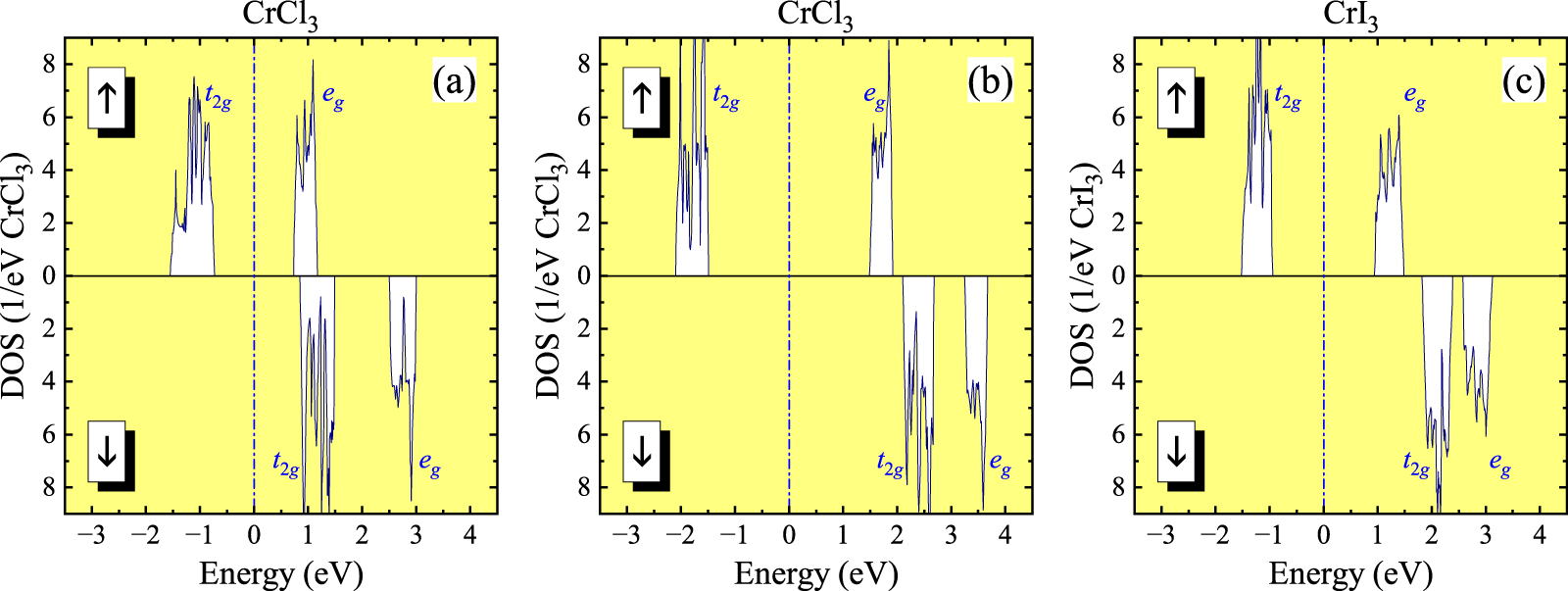
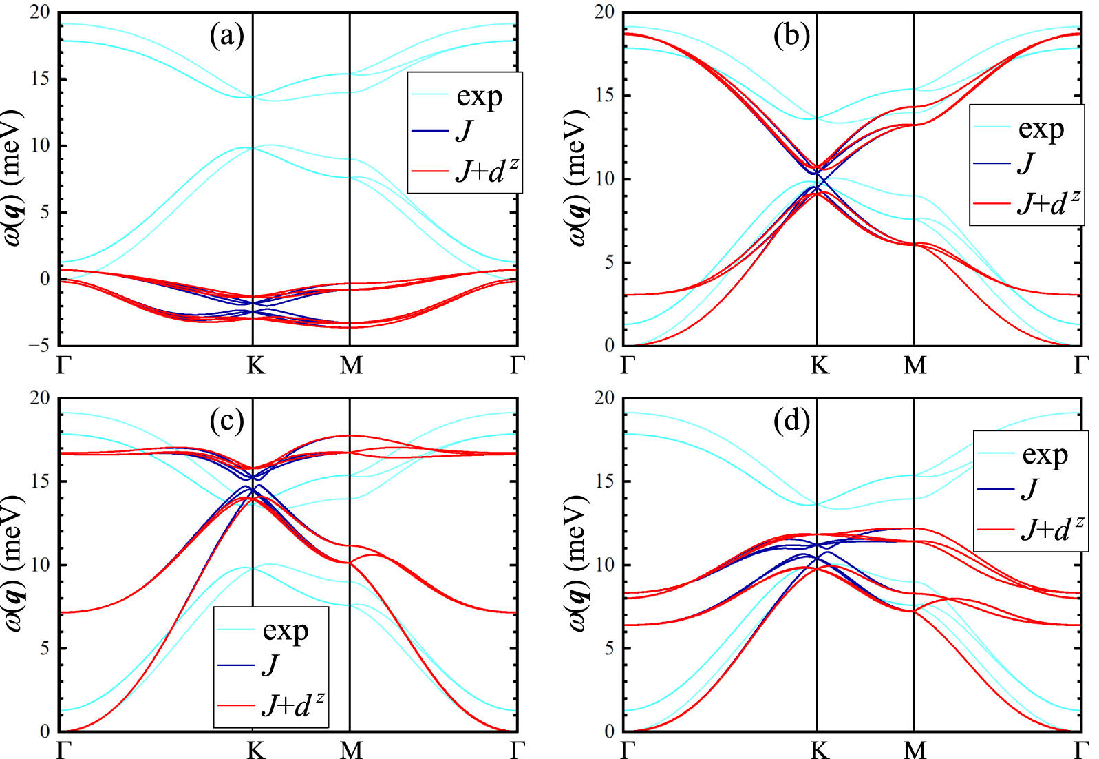
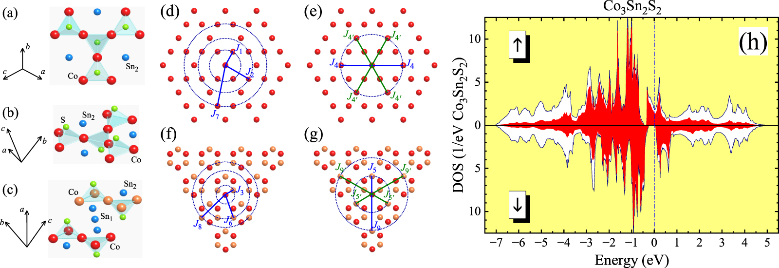
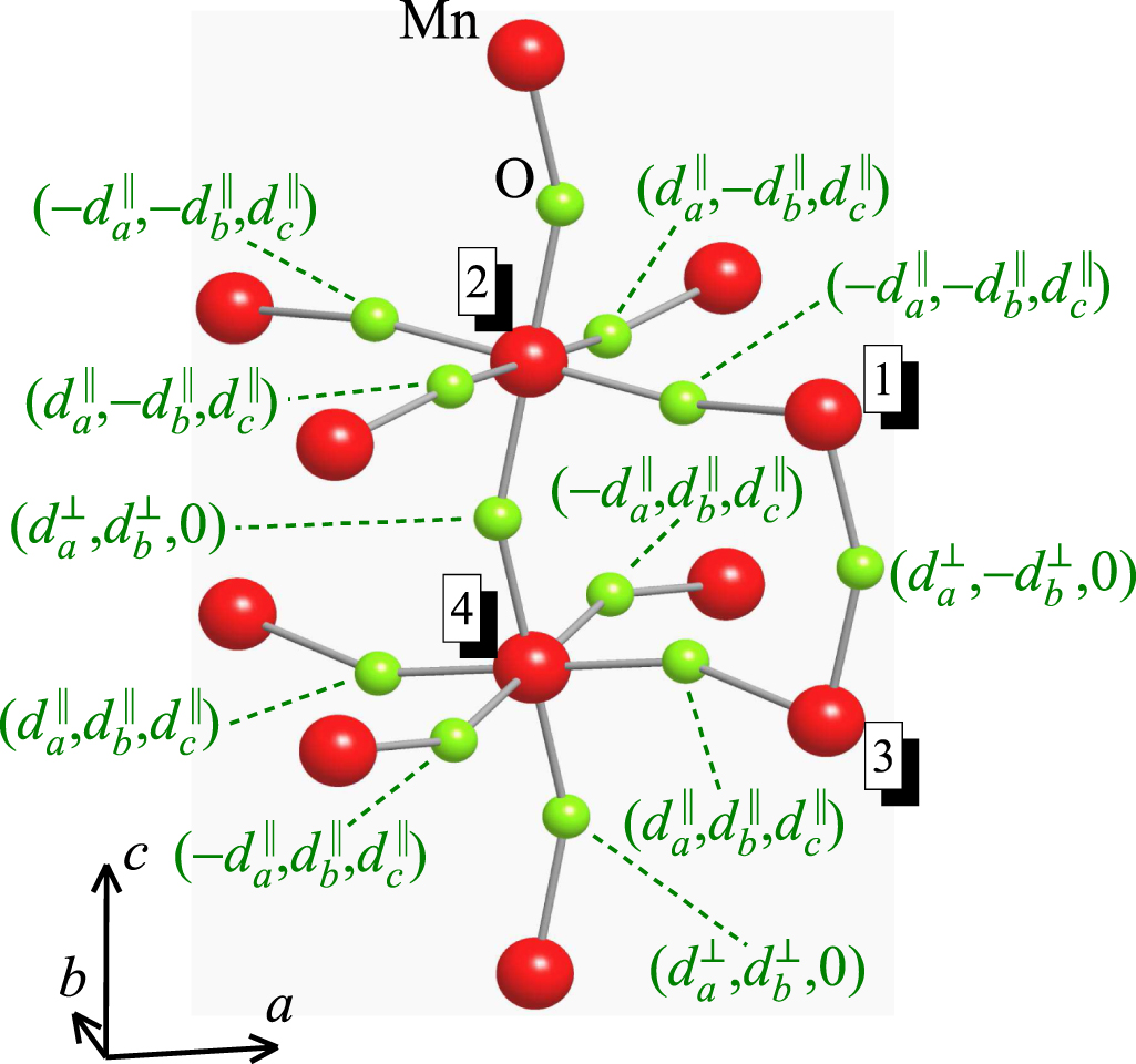