
Abstract
Magnetosensitive elastomers respond to external magnetic fields by changing their stiffness and shape. These effects result from interactions among magnetized inclusions that are embedded within an elastic matrix. Strong external magnetic fields induce internal restructuring, for example the formation of chain-like aggregates. However, such reconfigurations affect not only the overall mechanical properties of the elastomers but also the transport through such systems. We concentrate here on the transport of heat, that is thermal conductivity. For flat, thin model systems representing thin films or membranes and modeled by bead-spring discretizations, we evaluate the internal restructuring in response to magnetization of the particles. For each resulting configuration, we evaluate the associated thermal conductivity. We analyze the changes in heat transport as a function of the strength of magnetization, particle number, density of magnetizable particles (at fixed overall particle number), and aspect ratio of the system. We observe that varying any one of these parameters can induce pronounced changes in the bulk thermal conductivity. Our results motivate future experimental and theoretical studies of systems with magnetically tunable thermal but also electric conductivity—both of which have only rarely been addressed so far.
Export citation and abstract BibTeX RIS

Original content from this work may be used under the terms of the Creative Commons Attribution 4.0 license. Any further distribution of this work must maintain attribution to the author(s) and the title of the work, journal citation and DOI.
1. Introduction
Magnetosensitive elastomers are materials comprised of magnetizable inclusions embedded in an elastic carrier matrix [1–6]. The latter is usually a rubber or gel. Applying homogeneous external magnetic fields, the materials respond by changes in their overall properties. Most prominently, their stiffness and damping behavior, quantified in terms of static and dynamic mechanical moduli are affected [1, 6–12]. Similarly, shape changes occur in general, which is termed magnetostriction [13–17]. Both types of reaction illustrate how the materials sense magnetic variations in their environment. Possible applications therefore comprise tunable damping devices [18–20] and soft actuators [21–23], which are capable of a wider range of motion, such as jumping, walking, and rolling. Highly elastic magnetosensitive elastomers therefore are promising materials in soft robotics [20].
On a more microscopic level, an external magnetic field induces interactions between the magnetized inclusions. These interactions cause the inclusions to exert forces on and thus deform their elastic environment. Under sufficiently strong magnetic forces, the inclusions can substantially reorganize and rearrange themselves by deforming the elastic carrier matrix. For example, for two nearby particles, mutual attraction leading to their collapse towards virtual contact has been analyzed both theoretically [24–27] and experimentally [27]. Magnetically induced deformations and buckling of initially straight, chain-like aggregates were observed [28]. Specifically important for our considerations is internal restructuring leading to the formation of chains, which, likewise, have been reported in theoretical [11, 29, 30] and experimental [10, 31] studies. This effect has been correlated with changes in the elastic Young modulus of the materials of nearly an order of magnitude [10].
In the present work, we focus on the tunability of transport properties of such materials by external magnetic fields. Specifically, we concentrate on variations of heat transport through the system, as quantified by thermal conductivity.
Ferromagnetic fluids, a related class of materials composed of colloidal suspensions of magnetic particles in a carrier liquid, have been shown to exhibit increased thermal conductivity along the direction of an externally applied magnetic field and no changes in the conductivity in the direction perpendicular to the applied field [32, 33]. The change in thermal conductivity is reversible and decreases quickly once the magnetic field is turned off. Magnetic elastomers or gels designed to behave similarly in response to external fields could find medical application as a potentially biocompatible elastic carrier matrix. Compared to ferromagnetic fluids, soft elastic solids are generally more convenient to handle—requiring no container to hold them in place—and may be less susceptible to evaporation.
While there has been some research into the electrical conductivity of magnetosensitive elastomers, investigations focusing on thermal conductivity are still rarer. When homogeneous external magnetic fields are applied already during the curing process, chain-like aggregates form and are permanently imprinted in the materials [1, 34, 35]. The stronger the magnetic field during fabrication, the lower in general is the electric resistance [36–38]. Moreover, the chains can be separated or reconnected by stretching or compressing the material, which alters the electrical conductivity.
Thermal conductivity has been measured for a composite of carbonyl iron and agar [39]. There, again, the inclusions were aligned by an external magnetic field during curing, while stronger magnetic field amplitudes lead to larger thermal conductivity. The largest increase of thermal conductivity due to alignment was around 30% measured for a mass fraction of 10% carbonyl iron particles. Increasing the mass fraction of carbonyl iron increases thermal conductivity.
While there is some research on the electrical conductivity the main focus has been on materials with an already imprinted chain structure. However, in highly elastic elastomers and especially gels, these chains can also form when applying an external magnetic field after the curing process [29]. Here, the aim is studying the effect of this internal restructuring on the thermal conductivity.
In contrast to these works on prestructured materials, we here focus on systems that initially contain rather random arrangements of the magnetizable particles. We consider internal restructuring into anisotropic, mainly chain-like aggregates when external magnetic fields are applied. To this end, a coarse-grained bead-spring model is evaluated in two dimensions [11, 30]. We thus focus on the behavior of thin elastic films and membranes of magnetosensitive elastomers. In the restructured state under the influence of the external magnetic field, the change in thermal conductivity is evaluated as a function of the achieved magnetization of the magnetizable particles, their average distance, the overall particle number, and the aspect ratio of the rectangular system. Substantial tunability of the thermal conductivity is revealed.
We proceed as follows. In section 2, we present our theoretical model equations. Appropriate parameter values are selected in section 3. We describe how we evaluate the thermal conductivity in section 4. Our results for the variation of thermal conductivity as a function of the parameters mentioned above are provided in section 5. We conclude in section 6.
2. Bead-spring model for magnetosensitive elastomers
Our coarse-grained minimal model describes a mesh of springs with magnetizable beads connected to some of its nodes. The spherical beads represent the magnetizable inclusions and include the magnetic interactions [29], while the springs represent the elastic material behavior [40].
We start from a hexagonal network. During initialization, the position of each node is shifted by a random value chosen from a normal distribution of standard deviation of 10% of the lattice parameter  . Then, Nm
nodes are selected to associate to them the Nm
magnetizable beads. We place springs between any two nodes that are closer than 1.5 times the lattice parameter. An example system is depicted in figure 1. The top and bottom layers are not counted to the total amount of nodes, as they are not used in the calculation of the thermal conductivity (see below).
. Then, Nm
nodes are selected to associate to them the Nm
magnetizable beads. We place springs between any two nodes that are closer than 1.5 times the lattice parameter. An example system is depicted in figure 1. The top and bottom layers are not counted to the total amount of nodes, as they are not used in the calculation of the thermal conductivity (see below).
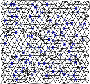
Figure 1. Example of a randomized hexagonal spring network with initial shifts of the nodes by a normal distribution of standard deviation of  , a lattice parameter
  , and a maximum spring length of
  . Springs (black lines) connect the nodes and magnetizable beads (blue circles) are randomly associated to the nodes. This example system features
  nodes and 100 magnetizable beads.
Download figure:
Standard image High-resolution imageBetween any two nodes i and j of positions  and
and  , respectively, the distance vector is defined via
  . Out of a total amount of nodes N, there are a number of Nm
magnetizable particles, all of diameter dc
. With the spring constant k, the elastic interaction potential is given by
. Out of a total amount of nodes N, there are a number of Nm
magnetizable particles, all of diameter dc
. With the spring constant k, the elastic interaction potential is given by
In this expression,  includes only pairs of nodes that are connected by springs, while
  sets the spring length in the undeformed state.
In the magnetized state, we always assume the external magnetic fields strong enough to approximately induce the saturation magnetization of magnitude MS in the magnetizable particles. In homogeneous external magnetic fields and for monodisperse particles, an identical magnetic dipole moment m arises for each particle, so that
As a result, we obtain the magnetic interaction potential [41]
where  ,
,  , and µ0 is the magnetic vacuum permeability.
Finally, the steric interaction potential between the beads is assumed as a modified version of the Weeks–Chandler–Andersen potential [11, 42]
Here, Θ denotes the Heaviside step function, while  and
and  depend on the exponents of Us
, in this case −6 and −12. Since Us
is always 0 if
depend on the exponents of Us
, in this case −6 and −12. Since Us
is always 0 if  , it is necessary to ensure a smooth transition and subsequent differentiability at
  . That means σs
and c are chosen so that
. That means σs
and c are chosen so that  and
and  are satisfied. εs
sets the magnitude of the steric interaction.
are satisfied. εs
sets the magnitude of the steric interaction.
To determine the new restructured states when magnetized, we assume overdamped dynamics of the nodes. For the equation of motion, combining  , we then obtain
with a damping coefficient ζ set equal for all nodes.  refers to the derivative with respect to the position of node i and t denotes time. As indicated above, we confine ourselves to two-dimensional evaluations representing thin sheets or membranes of magnetosensitive elastomers.
3. Rescaling of the basic equations and setting the system parameters
For the outlined description to represent real systems, it is necessary to choose appropriate values for the parameters. To find the actual number of independent parameters, we first rescale the equations in section 2 and then set realistic parameter values.
First, measure lengths in units of the diameter dc
of the magnetizable particles. Thus, distances become  . Energies are rescaled by
  , so that equations (1), (3) and (4) become
and
Here,  and
and  . Moreover, time is rescaled by
  , so that equation (5) reads
Thus, time becomes  with an incremental time step
  that we use to discretize equation (9) when we iterate it forward in time.
Now, there are only two dimensionless parameters remaining in equations (7) and (8) that control the system behavior. However, the role of the coefficient  in equation (8) for our purposes is simply to ensure sufficient volume exclusion of the particles. It is chosen large enough so that magnetized beads are generally not overlapping and low enough so that numerical stability is maintained. This leaves us with only one actual remaining system parameter, namely
in equation (7), where  is the Young modulus for three-dimensional systems. This scaled squared magnetic moment describes the relative strength of the magnetic versus the elastic interactions. To provide realistic results, this coefficient is approximated in the following on the basis of typical experimental data.
First, the saturation magnetization of carbonyl iron particles is around  [11, 43]. Average diameters for volume equivalent spheres of these particles reported in the literature are, for example,
  m for 15 wt % and 28 µm for 40 wt % samples [11].
The magnitude of the spring constant k for the spring network should reflect the magnitude of the elastic modulus of the underlying elastic material. In two dimensions (2D) it was shown that the Young modulus satisfies [44]
with λ and µ being the Lamé constants [44, 45]. The corresponding calculations were performed for uniaxial strain and stress. For a triangular lattice, the relation to the spring constant was found to be [44, 46]
Equations (11) and (12) are based on the hexagonal unit cell, see figure 2, of edge length b (in units of the bead diameter dc
) equal to the undeformed spring length. In the corresponding calculations these cells were assumed to have a thickness of  [46]. It follows with the respective units of
  and
and  as Nm−2 and Nm−1 that the relation between the three dimensional Young modulus
  and
and  is
is
Combining equations (11)–(13), we find
This relation, together with equation (2), justifies the second equality in equation (10). The typical Young modulus is of the order of magnitude  for a magnetic elastomer [10] and 1 Pa for a soft magnetic gel [28].
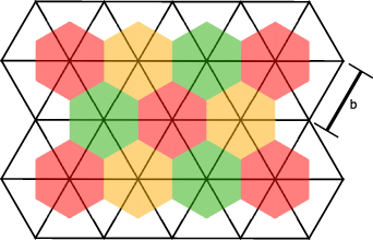
Figure 2. Regular hexagonal unit cells underlying the spring network to extract the relation between the spring constant k and the Young modulus  [46]. b denotes the length of the springs in units of the bead diameter dc
.
[46]. b denotes the length of the springs in units of the bead diameter dc
.
Download figure:
Standard image High-resolution imageThe Poisson ratio for elastic materials that are quantitatively described by the spring network is  [44, 46]. This means that our spring network represents a compressible medium. Different Poisson ratios can be achieved if angular interactions are added at the nodes connecting the springs [44, 46].
As we can see, the spring length b (in units of dc ) enters the expression for the remaining parameter Γ in equation (10). We will therefore include it into our considerations below. We approach b from the mass fraction ϕ of magnetizable particles in the medium, which we select as silicone rubber to set the associated parameter values [44].
We choose, for instance in figure 2, a unit cell with a node at the center that carries a magnetizable bead. As above, we assume the thickness of the sheet to be of size  . Thus, we obtain the following expression for the mass fraction using the volume
  of the magnetizable bead and the volume
  of the unit cell,
From there, we find together with  [47] and
  [48],
[48],
A sufficiently large number of magnetizable particles Nm
is necessary to facilitate chain formation upon magnetization. We therefore set the overall number ratio of beads and nodes  within the range of 25% and 50%. An approximate mass fraction ϕ from around 10% to 25% then implies a range of b from around 2 to 3.5.
4. Evaluation of the thermal conductivity
For each configuration and parameter setting, we iterate equation (9) forward in time using an Euler forward integration scheme until a steady state is reached. We then evaluate the thermal conductivity of the resulting configuration.
From the heat flux

where T is the local temperature and  denotes thermal conductivity [49], together with the conservation equation of thermal energy
where ρ is the (mass) density and c the specific heat capacity [50], we obtain the thermal diffusion equation
with  representing the thermal diffusivity [50].
The thermal conductivity of silicone can be found in the literature as  [51], its density as
  [47], and its specific heat capacity as
  [52]. The values for the magnetizable beads are chosen for iron carbonyl powder. We assume a density of
  [48], a thermal conductivity of
  [53], and a specific heat capacity of
  [39]. This leads to thermal diffusivities of
  and
and  , respectively.
To evaluate equation (19) in our situation, we employ an appropriate discretization of our system. We start from the nodes of our spring network and obtain discrete cells around them using a Voronoi tessellation [54]. We identify the temperature of each Voronoi cell with the temperature at the node that it contains. On this basis, we evaluate the heat flux between neighboring cells as described in the following. Corresponding quantities are introduced in figure 3.

Figure 3. Quantities used for the discretization to calculate the heat conduction between neighboring cells i and j are their 'volumes' Vi and Vj , respectively, absolute temperatures Ti and Tj , respectively, absolute contact 'area' Aij of the unit cells, and absolute distance lij between the central nodes.
Download figure:
Standard image High-resolution imageUsing Gauß' theorem, we obtain from equation (19) for the ith cell of 'volume' Vi
where  denotes the outward normal unit vector. Next, we assume constant temperature Ti
within the ith cell. According to equations (19) and (20), heat exchange with all cells
denotes the outward normal unit vector. Next, we assume constant temperature Ti
within the ith cell. According to equations (19) and (20), heat exchange with all cells  neighboring the ith cell can then be discretized as
Here, aij is the thermal diffusivity between cells i and j, Aij is their contact 'area', and lij is their distance, see figure 3. Thus, we find
Since this equation represents a discretized version of the heat equation, we expect conservation of heat, which we have confirmed in our numerical evaluations as described below.
To calculate the overall thermal conductivity, we induce an overall heat flux through the system. For this purpose, the temperatures of the boundary nodes on the left- and right-hand sides are fixed at  and
and  , respectively. Under these boundary conditions, the temperatures of all other nodes, here identified with the temperatures of the corresponding Voronoi cells, can then be found by iterating equation (22) forward in time. When a steady state is reached, the temperatures of all cells are constant in time,
  . This leaves us with
Equation (23) can be rewritten as a vector equation for all Voronoi cells as

where
T
c
is the vector of all temperatures of the boundary cells that are kept constant. The vector
T
v
contains all temperatures of the inner cells. The entries of the matrices
A
vv
and
A
vc
are extracted from the coefficients in equation (23). In fact, they constitute the negative discretized Laplacian operator for a graph with weighted edges [55]. We then calculate the temperature of each cell by solving equation (24) for  ,
,

In equation (23), the thermal conductivity λij
is set to  by default. It is only altered to λm
, when both cells i and j hold magnetized beads that are virtually in contact. Two beads are considered as being in contact when they are at most a center-to-center distance of
by default. It is only altered to λm
, when both cells i and j hold magnetized beads that are virtually in contact. Two beads are considered as being in contact when they are at most a center-to-center distance of  apart from each other. This corresponds to additional 4% of the effective steric radius and approximately corresponds to the magnitude of the numerical fluctuations observed for touching particles under strong magnetization. For illustration two examples for a system of
  nodes are displayed in figures 4 and 5. Here and in the following, we induce the magnetic dipole moments
m
along the negative overall temperature gradient.
nodes are displayed in figures 4 and 5. Here and in the following, we induce the magnetic dipole moments
m
along the negative overall temperature gradient.
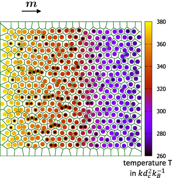
Figure 4. Heat conduction through a magnetized example bead-spring system of  nodes. Those nodes carrying magnetic beads are marked by black dots. Only little chain formation of magnetized beads has occurred in this case through the induced magnetic moments
m
oriented as indicated. Cell boundaries around the nodes as obtained from Voronoi tessellation are depicted by the dark lines. The temperature of each cell is indicated by the color scheme according to the scale on the right-hand side. (
nodes. Those nodes carrying magnetic beads are marked by black dots. Only little chain formation of magnetized beads has occurred in this case through the induced magnetic moments
m
oriented as indicated. Cell boundaries around the nodes as obtained from Voronoi tessellation are depicted by the dark lines. The temperature of each cell is indicated by the color scheme according to the scale on the right-hand side. ( denotes the Boltzmann constant.)
Download figure:
Standard image High-resolution image
Figure 5. Same as in figure 4, but for a system of substantial chain formation. The bright green circle outlines a region where the Voronoi cells around several nodes not carrying magnetizable beads are wedged between cells containing magnetizable beads. Still the surrounding beads are considered as being in contact due to their proximity.
Download figure:
Standard image High-resolution imageA special situation occurs when two magnetized beads are in contact but their Voronoi cells are not neighbors. Then, thermal conductivities involving the Voronoi cells  obstructing the connection will also be set to
  . This situation can occur when a cell not containing any magnetizable bead is wedged between two magnetized particles, see the configuration marked by a bright green circle on the right-hand side of the longest chain in figure 5.
The upper and lower rows of Voronoi cells in these figures do not contribute to the total amount of nodes N. They are excluded from the calculation of the thermal conductivity. Rather, they serve as purely auxiliary nodes to construct all Voronoi cells.
To now calculate the overall thermal conductivity of the entire system, we determine the total heat transported per time through a cross section A cutting through the whole sample perpendicular to the overall temperature gradient. We check that this transferred heat is identical through any cross section. The latter is required by conservation of thermal energy. Denoting by  all pairs of cells whose contact 'areas' Aij
together form the cross sectional 'areas' A, the total heat flux is calculated via
all pairs of cells whose contact 'areas' Aij
together form the cross sectional 'areas' A, the total heat flux is calculated via
At the same time, the overall thermal conductivity λ is defined via
where l is the averaged distance between the left and right boundary nodes. Combining equations (26) and (27), the overall thermal conductivity can be calculated as
The cross section A is averaged as well.  is calculated for as many cross sections as possible to verify conservation of heat.
Calculating l and A, averaging l and A, assuming a roughly rectangular shape of the system, and initially randomizing the placement of the nodes [56] all contribute to the error when determining λ. In our tests, we observed errors up to 6.1%, which is tolerable within the framework of our discussion.
We measure all thermal conductivities in units of  in order to highlight the relative change in conductivity due to magnetization, which in the initial system approximately equals
  by construction. Moreover, along these lines we eliminate the unit of thermal conductivity
  , which contains the unknown damping coefficient ζ.
5. Results
Using the implementation as described above, we evaluate the magnetically induced changes in overall thermal conductivity when we vary the scaled squared magnetic moment Γ, see equation (10), the average spring length b, the total number of magnetizable particles Nm , and the aspect ratio of the considered rectangular systems. In all cases, we magnetize the system from the initial, nonmagnetized state upon each change in the mentioned parameters. The internally restructured state is identified and the thermal conductivity is evaluated for each parameter setting separately. Additionally, we correlate the observed changes in overall thermal conductivity with the size of the generated chain-like clusters. We also briefly address the dynamics when the magnetization is turned on and off again.
5.1. Dependence on the relative strength of magnetic interactions Γ
We begin by considering the dependence of the overall thermal conductivity λ on the scaled squared magnetic moment Γ, see equation (10). For systems of  magnetizable beads randomly associated to the N = 400 nodes, we display in figure 6 results averaged over 50 realizations of the system (blue). A substantial increase of the overall thermal conductivity by a factor of approximately 4 is observed in a range of Γ that still corresponds to realistic parameter values. The averaged curve shows a nearly monotonic increase with Γ.
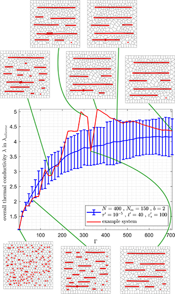
Figure 6. Overall thermal conductivity λ as a function of the scaled squared magnetic moment Γ averaged over 50 different realizations (blue line) of the system for  nodes, N = 400,
  , b = 2,
  , and
, and  , at
, at  . Standard deviations are marked by bars. Snapshots with the magnetizable particles in red and the Voronoi cells depicted in black are taken from one randomly selected example of the 50 systems. For that specific realization, we show the corresponding evolution of λ with increasing Γ as the red line.
Download figure:
Standard image High-resolution imageFor one selected example system, we additionally show in figure 6 the dependence of the overall thermal conductivity as a function of the strength of magnetic interactions Γ (red). Associated snapshots illustrate the formation of the aggregates with increasing Γ for this specific example. It demonstrates the tendency of increasing integration of magnetizable beads into chain-like structures when Γ rises. Naturally, the increasing magnetic interactions facilitate this reorganization against the restoring elastic spring forces. For sufficiently large values of Γ almost all magnetized beads are parts of large clusters and thus the thermal conductivity basically reaches saturation.
The sample system we depict in red is typical in that its thermal conductivity does not increase monotonically in Γ. This nonmonotonicity is the result of two distinct effects. First, with increasing Γ, beads that are in virtual contact increasingly overlap. The employed steric interaction potential is not perfectly hard and the steric interaction parameter  is finite. This overlap leads to an effective decrease in chain length when further increasing Γ. In reality, such effects may be observed if still some remaining soft material remains between the mechanically hard particles, for instance, for coated particles and/or absorbed polymer chains on their surfaces. Specific examples are provided by particles that serve as crosslinkers of the systems [57, 58]. A slight decrease in thermal conductivity may be associated with these effects, to which we attribute the gradual tapering off of λ in the high-Γ regime.
Second, the more pronounced steps of decrease on the red curve for the individual system in figure 6 can be of dynamic origin. We illustrate a corresponding scenario on a small example system of only  particles in figure 7.

Figure 7. For illustration, we consider a small example system of  magnetizable beads. The panels on the left-hand side show the final states upon chain formation for different strengths of magnetic interaction (a)
  , (b)
, (b)  , and (c)
  . In these snapshots, blue spheres represent the magnetized beads and the black mesh corresponds to the boundaries of the Voronoi cells. Associated panels on the right-hand side depict the trajectories of the individual nodes, where brightening colors represent progression in time.
Download figure:
Standard image High-resolution imageIn figure 7(a), for  , smaller chains of 3 magnetized beads form, besides one remaining separate bead and another chain of 5 beads, leading to an overall thermal conductivity of
  . Further aggregation is prevented as the necessary magnetic interactions cannot overcome the prevailing elastic interactions. These elastic interactions are partially overcome when the magnetic interactions are increased to
  , see figure 7(b), when significantly longer chains of 5 and 7 beads form. As a consequence, the thermal conductivity increases to
  . However, at still larger
  in figure 7(c), the overall thermal conductivity again drops to a lower value of
  . This lower value is correlated with on average two shorter chains of only 5 beads and two remaining separated beads.
To understand this behavior, we recall that, for each value of Γ, the system is initiated in a nonmagnetized state. Then the beads are magnetized. The speed of the subsequent dynamics increases with Γ. For  , quicker contraction implies that the outer beads cannot follow the quick displacement of the inner beads when the upper chain in figure 7(c) is formed. This is different for the slower dynamics in figure 7(b) for lower Γ. The more separated structures in figure 7(c) correlate with a reduced overall thermal conductivity for
  when compared to
  . The two separate particles remain separated because the distances to the other particles are too large and thus the magnetic attractions are too weak to overcome the elastic counterforces. Thus, on the side, we conjecture that the protocol of introducing the magnetization can influence the resulting internal structure. It may thus represent another means of tailoring the resulting thermal conductivity.
As can be inferred from the right panel for  in figure 7(c), the separated magnetizable bead on the right-hand side even turns around while the aggregation dynamics is in progress. This happens at the time when the upper and lower chains form quickly and the particles within the quickly formed chains are already too far apart to induce significant attraction.
In contrast to that, the averaged curve for a larger system size in figure 6 does not exhibit any sharp elevations in thermal conductivity any more. While there are some nonmonotonic intervals, there are not any significant spikes outside the given standard deviation.
5.2. Impact of the average scaled spring length b
First, we recall that the initial spring network corresponds to a randomized hexagonal arrangement. Therefore, we refer to the averaged spring length b in this system. Second, b is measured in units of dc and thus represents a relative, dimensionless parameter. The relation between b and the mass fraction ϕ was given in equation (16).
Figure 8 displays the overall thermal conductivity as a function of the spring length b when averaged over 50 different realizations of the system at an elevated magnitude of magnetization. All other parameters, including the total number of magnetizable particles and aspect ratio of the systems are kept fixed. The decrease in thermal conductivity for increasing relative spring length b is apparent.
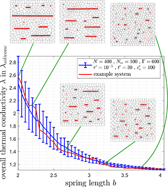
Figure 8. Overall thermal conductivity λ as a function of the relative spring length b (measured in units of the bead diameter dc
) averaged over 50 realizations of the system of  nodes for N = 400,
  ,
,  ,
,  , and
, and  , at
, at  . Snapshots for one randomly selected realization with the magnetizable beads indicated in red and the Voronoi cells depicted in black are included as insets.
Download figure:
Standard image High-resolution imageThe reason for this decrease is inferred from the snapshots added as insets in figure 8 for one specific example realization. For lower values of b, corresponding to increased densities of the magnetizable particles, the system is able to form elongated chain-like clusters. Due to the small initial distances between the magnetized beads, mutual magnetic interactions are strong and the elastic counterforces are easily overcome. We recall that the strength of magnetic dipole interaction scales as the inverse cubic interparticle distance, see equation (3). With increasing relative spring length b, the average initial distance between nearest neighboring beads is larger and the same magnetic moment may not be sufficient any longer to induce cluster formation. This effect is clearly visible from the insets in figure 8 corresponding to an elevated spring length b.
5.3. Dependence on the number of magnetizable particles Nm
Along analogous lines as above, figure 9 displays the overall thermal conductivity λ as a function of the number of magnetizable particles Nm , while all other parameters remain fixed. The curve displays some nonmonotonic steps, see also the discussion in section 5.1, yet well within the range of the standard deviations. Thus, as a general trend, the thermal conductivity rises with increasing numbers of magnetizable particles as expected. The snapshots in figure 9 taken for one specific example realization illustrate that generally the lengths of the formed chain-like aggregates increases with increasing Nm , which supports overall heat transport through the system.
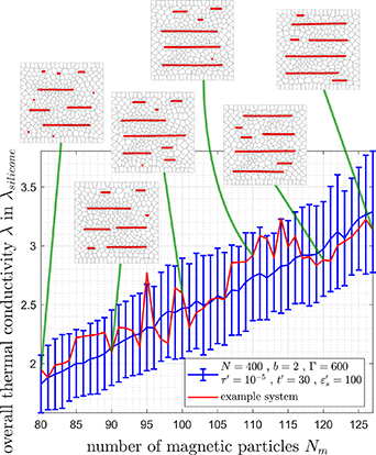
Figure 9. Overall thermal conductivity λ as a function of the number Nm
of magnetizable particles averaged over 50 realizations of systems of  nodes for N = 400, b = 2,
  ,
,  , and
, and  , at
, at  . As insets, we include snapshots for one randomly chosen system, where we indicate the magnetizable beads in red and the boundaries of the Voronoi cells in black.
Download figure:
Standard image High-resolution image5.4. Effect of the aspect ratio
All the data in sections 5.1–5.3 were obtained for initially square-like systems of  nodes. To get an impression of the relevance of this shape, we vary the aspect ratio to other rectangular contours. Figure 10 depicts selected example systems of (a)
  nodes (longest system), (b)
  nodes (long system), (c)
  nodes (square system), (d)
  nodes (wide system), and (e)
  nodes (widest system). The remaining parameter values were all kept identical in the different situations.
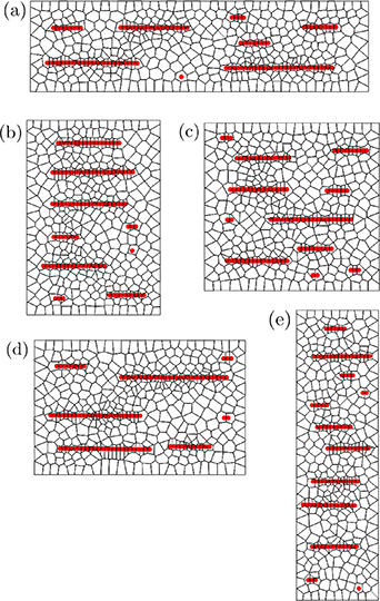
Figure 10. Example systems of different aspect ratios but otherwise identical parameter settings. Specifically, we address systems of (a)  nodes (longest system), (b)
  nodes (long system), (c)
  nodes (square system, see sections 5.1–5.3), (d)
  nodes (wide system), and (e)
  nodes. The snapshots show the systems in the magnetized state for scaled squared magnetic moment
  , relative spring length b = 2, number of magnetizable particles
  , strength of steric interactions
  , and incremental timestep
  at
at  .
.
Download figure:
Standard image High-resolution imageThe overall thermal conductivities for systems elongated along the overall thermal gradient are displayed in figure 11, where for each aspect ratio we again average over 50 different realizations. There, the values of the overall thermal conductivity are virtually the same as in the square system. However, their standard deviation substantially increases with elongated systems. Since the systems are slimmer perpendicular to the direction of magnetization, in some individual systems an exceptionally long chain-like aggregate forms. Such individual occurrences significantly increase the thermal conductivity and thus the standard deviation.
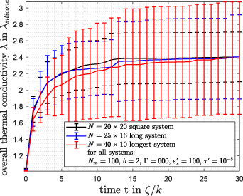
Figure 11. Overall thermal conductivity λ as a function of time for initially square-shaped systems and systems initially elongated along the magnetization direction. Again, we average over 50 different realizations for each aspect ratio.
Download figure:
Standard image High-resolution imageIn contrast to that, figure 12 shows results for systems that are initially wider perpendicular to the magnetization direction. For wider aspect ratios, the averaged overall thermal conductivity decreases, but remains within the standard deviation. Since the systems are shorter along the magnetization direction, the maximum length of the chain-like aggregates is reduced.
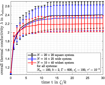
Figure 12. Overall thermal conductivity λ as a function of time for initially square-shaped systems and systems initially shorter along the magnetization direction, averaged over 50 different realizations for each aspect ratio.
Download figure:
Standard image High-resolution image5.5. Correlation with the average cluster size
In addition, we correlate the magnetically induced changes in the overall thermal conductivity λ with the average size of the formed chain-like clusters. To this end, we reconsidered the above examples of square-shaped systems and the averages over 50 realizations as displayed in figures 6, 8, and 9, that is, for increasing strength of magnetic interaction Γ, relative spring length b, and total number of magnetizable beads Nm , respectively. The size of a cluster is defined as the total number of beads that are in virtual contact with each other. The average cluster sizes were obtained by first averaging the sizes of all clusters in each realization and subsequently over the 50 different realizations. Associated standard deviations depicted below are associated with the second averaging step.
Our results are summarized by figure 13. In all cases, an increase in average cluster size is related to an increase in thermal conductivity. The average cluster size and thus the thermal conductivity increases with increasing scaled squared magnetic moment Γ, see figure 13(a), decreasing relative spring length b, see figure 13(b), and increasing total number of magnetizable particles Nm , figure 13(c).

Figure 13. Correlation between the average size of the formed chain-like clusters and the magnetically induced change in overall thermal conductivity λ. Results are shown for increasing (a) scaled squared magnetic moment Γ, (b) relative spring length b, and (c) total number of magnetizable particles Nm , see the color codes on the right-hand sides. Again, we average over 50 realizations of each system. The data correspond to our results in figures 6, 8, and 9, respectively.
Download figure:
Standard image High-resolution imageWe add a remark concerning the leveling slope of the curve in figure 13(a) at elevated strengths of magnetic interactions Γ. This effect is partially linked to imperfections that arise during the magnetically induced aggregation. The clusters do not necessarily feature a perfect chain-like structure, as illustrated on the example in figure 14. First, when a shorter chain approaches a longer chain obliquely from the side, the shorter chain may laterally dock and attach to the longer one. Due to the magnetic attraction within the longer chain, the smaller chain is prevented from being absorbed into the longer chain. Examples are displayed in figure 14 as marked by the green circles. Second, two longer chain-like clusters may connect while partially overlapping side by side. A corresponding resulting structure is depicted in figure 14 as marked by the blueish circle.

Figure 14. Snapshot of a chain-like cluster formed upon magnetization. It contains two types of imperfections. One type refers to smaller chain-like aggregates attached to the side, as marked by the left two (greenish) circles. The other type implies imperfectly joined chains that partially overlap, as marked by the right (blueish) circle. (Parameter settings:  nodes,
  , b = 1.7,
  ,
,  ,
,  ,
,  .)
.)
Download figure:
Standard image High-resolution image5.6. Dynamical aspects when switching on and off the magnetization
Our basic dynamic equations equation (5) in our investigation serve to find the final static state upon magnetization. In this simplified form, they are not suited to quantitatively extract details of the underlying dynamic processes themselves. Nevertheless, a simple qualitative insight is provided.
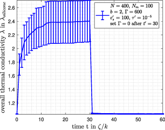
Figure 15 displays the time evolution of the overall thermal conductivity when at t = 0 the beads are magnetized to  , while at
  their magnetization is switched off again.
Figure 15. Overall thermal conductivity λ as a function of time when averaged over 50 realizations of a system of  nodes. Magnetization is induced at t = 0, while it is switched off again at
  .
.
Download figure:
Standard image High-resolution image
Interestingly, it takes a while until the saturation value of the thermal conductivity is reached, while it quickly drops towards zero when magnetization is switched off. The longer initial procedure can be explained by the coarsening process when the large chain-like clusters form upon magnetization. Initially formed smaller clusters need to migrate collectively as larger objects to assemble into larger chain-like structures over time. In contrast to that, when the magnetization drops to zero, each particle individually is driven by the restoring elastic forces to find back into a separated arrangement.
6. Conclusions
In this work, we analyzed the magnetically induced changes of thermal conductivity in thin films or membranes of magnetosensitive elastomers. To this end, we employed a simple yet effective bead-spring model. Magnetizable inclusions are represented by spherical beads randomly placed on the nodes of a randomized hexagonal spring network. The latter represents the underlying elastic interactions in the material.
Upon magnetization, depending on the strength of the induced magnetic interactions relative to the mechanical stiffness, internal restructuring occurs. Particularly, chain-like particle aggregates form. We determine the changes in overall thermal conductivity resulting from the internal restructuring. The rearrangement of the magnetizable particles can lead to a substantial increase of thermal conductivity along the magnetic field direction.
Along these lines, we studied the consequences of varying the scaled squared induced magnetic moments of the beads, the lengths of the springs forming the elastic network, the number of magnetizable particles, and the aspect ratio of the rectangular network structure. Individual systems may display nonmonotonic behavior when altering one of the aforementioned quantities. Yet, the behavior generally smoothens out on average.
Increasing the scaled squared magnetic moment, which relates the strength of the magnetic interactions to the elastic stiffness, causes an increase in thermal conductivity associated with increasing lengths of the chain-like aggregates, until a saturation level is reached. Conversely, an increasing spring length, which is related to the volume fraction of magnetizable particles, causes the thermal conductivity to drop, while the overall system size increases. For a low spring length, large clusters form, with an increased amount of imperfections in the chain-like structure. In that case, the distances between the magnetizable particles are so small that the resulting modified dynamics counteracts proper alignment in perfect particle chains. Generally, an increase in the volume fraction of magnetizable particles causes an increase in thermal conductivity, while we have not observed a substantial effect of the aspect ratio. We further supported our results by relating the variations of thermal conductivity as induced by changes in the mentioned parameters to changes in the averaged cluster size. A qualitative consideration of the dynamics of the system indicates that cluster formation and the associated increase in thermal conductivity upon magnetization occur significantly slower than cluster dissociation and decrease of thermal conductivity when the particles are demagnetized.
In future investigations, the discretization into a spring network and the associated Voronoi tessellation into discrete cells could be refined. Specifically, individual particles could be represented by multiple Voronoi cells of higher thermal conductivity. Additionally, the bead diameters could be varied to represent conditions of polydisperse particle distributions. The influence of the magnetization protocol on the resulting structures and thermal conductivity should be analyzed. Besides, in nonuniform magnetic fields, additional translational forces emerge. Finally, the description so far has only addressed thin flat systems, representing thin films and membranes of magnetosensitive elastomers. Extensions to three-dimensional systems appear desirable.
Overall, we hope that our study will further motivate investigations on the promising magnetically tunable transport properties of magnetosensitive elastomers. So far, some studies on the electric conductivity [36–38] and a few on the thermal conductivity [39, 59] have been reported for these materials. Both on the experimental and on the theoretical side, a lot of future work is still in order to fully understand the resulting types of behavior. This includes microscopic aspects of thermal coupling between individual polymer chains and the particle surfaces. The results will be important both from a fundamental and applied perspective.
Acknowledgments
The authors thank the German Research Foundation (Deutsche Forschungsgemeinschaft, DFG) for support of this work through the SPP 1681 via Project No. ME 3571/3-3 (G J L J, L F) and through the Research Grant No. ME 3571/5-1 (T L). A M M acknowledges support by the DFG through the Heisenberg Grant No. ME 3571/4-1.
Data availability statement
The data that support the findings of this study are presented as data points in the figures and are available upon reasonable request from the authors. The data that support the findings of this study are available upon reasonable request from the authors.