
Abstract
In this work we show the calculation of optimized efficiencies of intermediate band solar cells (IBSCs) based on Mn-doped II-VI CdTe/CdMnTe coupled quantum dot (QD) structures. We focus our attention on the combined effects of geometrical and Mn-doping parameters on optical properties and solar cell efficiency. In the framework of  theory, we accomplish detailed calculations of electronic structure, transition energies, optical selection rules and their corresponding intra- and interband oscillator strengths. With these results and by following the intermediate band model, we have developed a strategy which allows us to find optimal photovoltaic efficiency values. We also show that the effects of band admixture which can lead to degradation of optical transitions and reduction of efficiency can be partly minimized by a careful selection of the structural parameters and Mn-concentration. Thus, the improvement of band engineering is mandatory for any practical implementation of QD systems as IBSC hardware. Finally, our calculations show that it is possible to reach significant efficiency, up to ∼26%, by selecting a restricted space of parameters such as quantum dot size and shape and Mn-concentration effects, to improve the modulation of optical absorption in the structures.
Export citation and abstract BibTeX RIS
1. Introduction
Intermediate band solar cells [1–4] (IBSCs) are high efficiency solar cell structures based on the engineering of an intermediate band (IB) between the valence band (VB) and conduction band (CB) of a semiconductor material. The IB produces an increase in photocurrent through two-photon absorption processes, where a single photon promotes an electron from the VB to the IB level and the second photon promotes an electron from the IB to the CB, thus creating a single electron–hole pair [1, 5]. Under optimum conditions and within the theoretical frame of the detailed balance method (DBM), IBSC configuration may reach efficiency of ∼60%, surpassing the Shockley–Queisser limit [1]. Experimentally, IBSC systems can be achieved even by using highly mismatched semiconductor alloys, or diluted magnetic semiconductors (DMS) and quantum dot arrays. A detailed presentation of current efforts on the experimental realization of IBSC can be found in the review by Okada et al [2].
Semiconductor quantum dots are nanostructured systems where the position of a discrete energy level can be engineered by the manipulation of parameters such as size, shape, stress or by an appropriate choice of materials forming the structure. Moreover, advances in epitaxial growth techniques have enabled the fabrication of vertically aligned coupled dot structures, also known as quantum dot molecules (QDMs), in which the formation of delocalized states enables new interdot optical transitions. These structures, referred to as man-made molecules, have demanded great interest because of their potential applications as optoelectronic devices or even as quantum computing systems. In this context, solar cell devices that explore the positioning of discrete energy levels of quantum dots (QDs) to form an IB within the band-gap of the host material can be viewed as possible physical realizations for the IBSC. Based on simple QD models, an efficiency of about 63% has been predicted for QD-IBSC [6].
Currently, the search for manipulated materials that may provide optimal efficiency in photovoltaic energy conversion is one of the most important challenges in QD-IBSC technology. A myriad of binary compounds and ternary alloys and their nanostructures has been suggested for the implementation of the QD-IBSC and, among them, we can mention: self assembled QDs as InAs/AlGaAs [7], ternary alloys based on type InGaAs/GaAs, InGaAs/GaAsP [8], wide-bandgap materials as InAs/InGaP [9], colloidal QDs based on CdSe [10], type II CdTe/CdSe core/shell QDs [11] and colloidal n-type PbS [12] QDs, which has been proposed as an environment to IBSC based on QD.
As mentioned by Popescu et al [8], several conditions must be established for a successful implementation of the IBSC based on dots, which involves the precise control of the intermediate energy band position and the optimization of the interband gap optical absorption processes. In this context, controlled doping techniques [13], manipulation of geometric QD parameters and band realignment engineering [11, 14] are important tools in the search for improved best efficiencies of photovoltaic energy conversion systems. A schematic type QD structure and the relevant energy levels for this work are shown in figure 1.
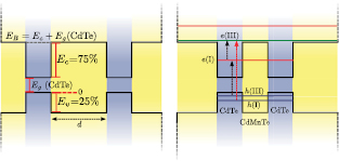
Figure 1. Schematic representation of the coupled QD system. The interdot separation is labeled as d. The left panel shows the conduction-VB offset ratio of 75:25 used for the CdTe–CdMnTe interface, the dashed gray line represents the electron barrier height given by  . The right panel shows the intermediate conduction state
  and the extended CB states
  in the discretized or quasi-continuum set of levels determined by the length of the outsider barriers of the QDM structure. The vertical dashed arrows indicate the relevant allowed intraband and interband optical transitions.
Download figure:
Standard image High-resolution imageIn this paper, we concentrate our efforts on the search for a clear understanding of intra- and interband optical transitions in QDs as key ingredients in photovoltaic conversion efficiency. For a better description of the transitions between bound states (BS), associated with the presence of the QD, and between bound and extended states (ES) in the CB, we use the multiband  method to calculate energy level structures. Single-band approximations do not include important effects such as band admixture or band symmetries, and thus do not provide reliable description of the optical transitions oscillator strengths. On the other hand, the choice of a QD system that allows great flexibility in the manipulation of optical absorption properties is also important. As we have shown in previous works [15, 16], a system with highly controllable optical properties is formed by II–VI QDs doped with Mn magnetic ions in the dilute magnetic semicondutor (DMS) regime. In this system, it is possible to improve the controllability of the energy level positions considering a configuration of finite barrier double QDs separated by a Mn-doped barrier. The influence of Mn-doping on the quantum efficiency of CdS [13] and CdMnSe [17] QDs, within the solar cell context, has recently been discussed.
The system proposed here is formed by two identical CdTe QDs coupled through a Mn-doped  MnxTe barrier. We will discuss in detail the effects of structural parameters such as QD radius and interdot separation on the optical parameters, determining transition oscillator strengths and photovoltaic energy conversion efficiencies. Special attention will be devoted to studying the interplay between Mn concentration and structural parameters in order to find conditions to reach optimized efficiencies.
2. Theory
We consider a system composed of two identical vertically coupled CdTe QDs of radius R and height hz separated by a semimagnetic  MnxTe barrier of width d, as shown in figure 1. The growth direction z is chosen as the quantization axis for the angular momentum. Following the effective mass approximation, we describe a carrier in the presence of a confinement potential V from the solutions of the Schrödinger equation
  for the eight-component spinor ψ. We have chosen to use the complete 8
  8
8  Kane-Weiler model [18], which takes into account the known interactions between states near the
  ,
,  and
and  bands exactly and considers contributions from remote bands. The detailed form of
  Hamiltonian is reported in [18]. In general, each component of the spinor has the form
  , where
  is a normalization constant,
  is the Bessel function and
 ![$f^{\pm}(m, z)=\frac{1}{\sqrt{H_z}} \sin[m\pi(\frac{1}{2}-\frac{z}{H_z})]$](https://content.cld.iop.org/journals/0953-8984/29/44/445301/revision2/cmaa85c7ieqn018.gif) . Here Hz is the normalization length in the z-direction and the upper (lower) sign in
. Here Hz is the normalization length in the z-direction and the upper (lower) sign in  corresponds to m even (odd) symmetry, respectively.
As a consequence of the axial symmetry, the z-component of the total angular momentum can be introduced as a good quantum number. The z projection of the angular momentum can be written as  , where Jz is the z-component of the angular momentum of the edge Bloch function and Lz is the z-component of the envelope angular momentum [19]. The wave functions
  and
and  for subspaces
  and
and  of different parities can be written as a linear combination of the envelopes
  and the eight Bloch functions at the
  -point, as
for Hilbert subspaces I and II, and
for Hilbert subspaces III and IV. In these expressions,  are constants to be determined from diagonalization. The Hilbert subspaces
  and
and  are degenerate as well as subspaces
  and
and  .
.
The optical transition probability is proportional to the matrix element of the crystal radiation field interaction  , where
  = I(II), III(IV). Here
  is the light polarization vector and
  is the momentum operator. Using equations (1) and (2), the above matrix element can be written as

Here, the conduction (valence) band states are  (
( ), with α labeling the corresponding quantum numbers
  and the periodic Bloch functions at the Γ-point of the Brillouin zone,
  , following the same ordering as in equations (1) and (2).
For interband transitions, only the first term in equation (3) contributes to the overlap integral, which can be separated into integrations over the fast oscillating Bloch part that will determine the interband selection rules, and integrations over the envelope part that determine the intensities of the transitions proportional to the oscillator strengths. The integrations of the Bloch function part result in the size-independent dipole matrix elements that will be named  . The complete set of selection rules are obtained from the non-vanishing products of the matrix elements
  , where
  are the envelope overlap integrals.
Due the different symmetry of the electron and hole angular momentum, the allowed interband transitions are those between initial and final levels belonging to different Hilbert subspaces, i.e. transitions between VB  to CB subspaces
  . We can determinate the selection rules for unpolarized normally incident light thus, we take the time average between x- and y-polarizations such as
Here, the right (+) and left (−) circular polarizations are  , respectively. Moreover, for the quantum numbers m and L, we have
  and
and  for the light polarization
  , respectively.
For the  , the optical matrix element (3) takes the form

where
with  .
.
The second term in equation (3) contributes to intraband transitions between intermediate and CB levels. Here, only transitions between levels with the same spin orientation and belonging to different Hilbert subspaces,  , are allowed. These selection rules can be labeled as
  and
and  for the light polarization
  , respectively. The intraband oscillator strength for these transitions is given by

In order to discuss the optical absorption spectra, the interband oscillator strength  between single electron
  and hole
  states and intraband oscillator strength
  between electron in the IB and electron in CB, has to be evaluated in detail. The absorption coefficient involves transitions between VBs and IBs, then to the quasi-continuum CB levels and this can be cast as
In these expressions, we have neglected the effects of nonhomogeneous broadening and assumed a constant broadening value Γ for all optical transitions, with  being a constant, η being the refractive index and ω the incident light frequency.
The photocurrent density has been calculated by using [5, 20]

where  is the thickness of the active absorbing media, α is the overall optical absorption which involves transitions from VB to IB, then to CB, where
  is the spectral solar flux modeled from black-body radiation at the sun temperature TS. The efficiency η of the solar cell is defined by the ratio between the power output delivered by the cell to the power output of the sun incident illumination on the cell. The power of the sun, PS, is constant and related to the sun temperature TS, and the geometrical factor F, which accounts for angular dependence of radiation, and defined as:
  , where θ is the angle subtended by the sunlight. A circuit delivers a power density that is described by
  , where J is the current density at given voltage V. Thus, the determination of the efficiency
  is directly linked to a proper calculation of current density J of the system. Some assumptions should be made in order to calculate the current density: (i) sun and solar cells behave like black-body systems at different temperatures, (ii) direct radiative transitions are dominant and nonradiative transitions are ignored, (iii) all photons with energy above the band gap Eg are absorbed, (iv) quasi-Fermi levels are constant,
  , (v) a single electron–hole pair is created per absorbed photon, and finally vi) maximum concentration of sunlight is assumed, corresponding to cell illuminated with
  , thus
  [21].
[21].
3. Results
In order to calculate the electronic structure based on the multiband  method, we use the following set of parameters [22]: the Luttinger parameters
  ,
,  ,
,  , the CB effective mass for CdTe
  , spin–orbit splitting energy
  meV, CdTe band gap taken at
  K,
K,  meV and Kane conduction-VB coupling:
  eV. Additionally, we consider the Mn-concentration dependence of the CdMnTe band gap as
  meV. This relation was obtained after the linear fitting of experimental results [22]. The conduction-VB offset for the CdTe-CdMnTe interface is a critical parameter once it will define the QD intermediary band position. In our case we use:
  , where
  and
and  .
.
Before presenting our results, we briefly explain our calculation strategy. The number of electronic levels in a QDM structure strongly depends on structural parameters such as the QD radius R, QD height hz and the overall vertical size Hz. A bad choice of these parameters may lead to a dense spectrum of energy levels that, eventually, could degrade the optical absorption of the system. To avoid this adverse effect, we restrict the number of energy levels in the CB to just two levels: the localized IB  and the extended quasi-continuous level
  as shown in figure 1, respectively. To achieve this precise level configuration, we calculate the energy spectrum for fixed values of Hz and hz, considering the QD radius R as an independent parameter. Next, we carefully select the range of radii values that only allows one to accommodate a single electron level
  in the QD. The extended state
  is approximately resonant to the barrier energy
  . This procedure is repeated for each value of the Mn-concentration x and interdot separation d. In order to exemplify our calculation scheme, the figure 2 shows the energy spectrum for a CdTe/CdMnTe QDM as a function of
  for two different values of the interdot separation d. The remaining structural parameters Hz, hz and the Mn-concentration x were kept constant.
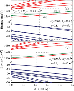
Figure 2. Energy spectrum for the CdTe/CdMnTe QDM as a function of the inverse of the QD radius  , for two values of the interdot separation
  and
and  . In all cases, the Mn-concentration and the structural parameters Hz and hz remained fixed. Red lines (blue lines) represent the conduction (valence) band level structure. The conduction level (green line) represents the extended conduction state
  . The thick horizontal gray line identifies the barrier height for electrons and the rectangular dashed line selects the set of conduction and valence levels relevant for this study.
Download figure:
Standard image High-resolution imageThe thick horizontal solid gray-line represents the electron barrier height  meV, for Mn concentration
  . The lowest electron level is denoted as
  (lowest solid red line) and corresponds to the IB. The branch state shown by the green line,
  , is the first of the extended states, which is a part of the quasi-continuum CB for
  . The dashed-line rectangular region selects the important set of CB and VB states in our study and, in the sequence, we will focus on the interval
 ![$[R_{{\rm min}}, R_{{\rm max}}]$](https://content.cld.iop.org/journals/0953-8984/29/44/445301/revision2/cmaa85c7ieqn096.gif) defining the width of this rectangular region. Here,
defining the width of this rectangular region. Here,  corresponds to a QD radius for which the IB state
  is resonant with the energy barrier EB and the Rmax corresponds to the first state,
  , closest to the resonant situation EB in the extended region. Finally, we calculate the solar cell efficiency η within each interval
 ![$[R_{{\rm min}}, R_{{\rm max}}]$](https://content.cld.iop.org/journals/0953-8984/29/44/445301/revision2/cmaa85c7ieqn100.gif) and select the set of radii dot values that maximize η.
and select the set of radii dot values that maximize η.
Now we return to the analysis of figure 2 for these considered cases. First, a strongly hybridization of the valence and CBs as the interdot separation d becomes larger can be noticed. This behavior is characteristic of all molecular systems, but becomes more dramatic in QDs, where the quantum confinement and external fields cause strong level admixtures particularly important in the VB. As our system also includes a region of quasi-continuum extended states very close to each other in energy, we also expect the emergence of strong CB admixtures. These combined situations lead to a relaxation of the optical selection rules and should reduce solar cell efficiency. This assertion will be numerically proved later.
Following our calculation scheme discussed above, we show in figures 3(a) and (b) the interband and intraband transition energies as a function of QD separation d for three different values of Mn concentration x and  , and
, and  . It is important to recall that each point in these figures is calculated for a specific radius value which maximizes the efficiency η. To illustrate this, we include in figure 3(c) the maximum efficiency values (lower number) and their corresponding radii (upper number), obtained according to our calculation procedure. This information will be useful for further discussion. For the same set of structural parameters we show the interband and intraband oscillator strengths as a function of d in panels (c) and (d).
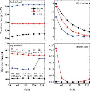
Figure 3. (a) Interband ( ) and (b) intraband (
 ) transition energies as a function of interdot separation d for different values of Mn-concentration x. (c) Interband
  , and (d) intraband
  optical oscillator strength as a function of d for different values of Mn concentration. In all cases, the structural parameters are
  , and
, and  . The lower and upper numbers in panel (c) represent the maximum efficiencies and their corresponding radius, respectively. The solid lines are guides for the eyes.
Download figure:
Standard image High-resolution imageAs seen in figure 3(a), interband  energy transition is highly sensitive to an increase in Mn concentration, with a variation of up to 100 meV. In contrast, they are weakly dependent on QD separation d. As expected, conduction intraband transition energies (figure 3(b)) decrease when increasing interdot separation, and this suggests a strong hybridization of electronic levels with a consequent relaxation of the optical selection rules that leads to a degradation of intraband optical absorption.
To analyze the behavior of optical processes and their impact on efficiency, we also calculate the interband  and intraband
  oscillator strengths, defined in equations (6) and (7), respectively. The degradation effect of optical absorption due to hybridization for large interdot separation values is depicted in figure 3(d), where a sharp decrease in the oscillator strength when
  is noted. In this particular system, intraband transitions are inefficient for transferring electrons from localized to extended states in the CB. This apparent difficulty could be circumvented, for example, with the aid of a phonon-mediated escape interaction, through which carriers localized on the QD are promoted to the continuum, thus contributing to the photocurrent. However, at operating temperatures, phonon non-radiative interaction also leads to a loss of efficiency. Despite the inefficient optical mechanism, the total efficiency depends on the combined effects of the intraband oscillator strength and the intraband transition energy, as will be shown below. The situation is very different for interband optical transitions (figure 3(c)), where the oscillator strength, especially for the intermediary value of x, reveals that this mechanism is effective for promoting electrons between valence and CBs.
Using the values obtained for efficiency and their corresponding radii, shown in figure 3(c), we obtain the oscillator strengths and the intraband transition energies, as well as the efficiency as a function of the  ratio, as shown in figure 4. For concentrations
  and
and  , we can note that efficiency increases progressively with
  until it reaches a saturation value. We can observe that both the oscillator strength and the transition energy increase progressively when
  increases. The case
  is not considered because the calculated efficiencies are approximately 1%. In both cases, despite the small oscillator strengths, significant efficiency values are obtained. This leads us to conclude that the small contribution of the oscillator strength is effectively compensated by the increasing effect of the intraband transition energies. Thus, efficiency depends on a careful interplay between the energy position of the IB-QD state and conduction intraband optical coupling, where the intraband transition energies have an important contribution.
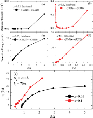
Figure 4. (a) Intraband ( ) oscillator strength for
  and (b)
  as a function of the dimensionless parameter
  . (c) Intraband (
 ) transition energy for
  , and (d)
  as a function of
  . (d) Efficiency η as a function of
  for
for  and
and  . In all cases, the structural parameters are
  , and
, and  . The solid lines are guides for the eyes.
Download figure:
Standard image High-resolution imageThe behavior of the intraband oscillator strength indicates large efficiency values for small separations ( ). This is seen in figure 5, where the dependence of the QD-IBSC efficiency η, with the interdot separation d, is depicted for optimum R values. For small interdot separation (
 ), the efficiency η reaches large values from 20%–26% for concentration in the interval
  . As x increases, the efficiencies become smaller, reaching values of the order of 1%–3%. Furthermore, it is possible to establish a connection between the efficiency and the optical oscillator strength. In particular, for
  and
and  , we notice that
  is significantly larger than
  . This may lead us to conclude that it is necessary to keep the IB evenly populated, despite the low efficiency mechanism that transfers this population to the extended state. However, there is an optimum optical transfer between the intermediate and extended levels for
  , where
  and
and  are comparable, shown as red dots in figures 3(c) and (d).
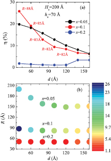
Figure 5. Maximum efficiency η as a function of interdot separation, d, for selected QD radii and different values of Mn concentration, x. In (a), each point represents the efficiency calculated for a single optimum R value. The red numbers near the efficiency values for  correspond to the R values that maximize efficiency. Panel (b) shows, in color scale, the efficiency as a function of distance and optimum radii values. Also, the bubble diameters are proportional to the calculated efficiency. In all cases, the structural parameters are
  , and
, and  . The solid lines are guides for the eyes.
Download figure:
Standard image High-resolution imageFor large separations, η decays sharply until near zero values for all considered concentrations. In the regime  , the efficiencies are less than 5%. For even longer separations, the system behaves as two independent QDs and the efficiency becomes near 1%. Thus, we can conclude that well engineered coupled nanostructures as double QDs are promising candidates to attain large efficiencies in QD-IBSC.
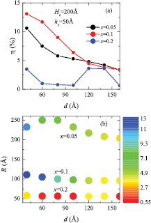
We are going to examine whether these conclusions remain valid when we decrease the QD height hz. In figure 6, we show the efficiency for  , keeping the same sample size
  . In overall form, the dependence of the efficiencies with interdot distance are very similar to those shown in figure 5. We found a significant difference when comparing the behavior of efficiency in terms of QD height d: whereas in figure 5 (
 ) the maximum efficiency obtained is
  = 26%, in figure 6 (
 ), the maximum efficiency obtained is
  = 13%. This behavior is expected since a decrease in QD height is equivalent to a reduction of spatial confinement, which causes an increase in the energy of the intermediate level (bound to QD). Therefore, the energy of intraband transition decreases, which leads to a significant reduction of efficiency, as discussed in the context of figure 4.
Figure 6. Same as in figure 5 for the structural parameters:  , and
, and  . The solid lines are guides for the eyes.
Download figure:
Standard image High-resolution image
In table 1, we collect the maximum values of efficiency for given concentrations, x, and QD heights hz. Asterisks mark the largest efficiency values,  , for a specific choice of x and hz. It is important to note the range of maximum efficiency obtained,
  %–32%. These results reinforce the clear possibility to use systems based on multiple QDs as solar cell hardware. However, the structural design of the QD system must be extremely careful in order to emulate the conditions of the present calculation. By examining the largest efficiencies
  for a given concentration x, we realize that they occur following a direct relation between
  ratio and QD height hz. We found an approximately linear relationship between hz and
  of form
  , that defines a path where we find the best values of efficiency
  for a given x. Obviously, this relationship depends on the choice of materials and the structural parameters of the sample. For the particular case of
  , we found
  , and
, and  . Finally, we found that even for large Mn doping (
 ), it is possible to obtain appreciable efficiency values, as can be shown in table 1 for QD height
  . This behavior demonstrates the flexibility of the QD system and materials as a potential IBSC device.
Table 1. Maximum efficiencies  for a DQM-IBSC with given values of x and hz. The pair the numbers in parenthesis are the optimal values of R and the ratio
  . The largest values of
  for given x and hz are marked with asterisks. In all cases
  .
.
hz( ) ) |
x | Maximum efficiency  (%) (%) |
|---|---|---|
| 50 | 0.05 | 10.6 ( , ,  ) ) |
| 0.1 | 13.1* (111, 2.775) | |
| 0.2 | 3.5 (58.1, 1.42) | |
| 70 | 0.05 | 19.8 (200, 5) |
| 0.1 | 25.8 * (87.7, 2.19) | |
| 0.2 | 1.8 (51.3, 1.28) | |
| 90 | 0.05 | 32* (143, 3.5) |
| 0.1 | 13.5 (77, 1.925) | |
| 0.2 | 14.4 (47.8, 0.39) | |
4. Conclusions
In conclusion, we theoretically study the potential application of Mn-doped II-VI CdTe/CdMnTe coupled QDs as IBSC hardware. By means of the multiband  method, we systematically explore the different QDM structural parameters as well as Mn-concentration in order to obtain optimized IBSC efficiency. Our modeling evidences the role of the intraband and interband oscillator strengths as the main ingredients to achieve large efficiencies. Our results propose a relationship between the oscillator strengths that in principle allowed us to obtain efficiencies of ≈30%. We verify that the device efficiency depends on the behavior of the intraband oscillator strengths and the intraband transition energies with the ratio
  . Thus, when both the oscillator strength and transition energy increase, the efficiency increases. The efficiency η does not increase indefinitely, but reaches a saturation value for a sufficiently large ratio
  . Finally, our numerical analysis shows that it is possible to obtain large efficiencies within a very restricted set of parameters
  whose correct determination is essential for the implementation of IBSC based on double semiconductor QDMs.
Acknowledgments
The authors gratefully acknowledge financial support from Brazilian agencies FAPEMIG: Fundação de Amparo à Pesquisa do Estado de Minas Gerais; FAPESP: Fundação de Amparo à Pesquisa do Estado de São Paulo; CNPq: Conselho Nacional de Desenvolvimento Científico e Tecnológico; Capes: Coordenação de Aperfeiçoamento de Pessoal de Nível Superior.