
Abstract
This study explores the potential of implementing the focusing properties of a virtual ideal Veselago lens within a standard free-space microwave imaging scenario. To achieve this, the virtual lens is introduced as an inhomogeneous numerical background for the inverse source problem. This numerical Vesealgo lens is incorporated into the incident and scattered field decomposition, resulting in a new data equation that involves the Veselago lens Green's function. In addition to the contrast sources within the object-of-interest, the lens introduces virtual contrast sources along the lens boundaries that depend on the total tangential magnetic field. It is shown that a surface integral contribution that takes into account these surface contrast sources must be added to the collected free-space data before one can invert using the well-conditioned Veselago lens inversion operator. A preliminary investigation of the accuracy to which this surface integral contribution must be computed is performed using additive Gaussian noise. Results show that an error of less than one percent is required to achieve imaging performance similar to utilizing an actual Veselago lens. All results are performed within a 2D simulation environment.
Export citation and abstract BibTeX RIS

Original content from this work may be used under the terms of the Creative Commons Attribution 4.0 license. Any further distribution of this work must maintain attribution to the author(s) and the title of the work, journal citation and DOI.
1. Introduction
Microwave imaging (MWI) is a non-destructive technique that uses electromagnetic (EM) radiation to determine the interior physical characteristics of an object-of-interest (OI). Over the past few decades, MWI has found numerous applications in various fields, including medical and biomedical imaging [1–3]. In biomedical applications, the interest in MWI as a possible replacement or supplementation of MRI and x-ray modalities stems from the potential to create a low-cost modality that uses non-ionizing radiation [1, 4–17]. However, as a wavefield imaging technique where the wavelength is comparable to the size of the features being imaged, quantitative MWI algorithms suffer from lower resolution. On the other hand, the specificity of MWI, due to its quantitative nature is a desired feature. Thus, any improvements to increasing the resolution would move the technology forward, closer to being accepted as a clinical imaging modality.
The inverse scattering problem (ISTP) associated with MWI is inherently nonlinear and ill-posed, allowing only a limited amount of information to be extracted from the measurement data. It does not have a unique solution and is sensitive to small perturbations in the collected measurement data. The ill-posedness of the ISTP originates in the associated inverse source problem (ISP) which is a linearization of the ISTP in terms of contrast sources. Focusing on the ISP allows one to concentrate the effort on the underlying ill-posedness. Of course, many advanced regularization techniques have been developed during the past decades, usually embedded in the iterative algorithms used for the ISTP. Actually, the multi-illumination scenarios utilized in a typical ISTP are indeed a form of regularization, wherein, although the contrast sources change with the illumination, the contrast of the OI remains constant. Therefore, implementing various additional forms of regularization in solving the ISTP has been a means of obtaining reliable imaging results. On the other hand, if one could achieve improved recovery of the contrast sources, for a single illuminating source, the impact would indeed be great.
In the last two decades, following Veselago's seminal work on the focusing phenomenon of double-negative materials [18], numerous researchers have undertaken investigations into the properties of these materials for various applications [19], including MWI [20–24]. The utilization of an ideal Veselago lens (VL), a loss-less double-negative material with  , in quantitative MWI, has been successfully demonstrated in previous research [25].
Despite the demonstrated potential usefulness of ideal VLs in various applications, such as MWI, their practical implementation has been hindered by the absence of a natural material with the required properties and the associated technical challenges of fabrication. Nonetheless, recent investigations have revealed that the use of a VL can significantly mitigate the ill-posedness of the inverse source and scattering problems associated with MWI, as reported in [25]. This is accomplished because the VL Green's function (GF), previously derived in closed form in [26], produces a well-conditioned matrix in the discretized ISP. It was shown in [25] that the quality of the inversion results was limited only by the signal-to-noise ratio of the collected data.
In this research, motivated by the unique properties of the VL, we propose a theoretical and numerical study of a non-physical VL, achieved by considering an inhomogeneous background possessing a double-negative profile. Our goal is to evaluate the potential of exploiting the lens's focusing properties without physically realizing it. To achieve this objective, we consider an imaging scenario in which the VL is absent in the total field measurement process. The problem is then split into the incident and scattered-field problems in the presence of the VL inhomogeneous background. It is noteworthy that in the standard approach of considering an inhomogeneous background in MWI, the contrast outside of the imaging domain is zero. However, it will be shown that unlike the inhomogeneous background used in the conventional imaging set-up, the inhomogeneous background which functions as a virtual VL (VVL) here, is defined outside of the imaging domain.
Subsequently, we employ the concept of the distributional derivative to state the ISP based on the contrast generated by the VL boundaries. Then, we revise the data equation presented in [25], which was introduced for the case where an actual physical lens was utilized. This revision involves the inclusion of two improper surface integrals along the VL boundaries (line integrals in the 2D problem considered herein), and the accuracy of the ISP solution relies on the precise calculation of these integrals. The surface integrals represent the add-on data in the VVL ISP and their value must be evaluated and added to the VL data. If it is possible to evaluate the surface-integral contribution the corrected data could then be directly inverted using the VL Green's operator proposed in [25], with the analytic kernel for the VL GF described in [26].
However, accurately computing the surface integral contribution is a challenge, as it requires the tangential magnetic field along the VVL boundaries. As will be shown, the true value of the surface integral contribution to the data can be obtained by comparing the VVL problem to both the VL problem and the standard MWI problem in the free space. Numerical results are obtained by inverting synthetic data created by assuming the true contribution of the surface integral and corrupting it with Gaussian noise. Preliminary results show that corrupting the true add-on data with an error of less than one percent, results in new VVL data that are invertible producing high-accuracy imaging.
The paper is organized as follows. Section 2 defines the ideal VL using step functions to represent double-negative properties of the VL. A new 2D internal boundary value problem (BVP), using distributional derivatives, is formulated for the VL. Additionally, the concept of virtualizing the VL is introduced where BVPs for the VVL scattered and incident fields are defined.
In section 3 details of using the VVL in a free-space MWI scenario are provided. Two mathematical formulations of the ISP are given: using either the traditional method of dividing the problem into three separate regions or using the distributional derivative approach. In the latter approach, it is shown how the VVL boundary conditions are converted to a single inhomogeneous Helmholtz partial differential equation (PDE) for the scattered fields applicable over all regions. The inhomogeneity consists of two surface distributions occurring at the VVL boundaries.
Section 4 derives the VVL data-equation utilizing the inhomogeneous Helmholtz PDE. The result is the same data-equation as for imaging with an actual VL [25], plus the addition of two line integrals arising from the virtualization procedure. These line integrals represent what we refer to as add-on data that must be added to the collected free-space data so as to properly perform inversion. The section presents the ISTP of the VVL in matrix form, accompanied by an explicit representation of the line integrals for direct computer implementation.
In section 5 we provide estimates of the tolerable error for computing the add-on data. Synthetic imaging results when the add-on data is computed with different amounts of error are provided. Finally, section 6 presents some concluding remarks summarizing the findings discussed throughout the paper. Details of all the mathematical derivations are given in the appendices.
2. Virtualization of an ideal VL for ISTP implementation
2.1. Mathematical formulation of an ideal VL
We consider the VL to be an infinite slab of permittivity  and permeability
  situated in free space and located between the surfaces
  and
and  . The width is denoted by
  . The surfaces of the VL will be denoted as

where Si is defined by

for  . As we will only consider line-source excitations we can limit ourselves to the 2D xy-plane for the description of the geometry and the fields associated with such a source.
To easily manipulate the physical parameters of the VL we introduce the VL step-function

where

so that the permittivity and permeability functions become

respectively, for any position  in any of the three regions
  ,
,  , and
, and  , created by the VL and identified as I, II, and II and, respectively, in figure 1.

Figure 1. VL can focus waves by negative refraction [18]. The VL problem domain is split into three main regions I, II, and III depending on the physical index of the background.
Download figure:
Standard image High-resolution imageFor the 2D time-harmonic EM problems considered herein, we assume an  time-dependence, where
  and ω denotes the radial frequency. The time-dependence is not shown in the subsequent discussions.
We assume that an illuminating z-directed line-source is located within the problem domain, V, at  in front of the VL having current density of magnitude I and defined by

where  denotes the unit vector in the z-direction and
  is the Dirac delta function. This current-source will produce only a 2D TMz
polarized field having components Ez
, Hx
, and Hy
. These satisfy Maxwell equations and can be concisely written, using the previously defined VL step function, as
is the Dirac delta function. This current-source will produce only a 2D TMz
polarized field having components Ez
, Hx
, and Hy
. These satisfy Maxwell equations and can be concisely written, using the previously defined VL step function, as


It is typical to solve these first-order PDEs by converting them to a second-order Helmholtz equation for any of the field components. But, having introduced the VL step-functions this would necessitate taking derivatives across the discontinuity. Thus, the traditional approach is to deal with the three regions separately and 'stitch' the solutions in each region together using the boundary conditions (BCs). As we assume that no surface currents are created at the boundaries of the VL, and therefore the tangential components of the electric and magnetic fields are continuous across the VL surfaces:  , and
, and  , where
  , and the superscripts − and + represent the negative and positive sides of the surfaces, respectively.
Proceeding in the traditional approach, and treating the three regions as separate, identical homogeneous Helmholtz equations can be written for the electric field in each of the three regions, except for in Region I, where the right-hand side (RHS) of the equation becomes non-homogeneous due to the existence of the point source. Thus, we obtain the following equations:

where  denotes the Laplacian operator and k0 is the free-space wavenumber [26].
One might ask, how are the physical properties of the VL manifest in the mathematical formulation when the PDEs of the formulation are identical in each of the three regions? Clearly, it is the BCs that couple the solutions of these three PDEs and determine the final form of the solution. In terms of the electric field u, the BCs are written as

An alternate approach, employing the concept of distributional derivative, the three-region internal BVP can be equivalently expressed as an inhomogeneous Helmholtz equation given by

where  . This equation is derived in [27] (forthcoming), as well as in appendix B.2. Note that the RHS of this equation depends on Ez
, which is the unknown variable within the equation itself. Thus, if the free-space GF is used this becomes an integral equation for Ez
. On the other hand, if the second term on the RHS is considered to be part of the PDE operator, this distributional PDE is equivalent to the three-region internal BVP that represents the VL. As such, to invert this equation we require the VL GF.
. This equation is derived in [27] (forthcoming), as well as in appendix B.2. Note that the RHS of this equation depends on Ez
, which is the unknown variable within the equation itself. Thus, if the free-space GF is used this becomes an integral equation for Ez
. On the other hand, if the second term on the RHS is considered to be part of the PDE operator, this distributional PDE is equivalent to the three-region internal BVP that represents the VL. As such, to invert this equation we require the VL GF.
In [26], the closed-form solution for the VL in the presence of a line source located at  was obtained. Defining the electric field in the presence of a VL in terms of the GF for the VL,

then  satisfies the following BVP:


Note the change in signs in these BCs compared to those for the electric field in (8). The VL GF was shown to be
where  denotes the Hankel function of the first kind of zeroth order,
  ,
,  ,
,  ,
,  , and
, and  . This 'Green's function' is valid for
  . Note that the coordinates
  and
and  are the locations of the singularities produced by the ideal VL, and they both depend on the location of the point source,
  .
.
The physical interpretation of (13) has been described extensively in [26], but here we provide a brief summary of the remarkable features of the VL and how they are exemplified by (13). The free-space GF for a 2D point source is given by the second-kind Hankel function,  , centered at the location of the applied source, where
  is used because to the left of the lens we are in free space and we are assuming the
  time convention. The first boundary of the VL,
  , transfers all spectral content reaching that boundary into the interior of the lens [19]. Thus, at
  the BCs given by (12) dictate that the field also be of the form
  , representing the field of a point sink located at
  . That this is a sink of energy comes from the fact that we are forced to use a second-kind Hankel function,
  , to satisfy the BCs in this first interior region,
  , but now we are in the double-negative medium of the VL. Although the phase of
  propagates outward from the sink location,
  , the power flows towards
  , as can be confirmed via the Poynting vector. Once we reach, what we refer to as, the power transfer plane,
  , all the spectral content of the energy must continue to flow to the right from the sink which forces us to use the first-kind Hankel function
  . In the double negative medium
  has the properties of outward flowing power but inward phase velocity. Therefore, in both of the interior regions,
  and
and  , we have backward traveling waves with respect to the phase velocity but the power consistently flows to the right. The boundary condition at
  dictates that we continue to use
  to the right of the lens boundary until we encounter another singularity at
  . The region
  is free space so
  represents an incoming wave towards the singularity at
  , a sink of energy. At the power transfer plane located at
  , again the power must pass through to the right,
  , so we utilize
  . We refer to the two virtual singularities created by the lens, one interior to the lens at
  and one exterior to the lens at
  , as power-transfer singularities because they are both sinks and sources of power.
In what follows, we require the GF for the case where the source is situated at the boundaries of the VL. These two cases can be simply found by consistently imposing the focusing behavior of the VL when a source is located at either boundary.
Case I: as shown in figure 2(a), when the source is located on the first VL boundary,  , the VL merges the source's location with the internal focus point and moves the external focus point to a distance of 2d to the right of the VL. Therefore, observing from a point,
  , located in Region III, i.e when
  , we can write

where  .
.

Figure 2. A schematic of the special cases of the VL field due to a point source. (a) Case I: the point source is located on the first VL boundary at  . (b) Case II: the point source is located on the second boundary at
  .
.
Download figure:
Standard image High-resolution imageCase II: as shown in figure 2(b), when the source is situated on the second VL boundary at  , this corresponds to a horizontal reflection of Case I because we can think of this case as where the first boundary of the VL is now located at
  . Consequently, the two focus points are generated on the opposite side of the VL compared to Case I, specifically on the left side. Therefore, observing from a point,
  , in Region III, i.e when
  we can write

where  .
.
2.2. Virtualizing the VL for use in the ISTP
Before we introduce the concept of a VVL, it is useful to review the general concept of using a numerical inhomogeneous background within a typical ISTP. Consider the conventional ISTP where an OI is positioned within a well-defined imaging domain, D. Assume that the OI is immersed in free space. The OI is nonmagnetic but has complex permittivity  , thus we define the relative permittivity for the problem within the problem domain V as

The total field  , which is the field in the presence of the OI as well as the illuminating source,
  , satisfies the inhomogeneous Helmholtz equation

where  is the wavenumber.
The methodology of using a virtual inhomogeneous background employs a numerical background medium with relative permittivity defined by  , for both the incident and scattered-field problems [28–33]. Hence, the incident field
  is defined to satisfy the following Helmholtz equation

where  is the non-constant wavenumber.
Then, using the definition for the scattered field,

we obtain the following Helmholtz equation

In this equation, we define the contrast source by

and the contrast function as
Note that introducing the virtual background is a purely numerical strategy to aid in the ISTP. In the past, the permittivity of the virtual background,  b
, has been chosen to be different than the true physical background, in this case,
b
, has been chosen to be different than the true physical background, in this case,  , only within the imaging domain D. The effect of introducing such a numerical background is two-fold. Firstly, it changes the unknown contrast that is to be found, and, via the contrast, the contrast source as well. Secondly, it modifies the solution of the BVP for the scattered field (via changing the GF for that BVP). Of course, the introduction of a virtual background also requires that one calculate the incident field for that background, i.e. the incident field at the receiver points cannot be physically measured.
The remaining steps of the ISTP stay the same. Several illuminating sources can be used, each of which produces a different total field that modifies the contrast sources. The contrast, on the other hand, remains the same for each illuminating source. Note that when using the virtual background in a practical MWI problem one measures the total field and computes the incident field at the receiver points to obtain the scattered field for the employed inhomogeneous background. The virtual inhomogeneous background medium approach has been used successfully for MWI in various applications [28–33], prompting the inquiry into whether such a technique can be used to virtualize the VL, i.e. without the necessity of creating double negative materials for practical implementation.
The first attempt at creating a VVL might be to simply replace the inhomogeneous background permittivity with that of the VL. That is, to simply set  and use the Helmholtz equation for the scattered field defined by (20). In this case, the wavenumber of the inhomogeneous background for the VVL is equal to the wavenumber of free space throughout the entire problem domain. That is,
  everywhere but this would completely ignore the effect of the lens's BCs.
We will see that BCs (8) obtained for the VL problem will also apply to the VVL incident-field problem. On the other hand, it will be shown that BCs for the scattered-field problem associated with the VVL will require an inhomogeneous RHS due to an induced surface contrast source at the VVL boundaries. This induced surface contrast source depends on the total field along the boundaries of the VVL. More specifically, this inhomogeneous term is proportional to the tangential component of the magnetic field along the boundaries. The magnetic field, of course, is obtained in free space and depends on the OI. The precise mathematical formulation and algorithmic MWI procedure required to implement such a VVL is described in the next section.
3. Formulation of the ISTP for the VVL
3.1. MWI setup using a VVL
Schematics of the MWI procedure employing a VVL are depicted in figure 3. Figure 3(a) depicts the total-field problem. The OI is placed within the imaging domain, D, and is illuminated by a source, S located at  creating the total field. The background properties are those of free space (i.e. no lens is present). The imaging domain D contains an object of unknown permittivity
  . The problem domain V is all of the free space. The total field is measured outside the imaging domain at various locations within the measurement domain DR
, which is a 2d-translation of D to the right of the imaging domain. The discretization of D is also 2d-translated and used to discretize DR
. Specifically, each vertical column of cells labeled as
. The problem domain V is all of the free space. The total field is measured outside the imaging domain at various locations within the measurement domain DR
, which is a 2d-translation of D to the right of the imaging domain. The discretization of D is also 2d-translated and used to discretize DR
. Specifically, each vertical column of cells labeled as  within the imaging domain, D, corresponds to a column of receivers labeled as
  , located 2d away to the right of D. In other words, corresponding to the ith
column of cells of the discretized OI located a distance li
from the VL, there will be a column of receivers on the other side of the VL located a distance of
, located 2d away to the right of D. In other words, corresponding to the ith
column of cells of the discretized OI located a distance li
from the VL, there will be a column of receivers on the other side of the VL located a distance of  from the VL.
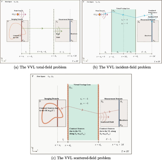
Figure 3. A schematic of MWI using a VVL. (a) The VVL total-field problem is assumed to be similar to that of the conventional MWI problem, that is, without the VL. (b) The VL is viewed as an inhomogeneous numerical background with a double-negative profile in the incident-field problem. (c) The scattered field is obtained by subtracting the incident field from the total field using equation (19).
Download figure:
Standard image High-resolution imageHence, this phase of MWI utilizing the VVL is analogous to the total-field problem in a conventional MWI technique, except for the fact that an equal number of receiver points as the cells inside the discretized imaging domain are used, and the placement of the receiver points is not arbitrary but is chosen to correspond to the original discretization inside D. This location of the receivers is similar to the demonstration of MWI in the presence of a VL described in [25], but it is important to note that this problem differs from the MWI procedure presented therein because in that work all MWI steps are conducted in the presence of the VL. Thus, to be implemented an actual VL would be required.
In figure 3(b), the virtual incident-field problem is depicted. A VVL of thickness d is now placed as shown labeled as region  ). The OI is removed but the point source is placed at the same location as when illuminating the OI in the total-field problem. The GF for the illuminating point source is used to calculate the incident field at each receiver point in the measurement domain. Notice that the VL GF is equivalent to introducing a translated illuminating point source at the location shown in the figure.
Once the incident field is computed, the scattered field is obtained by simply subtracting the numerically generated incident field from the total field measurements at the receiver points. The scattered field at the receiver points becomes the data that needs to be inverted by the new ISTP inversion algorithm. To understand the basis of that algorithm we must first consider the BVP that the scattered field satisfies.
3.2. Formulation of the BVP of the VVL
The full derivation of the scattered field BVP is provided in appendix

Subject to the inhomogenous BCs

for every  , where the contrast source is given by

and the contrast of the OI defined as

with

As can be seen from the resulting BVP, the inhomogeneous BCs reveal that when the VVL is treated as an inhomogeneous numerical background, while the field remains continuous across the boundaries, a contrast is induced along the VL boundaries at S1 and S2, which manifests as an in-homogeneity in the second BC of the scattered field.
Solving the above BVP is a much simpler task if it is converted to a single PDE in the distributional sense that is valid over the whole domain V, as was done for the GF of the VL (9), reproduced as in [27] (forthcoming). The full mathematical derivations are also provided in appendix
The Helmholtz equation for the total field corresponding to the 2D TMz free-space problem, which forms the first step of the VVL MWI setup, can be written as

where, as before,  takes care of the OI's permittivity.
The VVL incident-field problem, written in terms of the distributional Helmholtz equation of a VL (9), for  , can be written as

Thus, the scattered-field distributional Helmholtz equation can be written as

or as

with  defined as in (25). Formulating the integral equation solution to this PDE and how it can be used in the ISTP for MWI is described in the next section.
4. The ISTP of The VVL
4.1. A closed-form VVL data-equation
The VVL MWI workflow is similar to the standard approach of solving the ISTP of MWI. First, measurements of the total field, produced by illuminating the OI located in free space, are made at the receiver locations. The incident field is then computed at these same receiver locations for the same illuminating source in the presence of the VVL. The scattered field, which is the 'data' to be inverted, is then obtained by subtracting the computed incident field from the measured total field. The data-operator, which maps the unknown contrast sources inside the OI to the measured data is then inverted to obtain the contrast sources. We will focus on the ISP because it is the ISP that is ill-posed and must be solved as part of the ISTP. The unknown contrast of the OI, eventually, can be found using the obtained contrast sources and the knowledge of the total field inside the OI.
In [25], the ISP associated with performing MWI in the presence of a VL was derived and a new data-operator was introduced. The new data-equation integral operator was denoted as  , which included the VL GF, introduced in [26], as the kernel (the VL GF was herein provided in (13)). It was shown there that the discretized version of
  was well-conditioned. However, the data-equation operator for the VVL problem derived herein turns out to be different than that introduced in [26] for MWI with an actual VL as will now be described.
The VVL data-equation operator is obtained by solving the VVL PDE (31). Note that the RHS contains the incident field along the VL boundaries, whereas the scattered field is the unknown within the Helmholtz operator. Therefore, inverting this equation in the form of a data operator would utilize the free-space GF as its kernel. The goal is to create a data operator that utilizes the VL GF as its kernel so as to take advantage of the discretized version of  . To do this, we introduce the scattered field on the RHS by rewriting the incident field in terms of the total/scattered field decomposition of (19). The result is the following distributional PDE

The above Helmholtz equation with a source term due to a point source instead of the terms inside the bracket on the RHS is equivalent to the Helmholtz equation obtained in (9). This equation is equivalent to the Helmholtz equation obtained and solved separately inside the three regions of the VL problem. The solution of such a Helmholtz equation is the VL GF,  , which was introduced in [26] and presented here in (13). Therefore, to write a solution to (32) in terms of an integral equation we need to use the VL GF as its kernel.
Therefore, the solution of PDE (32) derived for the VVL problem in (23) and (24), can be finally obtained by

where  . Employing the sifting property of the surface delta distribution leads to surface integrals on the RHS as
which using Faraday's law can be written equivalently as
Note that the VL GF involved in the surface integrals in (35) can be obtained by the special cases presented in equations (14) and (15) in section 2.1. The first term on the RHS of this data equation is equivalent to the  operator in [25] which produces a well-conditioned discretization matrix. The last two terms are novel terms that involve line integrals of the free-space tangential magnetic field, or equivalently, normal derivatives of the total tangential electric field, taken over the VVL boundaries. These line-integral contributions are the 'add-on data' that needs to be added to the collected data, in free space, before we can take advantage of the
  operator.
We now turn to an analysis of this add-on data and first write the VVL data equation in a more concise form as

where

indicates the line-integrals over  . These are the improper integrals
and
Note that considering the 2D problem, both of the above surface integrals become line integrals along the boundaries of the VL. Also, note that both line integrals are improper due to the infinite boundaries of the lens.
The data that is collected in the VVL scenario is the total field collected at the receiver points, located at  , in the presence of the OI and the illuminating source. We denote this data as
  . Following the procedure of a numerical inhomogeneous background, we subtract the numerical incident field for the VVL, arriving at the scattered-field data for the VVL:

where  is the VVL numerical incident field. The solution to the ISTP for an OI incorporating the VVL is finally written as

where  denotes the scattered field for the VL problem as expressed in [25] and rewritten here as

The preceding equation holds considerable significance as it establishes the potential of MWI using a VVL by leveraging the solution of the ISTP of a physical VL, as exemplified in [25]. The two line-integral contributions to the data describe the discrepancy between the data obtained in the virtual and physical VL problems. The accurate evaluation of  is the sole prerequisite for performing MWI in the presence of a VVL. If the evaluation of these integrals can be performed with sufficient accuracy, this VVL MWI approach enables one to take advantage of the VL's properties without the need to build an actual physical VL.
Note that in an actual MWI VVL scenario the magnetic field along the locations of the VVL boundaries would be required. These boundaries are outside the imaging domain D and are related to the actual data in free space u0. Therefore, the magnetic field along these virtual boundaries is accessible in such an experiment. Unfortunately, the VVL boundaries are infinite in extent and it would be impossible to measure the magnetic field along the complete boundaries. So one needs to further investigate the use of (36). For real applications, research will have to be performed on different ways of approximating the infinite domain integrals using discrete measurements along a finite portion of the VVL boundaries. One possible method might be to measure the field around the OI and then perform a near-to-far field expansion to obtain the required field along the VVL boundaries. In the present 2D scenario, this would mean expanding the field along the VVL boundaries using cylindrical wave functions with coefficients derived from measurements made on a circular boundary circumscribing the OI.
Another possibility is to investigate the evaluation requirements for these surface integrals by expressing the add-on data in terms of the volumetric contrast sources due to the OI,  . We perform such an evaluation in the final section of the paper.
4.2. Explicit form of the line integrals
Assuming that we have expressions for the field along the VVL boundaries, we study the add-on data that is required for the VVL ISTP. To evaluate the surface integrals (38) and (39), one needs to find the partial derivative of the free-space total field along with the VVL's boundaries. From (19) we know that

Thus, recalling that  , we may find the partial derivative of the total field with respect to the x-component of
  , xS
as
, xS
as
Moreover, given that the source points for the VL GF involved in the surface integrals  and
and  in (38) and (39) are located on the VL boundaries, it is necessary to utilize the specialized descriptions of the VL GF, as introduced previously in (14) and (15).
Hence, in view of the receivers positioned within Region III, the VL GF that pertains to the line integrals (38) and (39) can be written

and

respectively.
Employing the descriptions (45) and (46) as well as the relations for the partial derivative of the total electric field in (44) gives rise to final explicit formulas for the line integrals  and
and  as
as
and
respectively, where C is a constant defined by  and
and  .
.
These line integrals are dependent on the OI and therefore evaluating the effectiveness of the VVL MWI procedure by replacing the add-on data with the computation of these integrals will depend on several factors. For example, because these integrals require the field from  to
to  a study is required on how far these improper integrals can be truncated while maintaining sufficient accuracy. That is, this will depend on how quickly the total field drops off along these lines, which will in turn depend on the OI. Such a study is beyond the scope of the present work, but some indication of the accuracy required can be ascertained by the observations discussed in the next section.
5. Investigation of the add-on data
5.1. Estimation of tolerable error in add-on data
Recall that the total field in the VVL problem is the free space total field of the OI illuminated by the source. To simplify notation we will denote the fields by u, e.g. the total electric field will be denoted as  . Thus,

A Similar expression, using  , represents fields obtained in the presence of an actual VL.
The data equation for the standard problem of MWI is

where  indicate the same contrast sources as defined in (25) created by the same OI as considered in figure 3. On the other hand, recall that the free space total field can be split into the VVL incident and scattered fields as in (19). Knowing this and then using the descriptions of data equations in the virtual, physical, and standard approaches introduced, respectively, in (40), (42) and (50), we obtain an alternative approach for describing the surface integral
  as
as
In this form, we clearly see that the add-on data,  , in equation (37), can also be represented as the difference between the total field at the receiver points performing the imaging in free space and the total field at the same receiver point locations measured in the presence of an actual VL. As in the expressions for
  using the line integrals that depend on the total field along the VVL boundaries (and in turn depend on the OI), it is also evident that the expression derived for
  in equation (51) is also contingent upon knowledge of the unknown contrast sources
  . Consequently, while this relationship is unsuitable for evaluating the add-on data in a practical situation because knowledge of the OI is required, it can be utilized to estimate the amount of tolerable error in the add-on data,
  .
.
To achieve this analysis, we first subtract the vector of incident field data at the receiver points in the VVL problem,  , which is the same as that in the VL problem, from the vector of total-field measurements in free space,
  , as
, as

This equation is the fundamental equation defining the collection of data in MWI using the VVL procedure.
To obtain the vector,  , we perform two separate synthetic experiments for the same OI to generate the numerical scattered-field data in free space, denoted by
  , and the numerical scattered-field data in the presence of an actual VL, denoted by
  , as described in [25]. Then, we use (51) to find a vector equation to compute the vector
  by
by

where  is the vector of the corresponding differences of the numerical incident field in both problems as described by (51).
Recall that in the VVL procedure, after one acquires  , one has to calculate
  using the line integrals of the total field, and subtract it from
  to form what would be the data in the VL scenario,
  . This is summarized in equations (41) and (42). Here, instead, we subtract a corrupted version of
  from
from  to obtain

In this formula we obtain the corrupted 

where  is the true add-on data obtained via (53), and
  is a randomly generated vector created as

where ξ is the percent error we want to corrupt the add-on data with, 1 is a vector of  s, and the random vectors
RV
are distinct uniformly distributed vectors of real numbers in the interval
s, and the random vectors
RV
are distinct uniformly distributed vectors of real numbers in the interval  , for the real and imaginary parts.
With this corrupted data, we continue with the VVL inversion procedure; this utilizes the discretized VL Green's operator,  , introduced in [25], to obtain the reconstructed contrast sources as

Numerical results for different amounts of percent error, ξ are presented in the next section.
5.2. Numerical results
All conducted experiments utilize a single monochromatic illuminating source. The dimensions are given in terms of the wavelength, λ. For all the experiments the left boundary of the domain, D, is positioned at a distance of d from the VVL. This requirement ensures that the total width of D corresponds to the width of the VL, which is the maximum distance away from the VVL where focusing will occur. For the example considered herein, a single illuminating source is located on the same side of the VVL as the OI, which is positioned at a distance of  from the VVL and one wavelength above the imaging domain.
Figure 4 shows the results for the true permittivity and reconstructed permittivity of the test target depicted in figure 4(a). It also shows reconstructions when noise according to (57) is added to the synthetic data ( and
and  ).
).
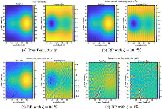
Figure 4. The true and reconstructed permittivity (RP) of the OI obtained by one illuminating source and adding corrupting noise to the synthetic data created by  , and
, and  .
.
Download figure:
Standard image High-resolution imageAs depicted in figure 4(a), the test target is comprised of two overlapping 2D Gaussian functions situated within the square  imaging domain. The imaging domain, D, is discretized into 25 cells in both the x- and y-directions, resulting in a total of 625 unknowns that are reconstructed based on 625 scattered-field measurements. Specifically, the maximum permittivity values chosen for the left and right Gaussian functions are
  and
and  respectively. The selection of this target is motivated by its characteristics: it represents a lossy target with a continuous profile, yet it contains small sub-wavelength features that pose challenges for reconstruction using most imaging techniques. In all figures presented within this paper, the color maps are carefully selected to correspond to the maximum and minimum values of the reconstructed contrast.
The matrix inversion method presented in equation (57) is first used to obtain the contrast source. Then, as in [25], the total field within D is computed and the contrast is obtained by dividing the contrast source at each pixel by the corresponding total field. The resulting permittivity is illustrated in figure 4(b). The input for this reconstruction is the corrupted measurement matrix  created using equations (55) and (56), where the percent error is specified as
  . It is important to note that this exemplary reconstruction demonstrates an excellent result achieved when, effectively, no noise is introduced into the generated synthetic data. It shows, what was demonstrated in [25], that a VL can be used to effect almost perfect quantitative imaging.
Figures 4(c) and (d) present the reconstruction for the same target, but now with increased corruption utilizing the corrupted matrix  with, respectively,
  and
and  errors, denoted as
  and
and  . As observed in the last figure, the reconstruction quality is significantly compromised. These results reflect the similar effect that adding random noise to the collected data had in [25], but there the added noise was not correlated to the add-on data,
  .
.
It was shown in [25], that to mitigate the error and enhance the recovered contrast, a possible approach is to treat the corrupted error as high-frequency spatial noise when considering the contrast as a 2D image. In this regard, two noise filtering techniques, based on truncated singular value decomposition, were introduced. These regularization techniques could also be applied here but the full study of such techniques is beyond the scope of this work. The focus of the present work is to demonstrate that the VL can be virtualized in such a way that the free-space ISP can be converted to an equivalent ISP where the data is collected in the presence of an actual VL. The reformulation of the free-space ISP using a VVL can be looked upon as a regularization technique in itself.
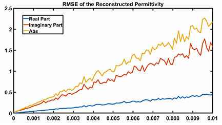
The plot of the root mean square error (RMSE) of the real, imaginary, and absolute value of the reconstructed permittivity, normalized by the maximum of the absolute value of the true permittivity of the OI over the interval, is presented in figure 5. The graph illustrates the relationship between the error and the parameter ξ, which spans the range of 10−6–10−2, corresponding to a total of 100 synthetic experiments for the same OI. It can be observed that the error approaches nearly zero when a  error is imposed. However, as the percentage of the noise in the data increases to
  , the normalized RMSE grows gradually, reaching its maximum value at 1. Starting from a negligible error near zero, the RMSE of the reconstructed permittivity starts to increase over this interval. While the real part remains always under 0.5, the imaginary and so the absolute value of the RMSE exceeds double the expected value of the true permittivity of the OI as reaching the end of the interval at
  .
.
Figure 5. The RMSE of the reconstructed permittivity normalized by the maximum value of the true permittivity as a function of percent error ξ.
Download figure:
Standard image High-resolution image
6. Conclusion
We have introduced an MWI procedure that utilizes a virtual (numerical) VL to address the ill-posedness of the associated ISP. The procedure requires only measurement data obtained as in a traditional MWI scenario, free space chosen herein, and then modifies the data equation involving the surface integrals of the tangential magnetic field along the boundaries of a VVL. The VVL boundaries are outside the imaging domain and therefore one has access to these measurements in theory, although the fact that these boundaries are infinite would require some further study to determine how far a distance along the boundaries the measurements could be truncated, while retaining satisfactory imaging results. An initial step towards ascertaining the accuracy required in obtaining this add-on data has been performed.
Future research will include the straightforward extension of the VVL concept to 3D imaging scenarios. Clearly, in the 3D imaging case the line integrals that represent the add-on data will become surface integrals. The accurate computation of these surface integrals is a topic for future study. As was briefly mentioned, a potentially fruitful way to proceed is to use near-field measurements made around the OI and then perform a near-to-far field transformation to obtain the field on the VVL surfaces.
Data availability statement
No new data were created or analysed in this study.
Appendix A: Formulation of the VVL problem. Approach 1: the three region internal BVP
This section presents the derivation of the formulation of the 2D EM field problem for the VVL illuminated by a z-directed line source. The derivation is based on a partitioning of the problem into three distinct regions, denoted as Regions I, II, and III, as illustrated in figure 1. Starting with Maxwell's equation in each of these regions a second-order partial differential equation for the electric field is derived. Thus, the permittivity and permeability of each region are considered as constants and there is no need to invoke the Veselago step functions  and
and  . The solutions in each region are coupled via BCs.
A.1. The Helmholtz equation for the VVL scattered-field problem
For the free-space problem, the three components of the total EM fields are denoted as  ,
,  , and
, and  .
.
The first-order Maxwell's equations are simply written as


where  takes care of the permittivity of the OI as in (16). As the VVL will be introduced into the incident and scattered field problems, it is useful to explicitly state that the total fields remain continuous at those boundaries:

for  .
.
As described in the main text, the incident field is defined with the same line source in the presence of a VVL. Thus, the components of the VVL incident field satisfy


Here, superscripts are used to denote the incident fields in this virtual problem. The permittivity and permeabilities, denoted by  and
and  and defined as in (4), are used to denote the material parameters in each of the three regions. The internal BCs are

for  , that is, at the boundaries of the VVL,
  and
and  .
.
Maxwell's equations for the scattered field are


subjected to the BCs

for  , where we have introduced unknown contrast sources
  ,
,  ,
,  and f that are to be determined such that the addition of the incident and scattered fields are equal to the total field.
Firstly, adding (A.2a )–(A.2c ) to (A.3a )–(A.3c ) we arrive at


Then, subtract (A.4a )–(A.4c ) from (A.1a )–(A.1c ) we find the contrast sources as

and

The contrast source f will be determined once the second-order Helmholtz equation is derived for the scattered field. We first start with solving equations (A.3b
) and (A.3c
) respectively for  and
and  to find


Then, substitute (A.8a ) and (A.8b ) into (A.3a ) to obtain

Taking the partial derivatives in (A.9), taking note that we are treating the three regions separately, we arrive at

Recalling definitions in (4), note that the wavenumber k0 is obtained everywhere both inside and outside the VL as  . So, multiplying both sides of (A.10) by
  , gives rise to

which is equivalent to

Using relations definitions (A.5)–(A.7) for  ,
,  , and
, and  in each of the different domains within V, we arrive at
Noting that there is no source inside the VL, based on (6a
) in  we have

So, equation (A.13) can be summarized into

Next, define

where  and
and  are defined as in (26) and (27), respectively. Finally, the Helmholtz equation (A.15) can be rewritten as

To determine the associated BCs and the unknown contrast function f, by virtue of the BCs, adding the BCs for the incident field to those for the scattered field BVP and then subtracting the result from the total field BCs in (A.1d ) we obtain
because the fields for the total field are continuous across the VVL surfaces. Consequently, the following BCs for the VVL's scattered-field problem are written as

Appendix B: Formulation of the VVL problem. Approach II: the distributional Helmholtz equations
B.1. Preliminaries from distributions
In this section, we use the concept of distributions from [34–37], and mostly borrow the notations from [36]. We introduce this notation for the full 3D case, denoting the EM fields as  and
and  . In a region containing no volumetric sources Maxwell's equations are written as

and

where  indicates the curl of a vector field in the sense of distribution, while
  denotes the ordinary curl where the fields are continuous. Following [36], the δS
denotes the delta surface distributions centered at any surface, S, where surface currents induce discontinuous fields. The
denotes the ordinary curl where the fields are continuous. Following [36], the δS
denotes the delta surface distributions centered at any surface, S, where surface currents induce discontinuous fields. The  denotes the increment in quantity h in the
  -direction. In our VL problem, there are no imposed surface currents, so

and

On the other hand, the discontinuous VL step-function will produce distributions on the VL surfaces, as will be shown in the next appendix where we derive the second-order equations for the fields.
B.2. Distributional Helmholtz equation for a VL
Using the VL step functions, Maxwell's curl equations in a source-free region, where neither volumetric nor surface sources exist, are written as

and

Taking the curl of both sides of (B.3a ) we obtain

Similar to (B.1b
), for  , in the distributional sense we can write

where δs
is the surface delta distribution centered at  . When using (B.5), the unit vector
  is defined as the outward normal to the lens.
Now using, (B.3b ) we arrive at

where we have used  . Due to the continuity of k0 across the VL surfaces, the second-order curl–curl equation for the electric field, (B.6) can be simply rewritten as

Note that so far our derivations are valid for any double-negative lossless lens, of any shape located in free space. In the next section, we specialize our formulation for the 2D VL problem.
B.2.1. The 2D Veselago case.
For the 2D VL, the surface of the lens is denoted by  and the surface distributions required in (B.7), δs
, is the delta surface distributions centered at
and the surface distributions required in (B.7), δs
, is the delta surface distributions centered at  and
and  . The outward unit vectors
  on S1 and S2 are therefore the unit vectors in the negative and positive x-directions, respectively.
The z-directed line source produces the 2D TMz polarization, and the curl–curl vector equation (B.7) becomes

where  . The inhomogeneous Helmholtz equation for the z-component of the electric field now becomes

where we have explicitly taken into account that the outward unit vectors at the two surfaces are in opposite directions by defining

with  and
and  denoting the delta surface distribution at
  and
and  , respectively.
The RHS of (B.9) can be rewritten in terms of the normal derivative of the electric field, either on the right or left of the surfaces

Using Maxwell's equation (B.3a
), the definition of the VL step function, and the continuity of the tangential components of the magnetic fields along  , i.e.

Note that by using these same equations, we get

which simplifies to

the same BCs when the problem is dealt with as separate regions. That is, the distributional Helmholtz equation

Replaces the formulation of the VL with point source located at  and traditional Helmholtz PDEs in each region coupled by BCs (B.14), as well as continuity of electric field on
  .
.
B.3. Helmholtz equation for VVL scattered-field problem
The Helmholtz equation for the total field corresponding to the 2D TMz free-space problem, which forms the first step of the VVL MWI setup, can be written as

where, as before,  takes care of the OI's permittivity.
The VVL incident-field problem, written in terms of the distributional Helmholtz equation for  , similar to the formulation described in the previous section, can be written as

Thus, the scattered-field distributional Helmholtz equation can be written as

or as

with  defined as in (25).