


Abstract
The dynamics of water micro-particles in air can be studied by introducing a viscous force in the equations of the motion, in addition to the weight of the particle and the buoyance force. In this work, by taking account of the buoyance force, the range of the micro-particle is calculated as a function of the angle at which it is released. An analytic-numerical procedure to find the angle giving the maximum range is indicated. The effect of a convective air flow is finally studied.
Export citation and abstract BibTeX RIS
1. Introduction
During a normal conversation we emit, depending on the phoneme we pronounce, a variable number of saliva particles at speeds of the order of some meters per second [1]. The size of these particles vary from few microns to 500 μm [2]. The speed v and the radius R = D/2 of these particles, D being their diameter, are such to give low values of the Reynolds number Re = ρvD/η, where ρ and η are the density and viscosity of air, respectively. In fact, for typical values of ρ and η and for an upper value of R = 500 μm, taking velocities up to 10 m s−1, we obtain a maximum Reynolds number of about 700, well within the laminar flow regime.
This occurrence allows application of Stokes' law to evaluate the proportionality coefficient β between the viscous force  and the velocity
  . In fact, for a sphere of radius R one finds [3] β = 6πηR. By adding the viscous force
  to the weight
  of the particle and to the buoyance force
  on it, the dynamics in air can be studied. These studies have been carried out on the past mostly in the absence of the buoyance force and in still air [4–6]. The results obtained in these conditions may be helpful when trying to detect the trajectory of a micro-particle of saliva in still air to find, for example, the safe physical distance between two persons during a pandemic event. In the presence of a convective current, however, an additional forcing term, taking account of the drag due to the moving fluid, has to be considered. Droplets generated during speech have been recognized as a mechanism responsible for the person to-person transmission of Covid-19 [1, 2]. In fact, these particles, when emitted by an infectious individual, may pose a threat of infection if they are inhaled by a susceptible one. It is therefore instructive to tackle this problem by using Newtonian mechanics. In this way students may see the usefulness of classical physics in solving real-life problems.
In the present work we first consider micro-particles emitted during a normal conversation in still air. In this case, by solving second order ordinary differential equations, the time dependence of the position of the particles and their trajectories can be found. In this way, the range of the micro-particles can be calculated for various values of the radii and of the initial velocity. The rather detailed description of this first part of the problem, including the buoyance force, can be used as a part of a lecture in an undergraduate course in physics, after having discussed kinematics and Newton's second law. In a second part of the present work we add convective air flow, simulating the effect of wind or air conditioning. The case of an aspirating flow is studied, in order to see whether this type of convective motion can prevent inhalation of these particles by another individual standing in front of the speaking person at a given distance.
In the following section we therefore illustrate the problem in still air in details. By solving the equation of motion, we derive the time dependence of the position of the particles. The range of the particle and its trajectory are found in closed form. In the third section the maximum range of the particle is derived and some didactically useful considerations are made to reduce this study to the simplest projectile motion in the absence of air friction. In the fourth section the same problem is studied under stationary air flow. Conclusions are drawn in the last section.
2. Dynamics in still air
Let us consider the motion of a spherical water micro-particle of mass m and radius R in still air under the influence of the following forces: the weight  , where ρW is the density of water, g is the acceleration due to gravity,
  , and
, and  is the unit vector in the vertical direction; the buoyancy force
  , where ρA is the density of air; the viscous force
  , where β is the friction coefficient and
  is the particle's velocity. By applying Stokes' law, we can express the coefficient β as follows: β = 6πηR, where η is the viscosity of air. We can thus write the sum of the weight and the buoyance force as follows:

Therefore, Newton's second law for the micro-particle can be written as follows:

Along the x and y directions, we write, respectively:


Equations (3a) and (3b) can be written as follows:


where  . General solutions of equations (4a) and (4b) are:


where  . Considering that the particle is emitted, at t = 0 s, from the origin of a Cartesian system of axis and setting
  and
and  , where θ is the angle the initial velocity
  makes with the x-axis, we have:


The solutions in equations (5a) and (5b) will thus attain the following form:


The terminal velocity is obtained from equations (7a) and (7b) by taking the limit for t → ∞, so that:

In order to find the time dependence of the position vector  , we write:


The definite integral appearing in equations (9a) and (9b) can be calculated as follows:

In this way, we have:


The trajectory of the particle can now be derived in closed form as follows. Let us first find the factor  and the time t from equation (11a):


where we require that x < v0 τ cos θ. By substituting the above relations in equation (11b), we find:

In the present case we do not consider large values of the quantity τ with respect to the time of flight tf of the particle which, as shown in appendix

For R = 100 μm, air at 20 °C, so that η = 17.1 × 10⁻⁶ Pa s, one has τ100 = 0.130 s. This value is still smaller for particles with smaller radii. In fact, for R = 50 μm one has  , and for R = 20 μm the characteristic time is
  .
.
3. The maximum range of the particle
In the case of the projectile motion, i.e. in the absence of viscous and buoyance forces, the problem of the optimum angle θ* and of the maximum range GM has been addressed by Lichtenberg and Wills [7]. The results found by these authors can be written in the following simple form [8]:


where v0 and vf are the initial and final speed, respectively. If the landing surface of the particle, for example, is placed at y = −h,  . At the same time, we can define the enveloping parabola which encloses all trajectories at a fixed value of v0. Therefore, a projectile, launched with initial speed v0 at an angle θ, such that
  , cannot go beyond the parabolic curve [9]:

In figure 1 this curve is represented by a dashed black line and parabolic trajectories are shown, for v0 = 4.0 m s−1 and for various angles θ. In elementary physics courses it is also shown that the various trajectories shown as coloured lines in figure 1 intersect the x-axis at x = 0 (initial position) at  [10]. In this way, the maximum value of Rθ
, which we can denote as RM, is obtained for
[10]. In this way, the maximum value of Rθ
, which we can denote as RM, is obtained for  , so that:

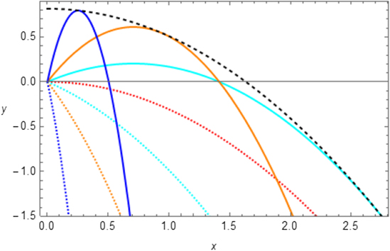
Figure 1. Parabolic trajectories of a point mass moving without friction in air for initial velocity v0 = 4.0 m s−1. The outer enveloping dashed black line is a parabola itself. For the coloured dashed curves θ < 0, for the red dashed curve θ = 0, while for full-line curves θ > 0. The following colours have been used: blue ( ), orange (
 ), cyan (
 ). Here h = 1.5 m. Axis units are meters.
Download figure:
Standard image High-resolution imageOn the other hand, if we considered a movable landing platform placed at an height H with respect to the initial position, so that  , we could argue that the intersection point between this platform, ideally described by the horizontal line y = H, and the parabola in equation (16) provides the value of the angle θ for which the farthest range is obtained for the particular value of H chosen. In this case, by taking
  , we define
  , so that equations (15a) and (15b) can be used.
While the above analysis is rather simple for the projectile motion, for the case at hand calculations are more complex. First of all, we need to adopt the correspondence  to take account of the buoyance force. Let us then denote by
  the maximum value of all the ranges
  , each calculated at a specific angle θ.
In figure 2 the trajectories expressed by equation (13) are shown for various values of the angle θ and for H = −1.5 m. Of course, these curves present different features with respect to those in figure 1 concerning projectile motion. In fact, we may notice the presence of a vertical asymptote given by the following analytic expression:

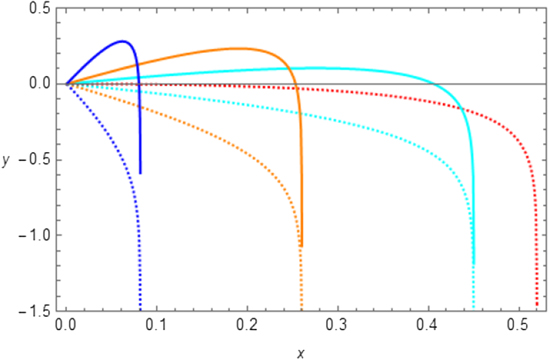
Figure 2. Trajectories of a point mass moving in the presence of air friction. For all curves the initial velocity is v0 = 4.0 m s−1, the characteristic time is τ = 0.13 s and  . The dashed red line is drawn for θ = 0, while the coloured dashed curves are drawn for θ < 0, and the full-line curves for θ > 0. The following colours have been used: blue (
 ), orange (
 ), cyan (
 ). Finally, H = −1.5 m. Axis units are meters.
Download figure:
Standard image High-resolution imageThis asymptote is the same for +θ and −θ, as it is clearly visible in figure 2, where full-line and dashed curves of the same colour are seen to coalesce as the particle approaches the landing platform at H = −1.5 m. The situation is somewhat different when the landing platform is positioned at a higher point, closer to the origin. For example, if we chose to place the landing platform at H = −0.1 m, it would not be possible to detect the asymptotic behavior of the trajectories.
Therefore, if the landing platform is positioned sufficiently below the origin, i.e. if the absolute value of H is much greater than v0 τ, all particles approach the asymptotic value given in equation (18). Therefore, in this case the θ = 0 trajectory will show maximum range and so, because of equation (18), we have:

For the specific values of v0 = 4.0 m s−1 and τ = 0.13 s, we have  , as it can be seen in figure 2. However, despite this simple way of detecting the value
  , we notice that, for H = −0.1 m, among all curves reported in figure 2, the trajectory with maximum range is the one for
  (cyan full line). Therefore, in this case the maximum range
  does not only depend on θ as in equation (18), but also on the height of the landing platform. It is interesting, for example, to consider the case H = 0. In this case we might imagine that the mouths of two closely speaking persons are at the same height. By looking at figure 2, we may see that the particles following the trajectories with θ ⩽ 0 are not able to reach the original height again, so that we might set
  for θ ⩽ 0. On the other hand,
  for θ > 0 and, among all curves reported in figure 2, the one for
  (cyan full line) shows the maximum range at
  .
.
In order to find the maximum range in these cases, we might thus adopt the following procedure. We start by setting y = H and  in the trajectory given by equation (13), so that:

By taking the differential of both sides, we have:
By now setting  , for
, for  , we get:

where θ* is the optimum angle, such that  . In this way, substituting the expression for
  of equation (22) in equation (20), we obtain:

where  . The solution of the transcendental equation (23) will provide the optimum angle θ*. After having solved for θ*, substitution of this value into equation (22) will give
  .
.
Let us then consider the solution of equation (23) for arbitrary values of the parameter a for H = 0. By setting τ = 0, 130 s,  , and v0 = 4.00 m s−1, we have
  .
.
We shall find these solutions graphically and numerically. Therefore, in figure 3 we show the graphs of the functions  and
and  in red and blue, respectively. The intersection between these two curves in the interval
  is close to
  . The value obtained by standard numerical routines is θ* = 0.4576 rad = 26.22°. With this value we can draw the trajectory having maximum range, shown in figure 4 as a black dashed line. This line shows an intersection with the x-axis at an abscissa slightly greater than the corresponding abscissa obtained by considering the cyan curve (
 ).
).
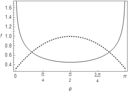
Figure 3. Graphical representation of the functions  (full line)
  (dashed line) in the interval 0 < θ < π. The solution sought is the intersection between the two curves in the interval
  , or θ = 0.4576 rad = 26.22°.
Download figure:
Standard image High-resolution image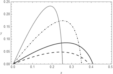
Figure 4. Trajectories of a particle released at an angle θ in air at a speed v0 = 4.0 m s−1 and for  . The characteristic time for the motion in the viscous fluid is τ = 0.13 s. The black full line represents the trajectory reaching the maximum range (θ = 0.458 rad = 26.2°). The other curves are obtained for the following values of θ:
  (dashed line),
  (dot-dashed line),
  (dotted line). The value of H is zero. Axis units are meters.
Download figure:
Standard image High-resolution imageWe have thus illustrated the procedure to follow when the maximum range cannot be found by equation (19) because the landing platform is not sufficiently below the point at which the particles are released. To resume this procedure, we may simply state that solution to equation (23) for θ* needs to be sought numerically for an arbitrary value of H. This result is successively substituted in equation (22) to find  .
.
4. Particles in a convective flow
In the previous section we have discussed the motion of a micro-particle in still air. In the present section the effect of a convective fluid flow is studied. To fix our ideas, let us assume that the fluid is stationary and that air in the vicinity of the point of release of the particle moves at a velocity  , so that we can still consider a two-dimensional motion of the particle. The viscous force is now expressed as follows
  , where
  is the particle's relative velocity with respect to the stationary fluid flow. Newton's second law for the micro-particle can now be written as follows:

Along the x and y directions, we write, respectively:


Recalling the definition of  , equations (25a) and (25b) can be written as follows:


The above equations differ from equations (4a) and (4b) by the additional constant forcing terms  and
and  in (26a) and (26b), respectively. Of course, these equations reduce exactly to equations (4a) and (4b) for vA = 0. We can therefore follow the same procedure described in section 2 to solve equations (26a) and (26b), obtaining, for the time dependence of the velocity components the following expressions:


where


are the components of the terminal velocity  , obtained from equations (25a) and (25b) by setting ax
= ay
= 0. We can now notice that the components
, obtained from equations (25a) and (25b) by setting ax
= ay
= 0. We can now notice that the components  and
and  of the velocity vector
  attain the same following formal expression, if we allow the Greek letter ξ to be x or y:

where  . By integrating at once equation (29), we obtain the following equations for the position vector components
  and
and  , both described by the quantity
  :
:

or, by substituting once ξ = x and then ξ = y:


We notice that, in the general case, it is not possible to write the equation of the trajectory in the explicit form  , as done for vA = 0, given that both equations (31a) and (31b) are transcendental. We therefore content ourselves of the parametric form of the trajectory given in equation (31a) and (31b). We can thus follow the trajectory of the particle by graphing the points
  in the x–y plane as t varies continuously from zero. Therefore, in figures 5(a) and (b) the trajectories of a micro-particle are shown for v0 = vA = 4.0 m s−1, and for the following choice of the angle θ: 0,
  ,
,  . In panel (a) the angle at which the flow is directed is
  , while in panel (b)
  . In these figures we see that the trajectories reach a maximum horizontal distance xM from the origin and then they are successively attracted back in the negative x-direction. In order to compare the effectiveness of the flow in reducing the asymptotic x-distance
  given by equation (18), in figure 6 we show the trajectories of a particle subject to a convective fluid flowing at a speed vA and released at an angle
  and
and  with v0 = 4.0 m s−1. In panel (a) the angle at which the flow is directed is
  , while in panel (b)
  . The full-line and dashed curves are drawn for a particle in still air (vA = 0.0 m s−1), the dot–dashed curves for vA = 4.0 m s−1 and
  , and the dotted curve for vA = 4.0 m s−1 and
  . One may notice that all curves obtained for vA ≠ 0 have the same inversion point with respect to the motion along the x-axis.
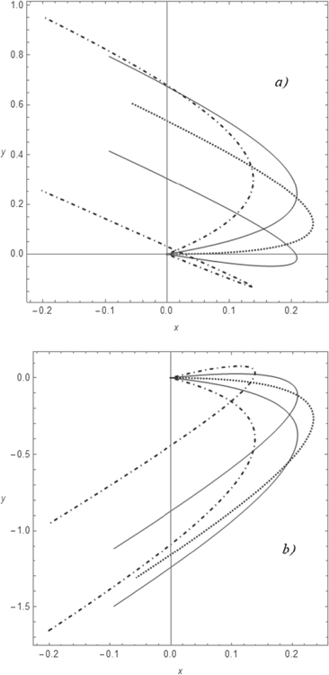
Figure 5. Trajectories of a point mass moving in the presence of air friction and a convective flow. For all curves vA = v0 = 4.0 m s−1, the characteristic time is τ = 0.13 s and  . The dotted black line is drawn for θ = 0. The upper and lower full lines are drawn for
  and
and  , respectively. The upper and lower dot–dashed lines are drawn for
  and
and  , respectively. Finally, we took
  in panel (a) and
  in panel (b). Axis units are meters.
Download figure:
Standard image High-resolution image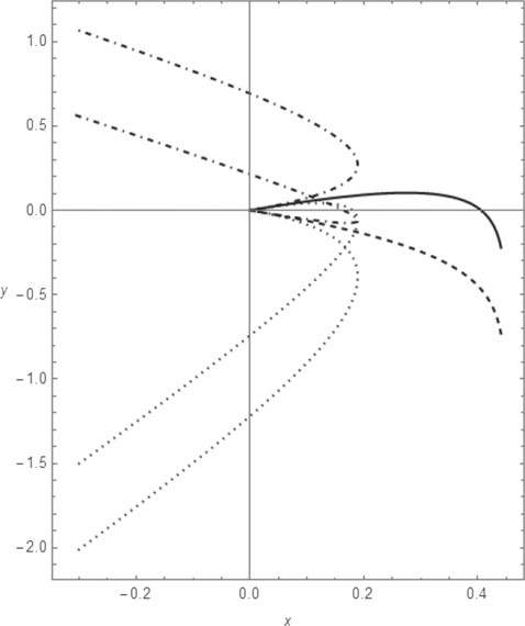
Figure 6. Trajectories of a particle subject to a convective fluid flowing at a speed vA and released at an angle θ in air with v0 = 4.0 m s−1, for  . The characteristic time for the motion in the viscous fluid is τ = 0.13 s. The full-line and dashed curves are drawn for vA = 0.0 m s−1 (still air), and for
  and
and  , respectively. The upper and lower dot–dashed curves are obtained for
  and
and  , respectively, and for vA = 4.0 m s−1 and
  . The upper and lower dotted curves are obtained for
  and
and  , respectively, and for vA = 4.0 m s−1 and
  . Axis units are meters.
Download figure:
Standard image High-resolution image
This can be understood as follows. In order to obtain the abscissa xM at which motion along the x-axis is inverted, we first need to calculate the time t* at which this inversion occurs, by setting  in equation (27a). By doing so, we get:

where we impose  . By substituting the result obtained in equation (32) in equation (31a), we obtain:

By now expressing the velocity component as v0x = v0 cos θ and vTx = vA cos α, we may write equation (33) as follows:

Being xM an even function of α and θ, we may well understand why it attains the same value for +θ and −θ at a fixed value of α, and for +α and −α at a fixed value of θ. This is also sufficient to explain why the dotted and dot–dashed curves in figure 6 present the same value of xM. Furthermore, by setting vA = v0 = 4.0 m s−1, τ = 0.13 s and by choosing  and
and  , we obtain xM = 0.19 m from equation (34). This value can well be observed in figure 6.
In order to study the asymptotic behavior of the curves in figures 5(a) and (b), we can calculate the slope mα of the asymptotic line by writing:

In this way, the asymptotic slope of all curves is independent of θ, as it could be expected.
Another feature that we notice in the asymptotic portion of the curves in figures 5(a) and (b) is the spread between the parallel asymptotes of equation  for a fixed value of α. By considering the asymptotic form of equations (31a) and (31b) we may derive the following expression for
  :
:

In this way the spread S between two curves, one at +θ, the second at −θ, for  , can be calculated as follows:

For v0 = 4.00 m s−1, τ = 0.13 s, and  , from equation (37) we have S = 0.53 m, which is the spread we measure, in figure 6, between the two dot–dashed curves and between the two dashed curves curves. The same spread could be measured if we considered convective flow directed forward at angles
  and
and  .
.
5. Conclusions
In the present work the main dynamic features of the motion of saliva micro-particles emitted from the mouth in air during a normal conversation are studied. Given the typical speeds and dimensions of these particles, low Reynolds numbers allow use of a viscous force coefficient given by Stokes' law. By considering that the effect of the buoyance force is to reduce the acceleration due to gravity, we obtained the equations of motion of the micro-particles in still air in the presence of both buoyancy and viscosity effects. From these equations the trajectory could be found in closed form. These curves present rather particular aspects as, for example, the appearance of a vertical asymptote, when the motion of the particle is not immediately stopped by a shallow landing surface. The problem of the maximum range has also been addressed. When the landing surface is placed at the same height of the point of emission of a particle of radius R = 100 μm, we find that, for an initial velocity equal to 4.00 m s−1 and for a typical value of air viscosity (η = 17.1 × 10⁻⁶ Pa s), the maximum range is obtained at angle of 26.2° and is equal to about 40.9 cm. The whole treatment can be reconducted to the case of the projectile motion in the limit of vanishing values of the buoyance force and of the friction coefficient of air.
The effect of a convective fluid flow has also been studied and some features of the model have been discussed as, for example, the asymptotic trajectories of the particles. We have notice that, for opportune choices of the convective flow velocities, the maximum abscissa reached by a particle emitted from the origin in the positive direction of the x-axis can be reduced. In this way, the convective fluid flow acts as a sucking element for the micro-particles.
The present work can be useful in determining the trajectories of saliva micro-particles emitted during a normal conversation in still air or in the presence of a convective fluid flow. Moreover, it could be a starting point to investigate further on the motion of micro-particles in air. In fact, an interesting point to be studied is the time the particles stay in air in the absence or in the presence of a convective air flow.
Basic calculus and knowledge of linear ordinary differential equations is required in this work, so that it can be addressed to first-year university students. Moreover, given the timeliness of the present analysis, the present work can be used in a lecture constructed using an inquiry based learning approach, where the engage stage can be obtained by using a sprinkle emitting tiny water particles in air.
Acknowledgments
One of the authors (RDL) would like to thank P Desideri and F Romeo for stimulating discussions.
Appendix A
We show that the expression derived in equation (13) reduces to the well-known trajectory of a projectile for negligible intensities of the buoyance and viscous forces. In this limit, from equation (12a) we may set  . By a Taylor series expansion of the logarithmic term in equation (13), we write:

where  and where only terms up to ξ2 are retained. In this way, by setting to zero the density ρA, so that
  , the trajectory can be approximated as follows:
This is the well-known expression of the trajectory of a point particle under the sole influence of its weight [10]. Alternatively, for t ≪ τ, by a Taylor series expansion of the exponential  in equations (11a) and (11b), we may set:

where only terms up to  are retained. Substituting this expression in equations (11a) and (11b) and recalling that vT → gτ, we have:

Notice that in equation (A4a) we have considered only the leading order term. Equations (A4a) and (A4b) are just the time-dependent coordinates that can be derived in the projectile motion [10, 11].
Appendix B
We here show that, for  , or a ≫ 1, solution of equation (23) gives back the results for the projectile motion of equation (15b). For this purpose, let us set y = sin θ*, so that equation (23) becomes:

Recalling the Taylor series expansion of the logarithm in equation (14) and setting  , we may write, by also taking
  :
:

By straightforward algebra, we thus have:

where, we recall,  . By the trigonometric relation
  , equation (B3) can be written as follows:

From the above equation we have  , so that equation (15a) is recovered. Equation (23), for
  , can thus be written as follows:

By using equation (15a), one can thus show that equation (B5) gives back equation (15b), proving that, for a ≫ 1, equation (23) provides the well-known results of the case of the projectile motion.