


Abstract
We analyze the problem of a quantum particle falling under the influence of a one-dimensional constant gravitational field, also known as the bouncing ball, employing a semiclassical approach for the effective equations of motion for the quantum system. In this formalism, the quantum evolution is described through a dynamical system of infinite dimensions for the position, the momentum, and all dispersions. Usually, the system is truncated to reduce it to a finite-dimensional one; however, in this case, equations of motion decouple and the system can be solved exactly. For a specific set of initial conditions, we find that the time-dependent dispersion in position follows the classical trajectory; however, for large times, it grows enough to allow a non-classical behavior for the rebounds. We also propose the study of an effective potential in terms of a pair of canonical variables for dispersions.
Export citation and abstract BibTeX RIS
1. Introduction
The descriptions of classical and quantum phenomena have in general profound differences in their mathematical formulations and physical interpretations. On the one hand, in classical mechanics, the state of a physical system is studied by analyzing its motion under the influence of external forces, where its temporal evolution is determined by a set of ordinary differential equations of motion. Once the physical variables that describe the system as a function of time have been obtained, given initial conditions, the behavior of the system at all times is known; in that sense, classical systems form a completely deterministic framework. On the other hand, quantum systems have a probabilistic description. For instance, it is not possible to know simultaneously the position and momentum of a given particle at a given time according to Heisenberg's uncertainty principle, thus the concept of trajectory is lacking. All the information about the system is encoded in the wave function  , whose squared norm gives the probability density of the system. The evolution of the wave function is determined by the well-known Schrödinger equation [1].
Given the probabilistic nature of the quantum mechanical description of physical systems, its interpretation is not always obvious since the solution of the Schrödinger equation usually requires boundary conditions even for the simplest systems. Therefore the use of approximation methods is not only desirable but necessary to study quantum systems and better understand their behavior. There exist several such methods like the well-known WKB and perturbation theory [2]. There is also the trajectory approach to quantum mechanics, which was initially developed by de Broglie and consolidated by Bohm [3]. In this formalism it is possible to obtain semiclassical trajectories from a formal definition of velocity in terms of current and probability density, v(r, t) = j(r, t)/ρ(r, t), where one first needs to solve the Schrödinger equation and then calculate the trajectories according to the previous definition.
Similarly, semiclassical approximations to quantum physics are often presented through classical equations of motion augmented by correction terms that may include new degrees of freedom associated with quantum effects. For instance, it is well known that the evolution of the expectation value of the position operator in a general quantum state is given by the Ehrenfest theorem
where the Taylor expansion has been performed to the lowest orders. This expression implies that for a sufficiently narrow wave packet the expected position follows the classical trajectory on average. However, an infinite number of corrections around such a classical path is needed to reconstruct the corresponding quantum state [4]. From the rhs of this expression, we can note that such corrections must be in terms of the quantum dispersions or higher-order moments [5]. Hence, to describe the behavior and evolution of a quantum system in terms of a set of classical differential equations, the evolution equations for quantum corrections must be included.
Based on this idea but applied to any operator, an expansion in the dispersions can be performed, from which quantum modifications are obtained systematically as deviations from the classical dynamics [6]. These quantum corrections then, come from the entanglement of quantum dispersions with classical dynamic variables. The corresponding equations for semiclassical dynamics describe the behavior of expectation values in a definite state, replacing the Schrödinger description with an infinite number of coupled equations of classical variables and quantum fluctuations. This defines an extended phase space endowed with a Poisson structure, but in this case between all classical and quantum variables. These equations are particularly useful for semiclassical states where consistent truncations can be made. The resulting expressions can shed some light on the behavior of states giving potentially observable effects. Furthermore, they naturally introduce the concept of quantum trajectory and could be important when proposing effective potentials. The essentials of this formalism can be found in the literature under different names such as Gaussian wave-packet dynamics [7, 8] or effective Gaussian dynamics [9, 10], moment equations [5], quantized Hamilton dynamics [11], and more recently, Ehrenfest dynamics, [12–14]. In the previous references they usually work in Gaussian states and do truncation only up to second order for quantum dispersions. A general method has been developed from a geometrical perspective, giving the evolution equations for dispersions to any order [6]. This method is known as effective equations of motion for quantum mechanics which we follow.
In this work we apply a semiclassical approach to a quantum particle in the presence of a gravitational potential near the surface of the Earth, also known as the quantum bouncing ball problem. It is shown that the effective approximation for this system reduces to a finite number of quantum corrections because the potential is linear in position, thus making the system exactly solvable. Although the system is rather simple, it presents an interesting behavior that can be traced at all times. This work also aims to be an introductory study for those wishing to deepen their knowledge of the effective equations method. In section 2, we review the classical and quantum dynamics of the quantum ball. In section 3, we describe the method of effective equations for the moments, analyzing the gravitational effect on the bouncing quantum ball and discuss its deviation from the classical behavior due to quantum corrections. In section 4 we discuss the obtained results in the context of the semiclassical approximation, emphasizing the use of the method of statistical moments and quantum dispersions as dynamic variables. Finally, we include appendix
2. Classical and quantum description of a particle in a gravitational potential
2.1. Experiments and applications of the quantum bouncer
A particle falling in a gravitational field is a simple long-standing problem that appears in elementary physics texts; its quantum version is an intermediate problem that has been studied in some textbooks such as [15], and in several educational papers [16, 17], due to its very interesting characteristics. Since the 1990s (see [18, 19] for further references), several experiments have been proposed due to the development of processes such as quantum cooling, manipulation of individual atoms, magnetic mirrors, and other high-precision quantum optics experiments [20–23], allowing not only the development of the quantum bouncer but also its use in many interesting models and applications.
In the past ten to twenty years, it has also attracted a lot of attention from both theoretical and experimental points of view. The experimental realization of the quantum bouncer was carried out with photons [24], and ultracold neutrons, which are very sensitive to gravitational forces and others of the same kind. By these experiments it may be possible to measure several phenomena of interest in quantum optics and these are sensitive enough to test interactions of quantum systems with the gravitational field—for example, to measure fundamental constants, to test extensions of the standard model, or gravitational problems such as the testing of the equivalence principle, non-Newtonian gravity, theories on the structure of space-time [25–28], and even to rule out dark energy models [29]. A fairly comprehensive review can be found in [30].
An interesting application of quantum bouncing is found in experiments in which Bose–Einstein condensates are dropped and it has been shown that when bouncing they exhibit a similar behavior to that of the quantum falling particle [31]. This has led to other numerical and theoretical studies where the Gross–Pitaevskii equation is solved with a gravitational potential in addition to the standard non-linear terms [32, 33].
Indeed, from a theoretical point of view, as mentioned in [15], the gravitational-type linear potential also appears when studying the energy spectrum of the quark–antiquark bond. It also may serve to provide guidance in the analysis of other types of physical systems, such as the study of lower-dimensional models of quantum gravity [34]. Even more, it has been seen that the Hamiltonian of a quantum black hole, under certain conditions, can be transformed into one with a linear potential term [35]. As we shall see, the quantum bouncer presents collapses and revivals of the wave packet, which have recently been associated with entropic information measures of how classically the system behaves [36–38].
In this section we describe the classical and quantum approaches to this problem. We will employ the classical approach by introducing our semiclassical method that considers quantum dispersions or moments as dynamic variables, while the quantized version will give us insight into how the system behaves and will serve to limit the applicability of the method.
2.2. Classical bounce
The description of the dynamics of a particle of mass m under the influence of a gravitational potential V(x) = mgx, with g denoting the gravitational acceleration, is an old well-known problem that can be studied by means of the one-dimensional Hamiltonian 4

As is well-known, for general initial conditions  , the solution of the equations of motion for the position x and momentum p as a function of time is


where g is the gravitational acceleration. Equation (2) determines the position of the particle for any time t> 0. Without any loss of generality we can choose v0 = 0; a different value of the initial velocity simply shifts the value of x0.
As in [19], we place an infinitely heavy, perfectly flat mirror at the bottom of the potential, so the system is conservative in energy and the magnitude of momentum, and we have an infinite number of parabolas, one for each bounce.
It is possible to write the general solution in such a way that bounces are noticed in the position versus time graph. The solution is then written in terms of the period T defined as twice the time needed to reach the floor,  , that is
where Θ(t) is the Heaviside step function. In certain applications, and in particular to be able to compare with the quantum result [19], it is more convenient to expand equation (4) in its corresponding Fourier series, giving the following

2.3. Quantum bounce
Now we study the quantum behavior of a massive quantum particle in the presence of this constant gravitational field. The motion of a falling particle bouncing off a mirror is known as the quantum bouncer [19, 39]; the reflective potential can be simulated by solving the Schrödinger equation in the region x> 0. For neutrons, the characteristic length scale of the system is on the pico-eVs scale, i.e. 10−12 eVs—an energy scale that can be used in measurements of fundamental constants and gravitational effects beyond Newtonian theory [28]. Possible generalizations have been studied in [40], where the mirror below oscillates and generates a chaotic system. A two-dimensional extension [41] studies a bouncer on an inclined plane. In two-dimensional cases it is interesting to study the uncertainty in the transverse coordinate. However, in the present work we will limit ourselves to the one-dimensional case.
For the gravitational potential V(x) = mgx, the quantum Hamiltonian operator is

whose eigenvalue equation is

ψn (x) are the wave eigenfunctions with boundary condition ψn (0) = 0 on the mirror below, and En are the energy eigenvalues. Equation (7) can be cast in dimensionless form by introducing a characteristic length and an energy scale


Thus, with the new variables  and
and  , equation (7) turns into an Airy equation of the form ψ''(x⋆) = (x⋆−E⋆)ψ(x⋆), whose solutions are the Airy functions Ai and Bi. Since x⋆ is not bounded, as its argument grows the function Bi also grows. So it is not a solution in this case and we consider only Ai. The boundary condition requires the wave function to be zero at x⋆ = 0, which implies that Ai(−E⋆) = 0. Thus, the solution can be written in terms of the roots xn
of the Airy function:
, equation (7) turns into an Airy equation of the form ψ''(x⋆) = (x⋆−E⋆)ψ(x⋆), whose solutions are the Airy functions Ai and Bi. Since x⋆ is not bounded, as its argument grows the function Bi also grows. So it is not a solution in this case and we consider only Ai. The boundary condition requires the wave function to be zero at x⋆ = 0, which implies that Ai(−E⋆) = 0. Thus, the solution can be written in terms of the roots xn
of the Airy function:

where the Nn are normalization constants and the Airy function Ai has the following integral representation

The energy spectrum is written in terms of the zeros of the Airy function, xn > 0, such that En = mglg xn , for n = 1, 2, ... An analytical approximation of xn for large n is given in [42], yielding for the energies

The first eigenvalue, for n = 1, from the zeros of the Airy function, is equal to E/(mglg) = 2.338 11, while the approximation (12) gives the value of E/(mglg) ≃ 2.320 25, which only differs from the former by 0.763 72%. For neutrons with mass 940 MeV/c2 the corresponding gravitational length is lg = 5.87 μm, whose corresponding energy scale is Eg = 0.602 peV, [28]. Recently, experiments showing that the transitions between the quantum states of neutrons can be triggered by the vibrations of a mirror have been proposed. In such cases the quantum bouncer is used for measurements of sensitivity in gravity tests [43, 44].
The time-dependent solution of the Schrödinger equation with Hamiltonian (6) formally is  , the coefficients Cl
being fixed by initial conditions. For a Gaussian initial wave packet
, the coefficients Cl
being fixed by initial conditions. For a Gaussian initial wave packet  , where σ is its standard deviation and x0 its peak position, in units of gravitational length, an approximation of the evolution of the expectation value for position was done [19], for high quantum energies, corresponding to the semiclassical limit.
Alm
are the matrix elements  . As shown in [19], when x0≫σ, i.e. for a localized wave-packet, the expectation value has the same periodic dependence on time as the classical one (4). This allows us to reorder and approximate the sums in such a way that, in the classical limit, the second line of the above equation is obtained, with approximation An
≃Amm+n
. Note that for large x0, the first exponential term in the sum of the last part of (13) tends to 1, and we recover the Fourier series (5) until multiplication by lg.
. As shown in [19], when x0≫σ, i.e. for a localized wave-packet, the expectation value has the same periodic dependence on time as the classical one (4). This allows us to reorder and approximate the sums in such a way that, in the classical limit, the second line of the above equation is obtained, with approximation An
≃Amm+n
. Note that for large x0, the first exponential term in the sum of the last part of (13) tends to 1, and we recover the Fourier series (5) until multiplication by lg.
As shown in [19], for certain initial states, the expectation values of the position collapse into the classical trajectory for some time, then 'revive' and start to bounce again. The revivals can be interpreted as an interference between different sections of the wave packet that have already bounced. This system has also been analyzed with the WKB approach, where the possible effect of tunneling resonances is obtained [39]. Furthermore, it has been found that a falling wave packet can have a diffractive structure depending on its initial dispersion: if it is wider than the characteristic length lg it falls as a free packet, but if it is smaller it has a diffraction pattern [45]. Certainly, the appearance of such collapses and revivals was visualized on light propagation in an optical waveguide [24]. This model has been further extended to a matter-wave soliton that bounces more like a particle compared to the wave packet [46].
3. Effective equations for the dynamics of the quantum falling particle
As is well known, it is impossible to know simultaneously the position and momentum of a quantum particle or system due to the Heisenberg uncertainty principle; that is, there exist no quantum trajectories analogous to the classical evolution. However, as we mentioned above, there is a particular semiclassical formalism in which a quantum mechanical system can be studied as a classical Hamiltonian system but in an infinite dimensional phase space, where the additional degrees of freedom are directly related to the expectation values of all the infinitely many quantum dispersions [6]. This general formalism was applied to simple models of loop quantum cosmology to show the existence of a quantum bounce at the beginning of the Universe [47–50]. However, it has also been studied in other systems such as anharmonic oscillators [51], and also two-dimensional systems such as the quantum Kepler problem [52]. This approach is also known as moment equations or momentous dynamics due to the similarity between quantum variables with statistical moments of probability distributions, although the former also contain additional quantum effects due to the non-commutativity of quantum operators [53]. An interesting feature of this formulation is that it produces a classical evolution, that is, trajectories for quantum evolution can be obtained as long as the appropriate initial conditions exist, forming an ideal ground for comparison between different approaches.
For a system with one degree of freedom, we define a set of new variables as the joint statistical moments of any order, i.e. the expectation value of powers of products of the canonical position and moment operators, as follows

where a, b are integers, and  and
and  are the expectation values of the momentum and position operators; also the completely symmetric or Weyl order of the operators is used.
The evolution of the system is generated by an effective Hamiltonian HQ, defined as the Taylor expansion around the expectation values of the canonical variables of the Hamiltonian operator; therefore the classical Hamiltonian is corrected by quantum effects due to the expectation values of dispersions, as follows
where a, b = 0, 1, 2, ..., such that a + b ⩾ 2; this last inequality is due to the fact that clearly the variables G0,1 = G1,0 = 0, from the definition. Equations of motion are obtained considering the relation

for quantum operators  , where
  . Considering that (x, p) are canonical variables, i.e.
  , then, equations of motion for classical phase variables are obtained by computing their Poisson brackets with the effective Hamiltonian HQ, equation (15)


The corresponding equations of motion for variables Ga,b
are also given by their Poisson brackets with HQ. For instance, using (14) and (16), one obtains  . Poisson brackets among moments were obtained first in [6] and extended in [54]. Although the expression is more involved, the general idea is to rewrite (14) in terms of powers of classical variables x, p and products of powers of the expectation values
  . Therefore, Ga,b
, Gc,d
reduces to computing the Poisson brackets among classical variables and the using of equation (16) repeatedly. The resulting expression is the following
. Therefore, Ga,b
, Gc,d
reduces to computing the Poisson brackets among classical variables and the using of equation (16) repeatedly. The resulting expression is the following
where the sum runs over odd numbers from  , with
 ![$1{\leqslant}\tilde {N}{< }\mathrm{min}\left[a+c,b+d,a+b,c+d\right]$](https://content.cld.iop.org/journals/0143-0807/42/1/015404/revision3/ejpabc13aieqn17.gif) , and the coefficient is
, and the coefficient is

Equations of motion for Ga,b then follow
where V(n)(x) = ∂n V/∂xn , with V being the potential of the Hamiltonian that only depends on the position operator. It was also considered that Ga,b commutes with the classical variables x and p. Furthermore, the moments Ga,b must satisfy generalized uncertainty relations, given that the square of the expectation values of the operators satisfy the Schwarz inequality [47]

where equation (16) was used on the rhs of the last inequality. Let us use this semiclassical formulation to study the quantum bouncer defined by equation (6). Generalizations to two or more dimensions are possible, however, we will not study them here as they are more involved (see for instance [52]). Therefore, for the gravitational potential V(x) = mgx we get the following quantum Hamiltonian

An interesting feature is that the Hamiltonian is finite in quantum corrections, just G0,2 appears in the previous equation, so we can obtain its exact evolution. In the case of the Hamiltonian (23) the equations of motion for expectation values x, p, reduce to the classical Hamiltonian equations because the sums in (17) and (18) do not contribute. This occurs if the effective Hamiltonian is at most quadratic in canonical variables. The equations of motion read


One can see that classical and quantum variables are completely decoupled. It is straightforward to solve them

where the classical solution for the canonical variables is the same as in (2), and c0, c1 and c2 are constants fixed by initial conditions.
We can use the solution (26) in (22) to get

Assuming that the dispersions are not initially correlated, G1,1(0) = 0 implies that c1 = 0. The inequality depends only on c0 and c2 which are the initial conditions for second-order moments. In addition, by saturating the uncertainty condition (27) we get a relation between constants fixed by initial conditions, that is

This set of initial conditions certainly are of the simplest choices one can make, however, it is possible to make an analysis for coherent dynamical states for this model, in a similar way as the Gaussian Klauder coherent states studied in [55].
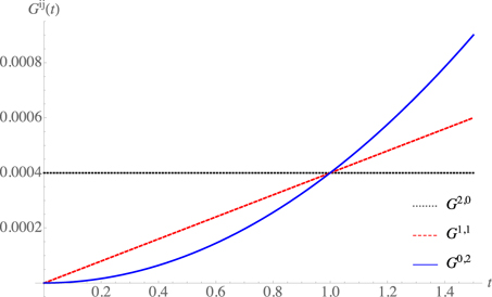
Figure 1. Behavior of dispersions of quantum variables Gi,j , for α1. Position dispersion and correlation grows over time.
Download figure:
Standard image High-resolution image
Figure 2. Semiclassical bounces for the quantum ball, and their uncertainty, x±Δx, for α1. Uncertainty grows over time around the classical solution.
Download figure:
Standard image High-resolution imageWe choose the dispersion in positions since it is the one appearing in the quantum Hamiltonian (23). Then from (28) we realize that the initial condition for G0,2(t) cannot be zero. We recall that a characteristic length exists for the gravitational field lg, as given in equation (8), and we can propose an initial condition for the moment of that order, i.e.

where α is a dimensionless constant. Using (28) we obtain  . From this we see that the solutions in (26) can be written as


The dispersion in the position is quadratic and the correlation is linear in t; that is, both grow over time, while for the momentum dispersion is constant, (figure 1). This implies that after a certain threshold time the approximation would no longer be valid. We show this behavior in figure 2.
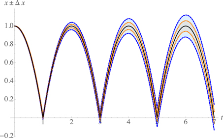
Figure 3. Trajectories with dispersion x±Δx. Solid (black) line is the classical solution, dashed (blue) line is for α1 = 1, and dotted line (orange) is for the case α2 = 4.31.
Download figure:
Standard image High-resolution imageSubstituting this last expression in (23), we can rewrite the Hamiltonian as follows

where the effective correction term for the Hamiltonian is precisely proportional to the characteristic energy of the system Eg, as given in (9). This suggests that α = 1, in such a way that the initial dispersion for the position might be the gravitational length squared. Keeping α arbitrary one gets

This Hamiltonian has a minimum non-zero energy associated with the characteristic length of the system. Indeed, it is possible to fix an alternative value for α on the basis of the energy spectrum (12), to get a lower bound for the semiclassical approximation; so one can also set α = 4.31.
The expectation value of the position approximately follows the classical trajectory (4), and around it we have the band of time-dependent uncertainty given by G0,2, as denoted in equation (29). We can express the corresponding solution with effective quantum correction as  , constrained to the initial condition v0 = 0, i.e.

It is possible to write the solution in terms of the period of the bounce as in (4), obtaining a series of semiclassical bounces bounded by the uncertainty Δx. The behavior of equation (32) is shown in figure 3 in terms of the proposed values of the dimensionless constant α. We realize that at the maximum height of the trajectory, the absolute value of the uncertainty is also maximum. Although the behavior of the dispersion is the same in each bounce, its amplitude grows with time, allowing for a more subtle evolution inside the uncertainty. The case of the momentum is very simple since the uncertainty is always constant at each point, so the graph will be a straight line with a constant fringe. Finally, the covariance is linear in t, which means that as time increases, the dispersions of classical variables will be more correlated up to a maximum in each period, due to quantum effects. Indeed the strength of the correlation is proportional to the characteristic energy Eg = mglg, of the quantum particle in a gravitational potential.
4. Discussion
We have employed the description provided by effective quantum mechanics to study the behavior of a particle under the influence of a gravitational potential. We showed how the usual Schrödinger evolution in quantum mechanics can be analyzed with an equivalent semiclassical dynamical system for which a Hamiltonian is obtained. The dynamical phase space variables of this system (x, p) together with quantum dispersions Ga,b encode all the information of the quantum system, making the study of quantum systems more tractable.
The quantum behavior of a massive particle bouncing off an infinitely heavy horizontal mirror in the presence of a gravitational field, which is usually called a quantum bouncer, is used to model some experiments to measure sensitivity in gravity tests, making it a very interesting scenario to consider. This model has also been used to test various scenarios of super symmetric gravity [56] and quantum gravity, particularly those involving specific length scales where it is possible to determine bounds for the parameters of the theory [56–59].
In this work we showed that for the case where there is no initial correlation between position and momentum, the effective Hamiltonian acquires quantum corrections related to the characteristic ground-state energy and to the gravitational length lg. We reproduce the classical trajectory bounded by the value of the time-dependent moment G0,2, which is due to the uncertainty relation. It is worth mentioning that there are previous studies in the semiclassical regime for this quantum bouncer; for instance, in [60] time-dependent solutions using different expectation values with Gaussian states were found. It is interesting to note that they obtain a result very similar to ours for the dispersions in x and p. However, since they do not consider the correlation between dispersions and expectation values, the product of ΔxΔp is a function of time, unlike our case, which is constant. In this model the semiclassical trajectory of the bouncer acquires a growing uncertainty with time, for general initial conditions and large enough time (large number of rebounds). In this way the actual behavior of the system may present a more involved evolution, for instance one can obtain a phase of decay and growth in the amplitude of the trajectory, in a similar way to the revival in [19]. The method of momentous effective quantum mechanics employed here is suitable for the quantum bouncing ball as it provides a very detailed description of the evolution of the particle, which can be contrasted with experimental observations and measurements [24, 28, 43, 44, 46]. The application of this method to the study of semiclassical states for several quantum systems, especially those for which high experimental precision is achievable, will be carried out elsewhere.
Acknowledgments
The authors want to thank the Organizer Committee of the Third Meeting of Mathematical Modeling in Physics and Geometry (Tercer Encuentro de Modelado Matemático en Física y Geometría) for the welcoming scientific environment that allowed the realization of this work. GCA wants to thank Viviana García-León for useful discussions on the subject of this paper.
Appendix A.: Effective potential and canonical variables for dispersions
We have seen the net effect that the inclusion of moments has in both the gravitational potential and the Hamiltonian (31), which is the introduction of a non-zero minimum energy. As we mentioned earlier, the quantum modified Hamiltonian HQ acquires, in general, an infinite number of momenta, even though for the present case they reduce to those of second order, that is, no truncation is needed. Although it was possible to obtain the equations of motion for moments in equation (21) from their Poisson bracket with HQ, in general, the algebra of the quantum variables Ga,b is not canonical and is somewhat involved. In a recent work though, an extension to this method was obtained where it is possible to redefine these quantum dynamical variables forming canonical pairs (σ, ρ), yielding a true canonical dynamical system [11, 61, 62]. Not just that, but under general assumptions 5 it is possible to include the whole contribution of the variables in a non-local generalized potential; a sort of quantum potential [63], allowing a richer analysis of the system.
For the second-order dispersions the canonical variables are defined as [11]

where u is a constant of motion of the system and its Poisson bracket with σ and ρ vanishes. For a one-dimensional case, the quantum Hamiltonian can be written as

where VEff(x) is the effective potential mentioned above. It reads

V(x) being the classical potential.
For our case of linear potential there is a decoupling of the equations, so the non-local term of the potential reduces to the standard potential V(x). However it is possible to write an effective potential in terms of the new canonical pair and the Casimir constant u, which can be evaluated under any initial condition. Hence, the quantum Hamiltonian is as follows

In figures A1 and A2 the behavior of this effective potential is shown. It can be seen that it flattens out as x increases, and it grows for small σ and x.
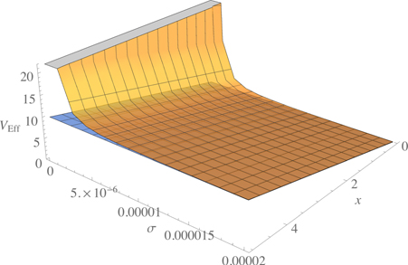
Figure A1. Effective potential as a function of configuration variables (x, σ). In blue is the plane for the gravitational potential. It is clear that the potential is greater for small σ and x close to zero.
Download figure:
Standard image High-resolution image
Figure A2. Contour plot of the effective potential. It can be seen that the effective potential is flattening with increasing x, but the effects for small σ prevail.
Download figure:
Standard image High-resolution imageFrom equation (A.4) it is possible to obtain the dynamics of the new canonical variables

whose solution is

with integration constants k1 and k2 given by initial conditions. With these new variables it is clear that an analysis with non-zero initial correlation can be performed in a straight-forward way.
Finally we plot the configuration variables, classical and quantum. In figure A3 we observe that as x decreases, σ increases; when the ball bounces, x will continue to oscillate between 0 and x0, while σ will always increase, which is consistent with the behavior described above.

Figure A3. Phase space for classical and quantum variables. While x will continue bouncing between 0 and x0, σ will always increase. Here we choose x0 = 1.
Download figure:
Standard image High-resolution image
Footnotes
- 4
It is possible to study a related two-dimensional problem where the particle bounces and advances in the transversal direction; it is also possible to include dissipation and see how the rebounds decrease in amplitude. These cases, however, will not be included in the present study.
- 5
These assumptions rest on the characteristic behavior of the dispersions and their relative hierarchy; it is found that momentum dispersions G0,b are negligible with respect to coordinate dispersions Ga,0.