
Abstract
The simplest ΛCDM model provides a good fit to a large span of cosmological data but harbors large areas of phenomenology and ignorance. With the improvement of the number and the accuracy of observations, discrepancies among key cosmological parameters of the model have emerged. The most statistically significant tension is the 4σ to 6σ disagreement between predictions of the Hubble constant, H0, made by the early time probes in concert with the 'vanilla' ΛCDM cosmological model, and a number of late time, model-independent determinations of H0 from local measurements of distances and redshifts. The high precision and consistency of the data at both ends present strong challenges to the possible solution space and demands a hypothesis with enough rigor to explain multiple observations—whether these invoke new physics, unexpected large-scale structures or multiple, unrelated errors. A thorough review of the problem including a discussion of recent Hubble constant estimates and a summary of the proposed theoretical solutions is presented here. We include more than 1000 references, indicating that the interest in this area has grown considerably just during the last few years. We classify the many proposals to resolve the tension in these categories: early dark energy, late dark energy, dark energy models with 6 degrees of freedom and their extensions, models with extra relativistic degrees of freedom, models with extra interactions, unified cosmologies, modified gravity, inflationary models, modified recombination history, physics of the critical phenomena, and alternative proposals. Some are formally successful, improving the fit to the data in light of their additional degrees of freedom, restoring agreement within 1–2σ between Planck 2018, using the cosmic microwave background power spectra data, baryon acoustic oscillations, Pantheon SN data, and R20, the latest SH0ES Team Riess, et al (2021 Astrophys. J.908 L6) measurement of the Hubble constant (H0 = 73.2 ± 1.3 km s−1 Mpc−1 at 68% confidence level). However, there are many more unsuccessful models which leave the discrepancy well above the 3σ disagreement level. In many cases, reduced tension comes not simply from a change in the value of H0 but also due to an increase in its uncertainty due to degeneracy with additional physics, complicating the picture and pointing to the need for additional probes. While no specific proposal makes a strong case for being highly likely or far better than all others, solutions involving early or dynamical dark energy, neutrino interactions, interacting cosmologies, primordial magnetic fields, and modified gravity provide the best options until a better alternative comes along.
Export citation and abstract BibTeX RIS

Original content from this work may be used under the terms of the Creative Commons Attribution 4.0 licence. Any further distribution of this work must maintain attribution to the author(s) and the title of the work, journal citation and DOI.
1. Introduction
Although the standard cosmological scenario, the so-called Λ-cold dark matter (ΛCDM) model, provides a remarkable fit to the bulk of available cosmological data, we should not forget that there is little understanding of the nature of its largest components. The aphorism, 'all models are wrong but some are useful' (see e.g. reference [3]) may be especially appropriate for ΛCDM which lacks the deep underpinnings a model requires to approach fundamental physics laws. Specifically, there are three ingredients, i.e. inflation [4–6], dark matter (DM) [7, 8] and dark energy (DE) [9, 10], for which the physical evidence comes from cosmological and astrophysical observations only. In addition, in the standard ΛCDM model we assume, these ingredients take on their simplest (i.e. 'vanilla') form (until there is strong evidence to the contrary), adopting an effective theory perspective for an underlying physical theory (yet to be discovered). With the increase of experimental sensitivity, deviations from the standard scenario therefore may be expected and could provide the means to reach a deeper understanding of the theory. In this predicament, we must be careful not to cling to the model too tightly or to risk missing the appearance of departures from the paradigm.
In this context, several tensions present between the different cosmological probes become interesting because, if not due to systematic errors (and as we shall later show, their explanation would appear to require multiple, unrelated errors), they could indicate a failure of the canonical ΛCDM model. Currently, the most notable anomalies worth consideration are those arising when the Planck satellite measurements [11] of the cosmic microwave background (CMB) anisotropies are compared to low redshift probes, or compared within the Planck data itself. The Planck experiment has measured the CMB power spectra with an exquisite precision, but the constraints for the cosmological parameters are always model-dependent. 12 This means that, if there is no evidence for systematic errors in the data, a better model may be found which, if used for analysing the measured power spectra, would make tensions and anomalies disappear. In particular, extensively discussed in the literature, are the tensions present between the Planck data in a ΛCDM context [11] and local determinations of the Hubble constant, e.g. reference [2] (here R20), and the weak lensing experiments [12–16] for the S8 parameter. In addition, there are the Planck internal lensing anomalies related to the excess of lensing in the temperature power spectrum, producing a tension between the cosmological parameters extracted in the high-ℓ and low-ℓ multipole ranges: Alens > 1 at about 2.8σ [11, 17] and a closed Universe (i.e. a Universe with Ωk < 0) is preferred at more than 3.4σ without the inclusion of additional constraints [11, 18, 19].
In this review, we shall focus on the Hubble constant H0 tension between the late time and early time measurements of the Universe because this is the most statistically significant, long-lasting and widely persisting tension, with 4σ to 6σ disagreement depending on the datasets considered. Indeed, this tension has existed since the first release of results from Planck in 2013 [20] and has grown in significance with the improvement of the data. We consider a broad range of investigations performed over the last few years by the scientific community, and discuss how the Hubble constant value can be either resolved or reconciled in various cosmological models.
After a presentation of the most recent experimental measurements of the Hubble constant in section 2, we revise the possibility of a local solution and the sound horizon problem in section 3. At this point, we classify many proposals to resolve the Hubble puzzle in different categories: we discuss the early DE models in section 4, the late DE proposals in section 5, the DE models with 6 degrees of freedom and their extensions in section 6, models predicting extra relativistic degrees of freedom that can be parameterized by the effective number of neutrino species Neff in section 7, models with extra interactions between the different components of the Universe in section 8, unified cosmologies in section 9, modified gravity scenarios in section 10, inflationary models in section 11, models of modified recombination history in section 12, models based on the physics of the critical phenomena in section 13, and finally in section 14 we present other alternative proposals.
At the beginning of each section, we shall present an illustrative figure showing the estimated values of the present matter energy density parameter Ωm h2, the Hubble constant H0, and the sound horizon rd h for the several models described in the corresponding section. In these figures, we shall also depict a cyan horizontal band corresponding to the H0 value measured in R20 [2], a yellow vertical band to the Ωm h2 value estimated by Planck 2018 [11] in a ΛCDM scenario, and a light green horizontal band associated with the rd h value measured by the baryonic acoustic oscillation (BAO) data. The points sharing the same symbol refer to the very same model in the same paper, and the different colors refer to different dataset combinations. These plots are useful to have a clear visualization of the overall agreement of the proposed model with the current cosmological probes. In addition, we shall also present a figure with a whisker plot illustrating the 68% marginalized Hubble constant values obtained in the several cases reported in the section. We present our conclusions in section 15.
Finally, in the appendix
2. Experimental measurements of H0
Within the class of cosmological models described by the Friedmann–Lemaître–Robertson–Walker (FLRW) metric, the physical scale of the Universe is a time-dependent quantity whose knowledge allows us to convert all relative quantities to absolute ones. At a given time there should be only one correct distance scale of the background Universe. In principle, scales measured at different times should appear consistent when interpreted in the context of an accurate, time-dependent cosmological model. The Hubble constant (or Hubble–Lemaître constant) is the name given to the present expansion rate which sets the distance scale, defined as H0 ≡ a−1da/dt when the scale factor of the expanding Universe, a = 1 (or z = 0). Figure 1 (and 2 for the filtered version) provide a useful reference for the following discussion of the Hubble constant landscape.

Figure 1. Whisker plot with 68% CL constraints of the Hubble constant H0 through direct and indirect measurements by different astronomical missions and groups performed over the years. The cyan vertical band corresponds to the H0 value from SH0ES Team [2] (R20, H0 = 73.2 ± 1.3 km s−1 Mpc−1 at 68% CL) and the light pink vertical band corresponds to the H0 value as reported by Planck 2018 team [11] within a ΛCDM scenario. A sample code for producing similar figures with any choice of the data is made publicly available online at github.com/lucavisinelli/H0TensionRealm.
Download figure:
Standard image High-resolution image
Figure 2. Filtered version of figure 1 showing the 68% CL constraints of the Hubble constant H0 with error bars less than 3 km s−1 Mpc−1 for the direct measurements and less than 1.5 km s−1 Mpc−1 for the indirect estimates. Similar to figure 1, the cyan vertical band corresponds to the H0 value from SH0ES Team [2] (R20, H0 = 73.2 ± 1.3 km s−1 Mpc−1 at 68% CL) and the light pink vertical band corresponds to the H0 value as reported by Planck 2018 team [11] within a ΛCDM scenario. A dotted vertical line for H0 = 69.3 km s−1 Mpc−1 has been added for a quick visualization of the division for the H0 values obtained in the different measurements.
Download figure:
Standard image High-resolution imageBecause the Hubble constant tension appears to manifest as a difference between its value predicted via the use of measurements in concert with early Universe physics (described by ΛCDM) and the value measured in the late Universe (with or without the use of the late-time behavior of ΛCDM) we shall briefly review these two sets of inferences. To be explicit in our phenomenological definition, early and late do not refer to the redshift when the measurement is made but rather to the epoch of the ΛCDM model that is invoked. For example, a useful test is to consider whether a specific measurement has any dependence on the number of neutrinos included in ΛCDM (in this dichotomy early does and late does not).
2.1. Early
We consider here as 'early' predictions for H0 those relying, in principle or in practice, on the accuracy of a number of assumptions of the ΛCDM model used to describe the Universe at z > 1000, including a number of ansatzes about the properties of neutrinos (e.g. there are 3 active species known with a minimal total mass of 0.06 eV assuming normal hierarchy [21]), particle interactions, the absence of primordial magnetic fields (PMFs), a null running of the scalar spectral index, no additional relativistic particles or degrees of freedom, etc. Certain types and scales of breakdowns in these assumptions may be apparent within the CMB power spectra (and are not seen) though others may not. Many of these same ansatzes are used to relate local measurements of 'primordial' abundances to the baryon density [22]. The ΛCDM model is further used to describe the evolution of the Universe at 0 < z < 1000 to predict the expansion rate, H(z) and its present value, H0, from the parameters derived from the CMB data and the early model. The late Universe form of ΛCDM makes use of different ansatzes than at early times including descriptions of dark matter (no interactions, stable, cold) and DE (as a cosmological constant). Again, some of these are tested but not to the precision with which they are relied upon in the model. For this reason the Hubble constant tension can identify a failure of the standard ΛCDM scenario at early or late epochs.
First we review the status of H0 predictions from a variety of CMB experiments beginning with Planck which is the de-facto 'gold standard' experiment. The most widely cited prediction from Planck in a flat ΛCDM model for the Hubble constant is H0 = 67.27 ± 0.60 km s−1 Mpc−1 at 68% confidence level (CL) for Planck 2018 [11], while it is H0 = 67.36 ± 0.54 km s−1 Mpc−1 at 68% CL for Planck 2018 + CMB lensing [11], i.e. with the inclusion of the four-point correlation function or trispectrum data. 14 The previous CMB satellite experiment Wilkinson microwave anisotropy probe (WMAP) [23], in its nine-year data release, assuming the same ΛCDM model, preferred a value for the Hubble constant H0 = 70.0 ± 2.2 km s−1 Mpc−1 at 68% CL, a value that can be in agreement with both Planck and R20 because of its very large error bars. This conclusion used to apply to another CMB experiment from the ground, South Pole Telescope (SPTPol) [24], that reports a value of H0 = 71.3 ± 2.1 km s−1 Mpc−1 at 68% CL, considering the full datasets in TE and EE. However, the result from SPT-3G [25] improves from those in reference [24] and leads to a value of H0 = 68.8 ± 1.5 km s−1 Mpc−1 at 68% CL. The recent SPTPol result is competitive with those from other ground-based experiments such as the combination of the Atacama Cosmology Telescope (ACT), a ground based telescope, and WMAP. Indeed, the combination of ACT (from ℓ = 600 in TT and ℓ = 350 in TE/EE) and WMAP data, with a Gaussian prior on τ instead of the low-ℓ polarization likelihood, results in H0 = 67.6 ± 1.1 km s−1 Mpc−1 at 68% CL [26], always assuming a ΛCDM model, or H0 = 67.9 ± 1.5 km s−1 Mpc−1 at 68% CL for ACT alone. Finally, a combination of ground based CMB experiments SPT, SPTPol, and the Atacama Cosmology Telescope polarimeter (ACTPol) gives H0 = 69.72 ± 1.63 km s−1 Mpc−1 at 68% CL [27], while SPTPol + ACTPol, when combined with the Planck dataset, gives H0 = 67.49 ± 0.53 km s−1 Mpc−1 at 68% CL [28].
We may also consider less precise constraints that arise exclusively from measurements of the polarization of the CMB, i.e. from the EE CMB power spectra [29], always assuming a ΛCDM model: Planck EE gives H0 = 70.0 ± 2.7 km s−1 Mpc−1 at 68% CL, ACTPol  at 68% CL, and SPTPol
  at 68% CL, but their combination finds H0 = 68.7 ± 1.3 km s−1 Mpc−1 at 68% CL for the different directions of correlations [29].
Measurements of baryon acoustic oscillations (BAO) (or other features in Galaxy power spectra) at any redshift are 'scale-free', primarily constraining the product of the sound horizon and the H0 value, but neither without a prior on the other. When the prior comes from the CMB, or baryon abundance estimates, the determination of H0 depends on the above ansatz at z > 1000 and we will consider the result as belonging to the early or indirect class. As such, there are H0 estimates from a reanalysis of the Baryon Oscillation Spectroscopic Survey (BOSS) data release 12 (DR12) on anisotropic Galaxy clustering in Fourier space [30], that provide H0 = 67.9 ± 1.1 km s−1 Mpc−1 at 68% CL using a prior on the physical baryon density ωb, derived from measurements of primordial deuterium abundance [22] (D/H = (2.527 ± 0.030) × 10−5) assuming the standard big bang nucleosynthesis (BBN) picture, and a ΛCDM model with a total neutrino mass free to vary in a small CMB-motivated range and a fixed primordial power spectrum (PPS) tilt ns to the Planck best-fit. The same lower H0 is confirmed also from a reanalysis of the BOSS DR12 data using the effective field theory (EFT) of large-scale structure (EFTofLSS) formalism [31], predicting the clustering of cosmological large-scale structure in the mildly non-linear regime, that results in H0 = 68.5 ± 2.2 km s−1 Mpc−1 at 68% CL, always assuming BBN, and fixing the values of the baryon/dark-matter ratio, Ωb/Ωc, and ns to the Planck 2018 best-fit. A companion paper [32] gives instead H0 = 68.7 ± 1.5 km s−1 Mpc−1 at 68% CL, assuming a BBN prior on Ωb
h2 instead of Ωb/Ωc. In addition, the combination of BAO from main Galaxy sample (MGS) [33], BOSS Galaxy and extended BOSS (eBOSS), with the BBN prior independent from the CMB anisotropies, provides H0 = 67.35 ± 0.97 km s−1 Mpc−1 at 68% CL in a ΛCDM scenario [34]. Moreover, a lower Hubble constant H0 = 68.19 ± 0.36 km s−1 Mpc−1 at 68% CL [34] is also obtained within the ΛCDM scheme when combining together Planck 2018, the Pantheon sample [35] of 1048 type Ia supernovae (SNIa), Sloan Digital Sky Survey (SDSS) BAO + redshift space distortions (RSD), and the Dark Energy Survey (DES) 3 × 2 pt data [16, 36, 37]. We have to note here that SNIa data is similar to BAO in that it is scale-free and cannot directly measure H0 nor is early or late until its luminosity is calibrated at one end or the other. These lower Hubble constant values are in agreement with previous estimates, when other BAO data [38–40] were included in the dataset combinations (see also references [41–46]). For a flat ΛCDM model, the combination of WMAP + BAO (6dF Galaxy Survey, MGS, the BOSS DR12 galaxies and the eBOSS DR14 quasars) also gives a lower value  at 68% CL [47]. Lastly, a combination of Galaxy cluster sparsity, cluster gas mass fraction and BAO gives H0 = 69.6 ± 1.7 km s−1 Mpc−1 at 68% CL [48].
By combining the unreconstructed BOSS DR12 Galaxy power spectra Pℓ
(k), modeled using the EFTofLSS, assuming a weak Gaussian prior on the amplitude of the scalar PPS As centered on the Planck best-fit, and a Ωm prior from Pantheon, reference [49] finds  at 68% CL. In addition, the same analysis is performed with a Ωm prior from uncalibrated BAO (6dFGS, MGS, and eBOSS DR14 Lyman-α measurements) giving
  at 68% CL [49]. Finally, considering the combination of Pℓ
(k) with the Planck 2018 CMB-marginalized lensing likelihood [50], and a prior on As twice tighter than before, reference [49] obtains
at 68% CL [49]. Finally, considering the combination of Pℓ
(k) with the Planck 2018 CMB-marginalized lensing likelihood [50], and a prior on As twice tighter than before, reference [49] obtains  at 68% CL. This result is shifted and slightly stronger (for the addition of Galaxy information) with respect to another sound horizon independent measurement as obtained in reference [51], that, analysing the same CMB lensing data from Planck, using conservative external priors on Ωm from Pantheon and As from Planck 2018, and varying the total neutrino mass, finds H0 = 73.5 ± 5.3 km s−1 Mpc−1 at 68% CL. Finally, for the combination Pℓ
(k) + BAO + BBN, reference [52] finds H0 = 68.6 ± 1.1 km s−1 Mpc−1 at 68% CL within a ΛCDM model plus a total neutrino mass free to vary, using a prior on the physical baryon density ωb but neglecting any knowledge on the power spectrum tilt ns.
at 68% CL. This result is shifted and slightly stronger (for the addition of Galaxy information) with respect to another sound horizon independent measurement as obtained in reference [51], that, analysing the same CMB lensing data from Planck, using conservative external priors on Ωm from Pantheon and As from Planck 2018, and varying the total neutrino mass, finds H0 = 73.5 ± 5.3 km s−1 Mpc−1 at 68% CL. Finally, for the combination Pℓ
(k) + BAO + BBN, reference [52] finds H0 = 68.6 ± 1.1 km s−1 Mpc−1 at 68% CL within a ΛCDM model plus a total neutrino mass free to vary, using a prior on the physical baryon density ωb but neglecting any knowledge on the power spectrum tilt ns.
Using the latest BAO data, including the eBOSS DR16 measurements [34], and a prior on Ωm h2 based on the Planck 2018 best fit in a ΛCDM model, reference [53] finds H0 = 69.6 ± 1.8 km s−1 Mpc−1 at 68% CL. Considering Pantheon SNIa apparent magnitude + DES-3yr binned SNIa apparent magnitude + H(z) + BAO in reference [54] the authors find H0 = 68.8 ± 1.8 km s−1 Mpc−1 at 68% CL. In reference [55] the authors apply the inverse distance ladder to fit a parametric form of H(z) to BAO and SNIa data, using priors on the sound horizon at the drag epoch rd from Planck, obtaining H0 = 68.42 ± 0.88 km s−1 Mpc−1 at 68% CL, and from WMAP, obtaining H0 = 67.9 ± 1.0 km s−1 Mpc−1 at 68% CL.
It may be worth noting that early inferences of H0 tend to increase (rather than decrease) from the baseline value derived from the Planck 2018 temperature anisotropy data with the inclusion of polarization data, BAO data, or additional freedom in ΛCDM (see figure 1).
2.1.1. CMB—systematics in Planck?
The Planck CMB angular spectra provide the most precise constraints on the cosmological parameters. However, as with any experimental measurement, it is not free from systematic errors. Let us therefore briefly discuss here what are these errors and whether they may have a significant impact in the determination of H0 under the ΛCDM assumption.
First of all, the Planck collaboration [50] presented the results using two different likelihood pipelines for the data at multipoles ℓ > 30: Plik and CamSpec (now updated in reference [56]). It is important to stress here that, while both likelihood codes in principle should use the same measurements, in reality they consider different sky masks and chunks of data. Moreover, they treat foregrounds in a significant different way, especially for what concerns polarization. In the case of Plik, for example, foregrounds and calibration efficiencies are treated by varying 21 additional parameters, while in CamSpec only 9 parameters are varied. This is because in CamSpec, the foregrounds in polarization are subtracted in the map domain, and it does not include the 100 × 100 GHz TT spectrum. The cosmological constraints on ΛCDM parameters from Plik and CamSpec differ at most by 0.5σ in case of the baryon density and just by 0.1σ for the Hubble constant [50]. While the choice between Plik or CamSpec seems to have little effect in reducing the Hubble tension, it is important to stress that just a different likelihood assumption could in principle shift by 0.5σ any constraint coming from the CMB.
A more worrying systematic could, on the contrary, be responsible for the so-called Alens anomaly. Introduced in reference [17], the Alens parameter is an 'unphysical' parameter that simply rescales by hand the effects of gravitational lensing on the CMB angular power spectra, and can be measured by the smoothing of the peaks in the damping tail. For Alens = 0 one has no lensing effect, while for Alens = 1 one simply recovers the value expected in the cosmological model of choice. Interestingly, the Planck CMB power spectra show a preference for Alens > 1 at more than two standard deviations using both Plik and CamSpec. Perhaps, even more interesting is that the inclusion of BAO data provides evidence for Alens > 1 at more than 99% CL (about 99% for the CamSpec likelihood pipeline). Having Alens > 1 cannot be easily explained theoretically since it would require either a closed Universe (that would challenge several other datasets and the simplest inflationary models [18]) or even more exotic solutions such as the modifications to general relativity (GR) [11, 57–59]. Moreover, this lensing anomaly is not seen in the Planck trispectrum data (CMB lensing) that offer a complementary and independent measurement. If not due to new physics, the Alens anomaly is probably due to a small but still undetected systematic error in the Planck data. Can this systematic help in reducing the Hubble tension? The answer is affirmative. When Alens is included in the analysis, the Planck and Planck + BAO constraints on H0 are indeed slightly shifted towards higher values to H0 = 68.3 ± 0.7 km s−1 Mpc−1 and H0 = 68.22 ± 0.49 km s−1 Mpc−1 at 68% CL, respectively, using either Plik or CamSpec. Assuming the Planck constraints, the introduction of Alens would therefore reduce from 4.2σ to 3.3σ the current tension with the R20 constraint of H0 = 73.2 ± 1.3 km s−1 Mpc−1 at 68% CL [2].
However, a proper physical interpretation of Alens is still unavailable. If, indeed, Alens demands for new physics, then one may actually derive a smaller value of H0 from the Planck satellite. In a physical model based on GR, more lensing is now inevitably connected to an increase in the CDM density and this changes the previous constraints. Just as an example, if a closed Universe is the explanation for Alens > 1, then the Hubble constant from Planck could be as low as ∼55 km s−1 Mpc−1 [11, 18, 19]. Nonetheless, as we discuss in this review, (exotic) modified gravity models have been proposed that could explain at the very same time the Planck lensing anomaly and the Hubble tension. On the other hand, if Alens is due to systematics, then there is still the question, if the same systematic is fully described by Alens, or if further extensions are needed and how they could impact the final constraints on H0.
In a few words, one can conclude that systematics in the Planck data (as in any other experimental measurement) could certainly be present and are actually suggested by the Alens anomaly. However, at the moment, there is no indication for a systematic that could increase the mean value of the Hubble constant from Planck by significantly more than 1 km s−1 Mpc−1 under the ΛCDM assumption. The Hubble tension, even if weakened in statistical significance, would probably remain.
2.2. Late
The best-established and only strictly empirical method to measure H0 locally comes from measuring the distance–redshift relation, usually undertaken by building a 'distance ladder'. The most often utilized approach is to use geometry (e.g. parallax) to calibrate the luminosities of specific star types (e.g. pulsating Cepheid variables and exploding type Ia supernovae or SNIa) which can be seen at great distances where their redshifts measure cosmic expansion. Cepheids are most often used to reach distances of 10–40 Mpc because they are the brightest objects in the optical with luminosities reaching in excess of 100 000 solar luminosities and offer the highest precision per object of about 3% in distance at a given pulsation period. 15 SNIa exceed a billion solar luminosities and are nearly as precise per object but they are rare in any volume, such as the local one, thus often serve as the last rung on the distance ladder. These methods treat stars as empirical, standardized candles, i.e. the premise that once empirically standardized, the same type has the same luminosity, without reference to stellar modeling or astrophysics theory. One may consider the failure of this premise to be anti-Copernican and harder to imagine than a failure of ΛCDM!
The Hubble Space Telescope (HST) provided the first capability to measure Cepheids beyond a few Mpc to reach the nearest SNIa hosts (and the hosts of other long-range distance indicators) and the final result of the HST Key Project was (72 ± 8) km s−1 Mpc−1 [61], a result later recalibrated to use improved geometric distance calibration to the large magellanic cloud (LMC) to yield (74.3 ± 2.2) km s−1 Mpc−1 [62], see also reference [63]. However, these efforts were severely limited by the reach of the first generation of Hubble instruments to observing Cepheids in the hosts of just a few well-observed, well-standardizable SNIa.
The SH0ES Project started in 2005 and advanced this approach by
- (a)Increasing the sample of high quality calibrations of SNIa by Cepheids from a few to 19 (R16) [64],
- (b)Increasing the number of independent geometric calibrations of Cepheids to five (R18) [65] including by extending the range of parallax measurements to Cepheids using spatial scanning of HST,
- (c)Measuring the fluxes of Cepheids with geometric distance measurements and those in supernova hosts with the same instrument to negate calibration errors (R19) [66],
- (d)Measuring Cepheids in the near-infrared to reduce systematics related to dust and reddening laws.
Improved geometric distance estimates to the LMC using detached eclipsing binaries [67], to NGC 4258 using water masers [68] and to Milky Way Cepheids from European Space Agency (ESA) Gaia parallaxes [69] have greatly advanced this work in recent years. The values of H0 by this route have ranged between 73–74 km s−1 Mpc−1, with the present status based on the improved ESA Gaia mission early data release 3 (EDR3) of parallax measurements using 75 Milky Way Cepheids with HST photometry and EDR3 parallaxes [70], that gives H0 = 73.2 ± 1.3 km s−1 Mpc−1 at 68% CL [2], in tension at 4.2σ with the Planck value in a ΛCDM scenario. We will refer to this new measurement as R20 and this will be a reference throughout the review. This value is also close to the conservative average (excludes R20) and optimistic average (includes R20) we present later in this section so this is a reasonable overall benchmark.
There have been numerous reanalyses of the SH0ES data using different formalisms, statistical methods of inference, or replacement of parts of the dataset, but none has produced a significant indication of a change in H0. The larger value of H0 is seen in the reanalysis of the R16 Cepheid data by using Bayesian hyper-parameters [71] H0 = 73.75 ± 2.11 km s−1 Mpc−1 at 68% CL, and the local determination of the Hubble constant [72] achieved using the cosmographic expansion of the luminosity distance, that gives H0 = 75.35 ± 1.68 km s−1 Mpc−1 at 68% CL. There is a measurement obtained replacing the sample of SNIa measured in the optical with that measured in the near-infrared (NIR) where SNIa are better standard candles [73], i.e. H0 = 72.8 ± 1.6(stat) ± 2.7(sys) m s−1 Mpc−1 at 68% CL. Other measurements based on the Cepheids–SNIa include reference [74], that finds H0 = 73.2 ± 2.3 km s−1 Mpc−1 at 68% CL, analysing the final data release of the Carnegie Supernova Project I and a different method for standardizing SNIa light curves. A number of reanalyses including a notable one that leaves the reddening laws in distant galaxies uninformed by the Milky Way is performed in reference [75], that finds H0 = 73.3 ± 1.7 km s−1 Mpc−1 at 68% CL. These are in agreement with R16, showing that systematic bias or uncertainty in the Cepheid calibration step of the distance ladder measurement cannot explain the Hubble tension. Reference [76] produces an estimate of the Hubble constant based on a Bayesian hierarchical model of the local distance ladder, that gives H0 = 73.15 ± 1.78 km s−1 Mpc−1 at 68% CL, allowing outliers to be modeled. These measurements generally made use of the Cepheid photometry presented by the SH0ES Team. However, the previously cited result for H0 of 74.3 ± 2.2 km s−1 Mpc−1 from reference [62] used an independent set of Cepheid data from that of the SH0ES Team, obtained with different instruments on HST, and with photometry measured with different algorithms (and by different investigators) which removes the dependence of the tension on any one set of Cepheid measurements. Similarly, reference [77] has undertaken a complete reanalysis of SH0ES Cepheid measurements starting at the pixel level from the HST data and using different methods for measuring Cepheid photometry, correcting for bias, developing new Cepheid light curve templates, etc, and the result agreed with the prior SH0ES analysis in R16 to 0.5σ or 0.02 mag (1% in distance) indicating that the measurements are robust.
Using the Gaia Data Release 2 parallaxes [78] of Cepheid companions (in binaries or host clusters rather than of the Cepheids themselves) to obtain a Galactic calibration of the Leavitt law in the V, J, H, KS, and Wesenheit WH bands, it is possible to derive a Hubble constant measurement anchored to Milky Way Cepheids. When all Cepheid companions are considered, the authors in reference [79] obtain H0 = 72.8 ± 1.9(stat + sys) ± 1.9(parallax zero-point) km s−1 Mpc−1 at 68% CL.
There have been alternative distance ladders which substitute another type of star for Cepheids. There are such measurements obtained using the tip of the red giant branch (TRGB) in lieu of Cepheids, performed by different teams, and these are in the range of ∼70–72 km s−1 Mpc−1. We have the 2017 measurement of the Hubble constant based on the calibration of the SNIa using the TRGB obtained by reference [80], that is H0 = 71.17 ± 1.66(random) ± 1.87(sys) km s−1 Mpc−1 at 68% CL. There is the 2019 determination made by reference [81] which measures TRGB in a nine SNIa hosts, adds 5 from [80], and calibrates TRGB in the LMC which yields H0 = 69.8 ± 0.8(stat) ± 1.7(sys) km s−1 Mpc−1 at 68% CL and reference [82] (F20), for which H0 = 69.6 ± 0.8(stat) ± 1.7(sys) km s−1 Mpc−1 at 68% CL, or the same but with a different accounting of the LMC extinction of the TRGB using reddening maps derived from red clump stars by [83] gives H0 = 72.4 ± 2.0 km s−1 Mpc−1 at 68% CL. A value of H0 ∼ 72 km s−1 Mpc−1 also results from the revised OGLE Team LMC reddening maps [84, 85]. The addition of two new TRGB measurements in NGC 1404 and NGC 5643, host to 4 SNIa [86] appears to raise the F20 value of H0 by ∼1% to ∼70 km s−1 Mpc−1 but the revised value is not tabulated. Even the lower mean value from F20 from the higher LMC extinction gives H0 measurements in agreement with both Planck and R20 estimates within 95% CL, and therefore cannot discriminate between the two. Furthermore, if the luminosity of SNIa is calibrated with the TRGB luminosity, that is, calibrated with the Gaia EDR3 trigonometric parallax of Omega Centauri, in reference [85] is obtained the Hubble constant H0 = 72.1 ± 2.0 km s−1 Mpc−1 at 68% CL. Another determination of H0 using velocities and TRGB distances to 33 galaxies located between the local group and the Virgo cluster is given by reference [87] and it is equal to H0 = 65.9 ± 3.5(stat) ± 2.4(sys) km s−1 Mpc−1 at 68% CL, i.e. in agreement with both Planck and R20 within 2σ.
An alternative to either Cepheids or TRGB is MIRAS (variable red giant stars) [88]. These stars come from older stellar populations than Cepheid variables and have been calibrated directly in the maser host, NGC 4258 and used to calibrate SNIa in the host NGC 1559, to yield H0 = 73.3 ± 4.0 km s−1 Mpc−1 at 68% CL.
There has been some discussion of whether the SNIa used at either ends of the distance ladder are consistent because of the possibility of differences in the SNIa environments and related impact on their luminosity (references [89–91]). Such differences will depend on the specific samples used to measure H0. In reference [92] the authors analysed the residual, host dependencies on the sample used by the SH0ES Team and found expectable deviations in H0 at the level of 0.3% and thus which do not appear to encompass a large fraction of the difference.
There are also distance ladders which substitute SNIa for another long range indicator calibrated by Cepheids and TRGB such as the use of the surface brightness fluctuations (SBF) method, which gives H0 = 70.50 ± 2.37(stat) ± 3.38(sys) km s−1 Mpc−1 at 68% CL [93] from legacy SBF data and H0 = 73.3 ± 0.7 ± 2.4 km s−1 Mpc−1 at 68% CL [94] from a new sample of NIR data from HST. Moreover, in reference [94] a reanalysis of the result obtained by reference [93] is performed, improving the LMC distance, and finding H0 = 71.1 ± 2.4(stat) ± 3.4(sys) km s−1 Mpc−1 at 68% CL. Likewise is the use of Tully–Fisher relation, i.e. on the correlation between the rotation rate of spiral galaxies and their absolute luminosity, used to measure the distances after calibration from TRGB and Cepheids. Considering the optical and the infrared bands, reference [95] finds H0 = 76.0 ± 1.1(stat) ± 2.3(sys) km s−1 Mpc−1 at 68% CL, while using the baryonic Tully–Fisher relation, reference [96] finds H0 = 75.1 ± 2.3(stat) ± 1.5(sys) km s−1 Mpc−1 at 68% CL. Lastly, the authors of reference [97] have presented another measurement of H0 independent of SNIa using type II supernovae (SN II) as standardisable candles, providing the result  at 68% CL. A further Hubble constant determination is given in reference [98], that uses as a standard candle the relation between the integrated Hβ line luminosity and the velocity dispersion of the ionized gas of HII galaxies and giant HII regions, finding H0 = 71.0 ± 2.8(random) ± 2.1(sys) km s−1 Mpc−1 at 68% CL.
Finally, the Megamaser Cosmology Project (MCP) [99] measures the Hubble constant using geometric distance measurements to six megamaser-hosting galaxies. This approach avoids any distance ladder (i.e. multiple objects) by providing geometric distance directly into the Hubble flow and finds H0 = 73.9 ± 3.0 km s−1 Mpc−1 at 68% CL for maser host redshifts in the CMB rest frame, and a value of a few higher or lower for different methods of mapping peculiar velocities. The use of the 2M++ peculiar velocity maps in particular gives a value that is lower than this by ∼2–3 km s−1 Mpc−1 [100].
The above methods have been fully or largely empirical and we may view these as being largely independent of astrophysical modeling other than the assumptions of a FLRW metric for computing distances. Although the systematic uncertainty of the distance ladder measurement has also been debated, recent surveys including various H0 measurements robustly conclude that the discrepancy in the value of H0 between early- and late-Universe observations ranges between 4σ and 6σ [101–103]. The distance ladder method also seems to be insensitive to the choice of the cosmology underlying Cepheids calibration [75]. Now we consider late Universe approaches to measuring H0 with some dependence on astrophysical modeling problems, though the models are not the same as ΛCDM.
2.2.1. (Astrophysical) model-dependent
Methods that make use of significant astrophysical input (rather than strict empirical fitting) present additional challenges to the quantification of systematic uncertainties. In these cases one must measure the allowed theory space using a wide range of plausible, if not preferable assumptions. This is not common to such analyses which often use 'one that works'. However, there have been great recent strides in quantifying the systematic uncertainty due to astrophysical inputs.
The time delays seen for strongly lensed images and their different path lengths can be modeled to measure the Hubble constant, though model-dependence results from imperfect knowledge of the foreground and lens mass distributions, i.e. how and where the DM is distributed between the observed and the image plane. The mass distribution problem is not settled and has a significant role in the inference of H0 in this approach. Assuming lens models where the lens mass follows either a power-law or a Navarro–Frenk–White [104] profile plus stars distribution, the most conventional assumption, the H0LiCOW (H0 lenses in COSMOGRAIL's wellspring) experiment [105] uses the time-delay in strong lensing to perform a cosmographic analysis of multiply-imaged quasars, improving the Hubble constant measurement from  at 68% CL in 2016 [106], to
  at 68% CL in 2018 [107], and to
  at 68% CL in 2019 [108]. A reanalysis of H0LiCOW's four lenses, which have both measurements of time-delay distance and distance inferred from stellar kinematics, has been performed in reference [109], that finds
  at 68% CL. A blind time-delay cosmographic analysis for the strong lens system DES J0408 − 5354 (STRIDES) is instead presented in reference [110] and, assuming a flat ΛCDM cosmology, gives
  at 68% CL. Compressing the cumulative distribution function of time-delays using principal component analysis, fitting a Gaussian processes regressor, and assuming a flat Universe, the fit of 27 doubly-imaged quasars results in
  at 68% CL [111]. The combination of 6 lenses from H0LiCOW and 1 from STRIDES (called TDCOSMO) and a power-law model measures H0 = 74.2 ± 1.6 km s−1 Mpc−1 at 68% CL [112]. However, without the use of conventional, locally determined priors on the lens mass distribution, the constraints become weaker and relatively undiscriminating such as those from TDCOSMO giving
  at 68% CL [113], or TDCOSMO + SLACS analysis, where knowledge of the mass distribution in galaxies is discarded and replaced with that inferred from a specific set of galaxies, the SLACS sample of 33 strong gravitational lenses. This route places only weak constraints on the lens mass profiles and finds
  at 68% CL [113]. Its mean value is more similar to the one of Planck 2018, but in agreement with R20 at 1.3σ, i.e. unable to discriminate between the two measurements now, but it is expected to be able to resolve the Hubble tension at 3–5σ in the future [114] with the use of kinematic information to constrain the mass profiles. Another time-delay strong lensing measurement of the Hubble constant has been obtained analysing 8 strong lensing systems in [115], and is equal to
  at 68% CL. An alternative use of lensing is to observe time delays of SN images behind a combination of a cluster lens and Galaxy lens. Unfortunately, only one such object has been seen, SN Refsdal [116], and the uncertainty per object in H0 is large, 7% to 10% and most sensitive to the model of the mass distribution in the cluster and nearest Galaxy and 'blind' predictions of new images of Refsdal by different models did not statistically agree to within their errors [117].
A determination of H0 which is independent of late-time behavior of ΛCDM has been obtained in [118] from strongly lensed quasar systems from the H0LiCOW program and Pantheon SNIa compilation using Gaussian process regression, estimating H0 = 72.2 ± 2.1 km s−1 Mpc−1 at 68% CL. An updated result using the H0LiCOW dataset consisting of six lenses [119] gives instead  at 68% CL.
There are also estimates of the Hubble constant based on determining the change in age of the oldest elliptical galaxies as a function of redshift, so-called 'cosmic chronometers' (CC). Such galaxies are demonstrated to be largely 'passively' evolving [120] (i.e. stars form in one episode and then simply age) so that the oldest age at given redshifts may be directly equated with the change in the age of the Universe between those redshifts. Spectra of these galaxies are used to measure the 4000 Å break whose size has been modeled to depend on age but also depends on metallicity, and star formation history, but it is weakly dependent on the initial mass function. The break occurs due to the superposition of the spectral energy distribution of older stars where absorption features just blueward of the break produce the appearance of a jump. Stars of different masses and with different metallicities produce different depths of absorption and hence contributions to the break. The relation between the size of the break and age, metallicity and star formation history (i.e. how many stars of what range of mass form how often) is given by a stellar population synthesis model (summing stellar spectra in proportion to an estimated interstellar mass function, i.e. the initial ratios of small to large stars). Assuming the correct mean metallicity and functional form of the star formation history (and negligible residual star formation), the aging, dt, is estimated across the change in redshift dz where H(z) is proportional to dz/dt and the value at z = 0 may be estimated. In principle there is a great deal of astrophysics involved in this estimate including the time scale of star formation (exponential decline rate, truncation, new potential episodes due to refueling from mergers, etc), the estimation of metallicity with redshift, the spectral energy distribution of stars at a given metallicity and their initial mass function, both as a function of redshift, and questions related to alterations in the passive model due to merging and downsizing of galaxies. However, it has been shown in reference [121] that the spectra have enough information to largely constrain both the metallicity and the star formation history (especially in super red galaxies as shown in reference [122]), while the initial mass function has still to be assumed. This method is ultimately challenging to independently test (e.g. with null tests to see if they can recover known aging as can be done for distance indicators comparing them to each other) 16 but new ideas may help.
Because this idea is new, there has not yet been enough independent effort to produce such measurements of H(z), as all are sourced from the same compilation, to adequately sample the variance of the model space. This situation appears to be improving as an initial effort to quantify these systematics has been done by reference [121] demonstrating systematic uncertainties most limited by stellar libraries and metallicity ranging from 5% to 15% in H(z). However, many earlier measurements were based on a single model of stellar population synthesis [125] and did not consider all of the modeling uncertainties. A recent analysis [121] that incorporates the systematic uncertainty shows that the uncertainty in H0 is ∼6% if one incorporates the systematic errors (on diagonal) and 8% (optimistic scenario that excludes worst model) after including the covariance of these uncertainties across redshift. The uncertainty from transforming these measures from H(z) to H0 is an additional ∼4% for a total uncertainty in H0 with present data of 9%.
An additional concern is sample selection bias. Because the value of H0 in early studies appeared to have some dependence on the mass range of the galaxies [126] seen at low redshift in SDSS data, it is important to correct surveys for mass incompleteness bias when harvesting passive galaxies from higher redshift surveys which will be more severely magnitude limited (easier to find more massive galaxies at a given redshift and a noisy measurement of mass is more likely higher of higher mass at higher redshift where the volume is greater). These measurements with the same data compilation, often in conjunction with other probes and different redshift space interpolation generally finds H0 = 66–73 km s−1 Mpc−1 and an uncertainty of 6 km s−1 Mpc−1 following the inclusions of systematic uncertainties [126–136]. 17 It is probably safe to say at present this technique does not weigh heavily on the Hubble tension.
There is an estimate of H0 based on modeling the extragalactic background light and its role in attenuating γ-rays that yields [138], i.e.  at 68% CL, and the updated value [139], i.e.
  at 68% CL. However, the extragalactic background light is challenging to model and plays a dominant role in this approach. Finally, reference [140], combining the observations of ultra-compact structure in radio quasars and strong gravitational lensing with quasars acting as background sources, finds in a flat Universe
  at 68% CL.
In reference [141], using x-ray and Sunyaev–Zel'dovich (SZ) effect signals measured with Chandra, Planck and Bolocam for a sample of 14 massive, dynamically relaxed Galaxy clusters,  at 68% CL is obtained including the temperature calibration uncertainty, while H0 = 72.3 ± 7.6 km s−1 Mpc−1 at 68% CL only statistically.
In reference [102] it has been pointed out that if some of the late Universe measurements are averaged together, by not considering each time a different method or geometric calibration or team, the Hubble constant tension between these averaged values and Planck will range between 4.5σ and 6.3σ. In particular, in reference [101] an optimistic average of the late time Universe measurements gives H0 = 73.3 ± 0.8 km s−1 Mpc−1 at 68% CL, and in reference [103] H0 = 72.94 ± 0.75 km s−1 Mpc−1 at 68% CL, showing a 5.9σ level of disagreement with the standard ΛCDM model. A conservative estimate may be made by leaving out the most precise and most model-dependent results, i.e. excluding the measurements based on Cepheids–SNIa and time-delay lensing, and gives H0 = 72.7 ± 1.1 km s−1 Mpc−1 at 68% CL [103]. In fact, even if multiple and/or unrelated systematic errors in the different experiments could be present (see for example the discussion in references [142–144]), it seems unlikely these can resolve the Hubble tension, lowering all the late time measurements to agree with the early ones.
2.2.2. Standard sirens
An approach that does not require any form of cosmic distance ladder (see reference [61]) is the combination of the distance to the source inferred purely from the gravitational-wave signal, with the recession velocity inferred from measurements of the redshift using electromagnetic data. Gravitational-waves (GW) can therefore be used as standard sirens to estimate the luminosity distance out to cosmological scales directly, without the use of intermediate astronomical distance measurements. Unfortunately, there has only been one high-confidence event to date, GW170817, and it is too nearby (z < 0.01) to yield a good constraint on the Hubble expansion, though it has been attempted many times yielding results that sit between the early and late and with large uncertainties that encompass both. The authors of reference [145] have used the detection of the GW170817 event in both gravitational waves and electromagnetic signals to determine  at 68% CL. In reference [146] the authors showed that, introducing a peculiar velocity correction for GW sources, the GW170817 event, combined with the very large baseline interferometry observation, gives
  at 68% CL. Other constraints on the Hubble constant are those presented in references [147–149]. These bounds assume that the event 'ZTF19abanrhr', reported by the Zwicky transient facility, is identified as the electromagnetic counterpart of the observed black hole merger GW190521, but such an association is still controversial [150]. Another interesting observables are the so-called 'dark sirens', i.e. compact binaries coalescences without electromagnetic counterpart, from LIGO/Virgo, that give
  at 68% CL alone [151], or
  at 68% CL [151] in combination with GW170817.
2.2.3. Systematics
It is hard to conceive of a single type of systematic error that would apply to the measurements of the disparate phenomena reviewed above as to effectively resolve the Hubble constant tension. We stress that the high quality of the measurements of the last decade demand a specific hypothesis for the nature of such a systematic that can be tested against the data rather than a non-specific statement of 'unknown unknowns' which makes no testable predictions. We may consider greatly underestimated experimental errors in this same category as measurement error is as integral to the experiments as the measured value. Because the tension remains with the removal of the measurements of any single type of object, mode or calibration (e.g. SNIa, Cepheids, CMB, the distance to the LMC, etc) it is challenging to devise a single error that would suffice and we are not aware of a specific proposal that is not ruled out by the data. Of course multiple, unrelated systematic errors have a great deal more flexibility to resolve the tension but become less likely by their inherent independence. It is beyond the scope here to consider and review all such possible combinations. Such a resolution might argue for a true value of H0 'in the middle', e.g. ∼70 km s−1 Mpc−1, as the easiest to accommodate, as was the resolution of the 1980's debate between 50 and 100. However, the analogy with the present situation breaks down because in the past case the tension was within the same types of measurements and at the same redshifts and thus pointed directly to systematics and away from the possibility of cosmological discovery of new physics. Nevertheless it is important to continue to broaden the measurements as a hedge against such a multiple-error scenario.
In summary, we conclude the case for an observational difference between the early and late Universe appears strong, is hard to dismiss, and merits an explanation. Even adopting a conservative view of the present situation, the agreement between early and late determinations of H0, to high ∼1% precision, is a critical test of ΛCDM, which none have suggested has been passed. Thus it is important to explore what may or may not be discovered if this fundamental test is ever passed.
3. The local solution and the sound horizon problem
The different H0 measurements have motivated the scientific community to look for alternative cosmological scenarios that could reconcile or alleviate the H0 tension. 18
3.1. Inhomogeneous and anisotropic solutions
An underdense local Universe, corresponding to the simplest possibility for solving the Hubble constant tension for a sample-variance effect, has been definitely ruled out, because empirical and theoretical estimates of such fluctuations are a factor of ∼20 too small. Such a void would need to extend to z > 0.5 or higher to not be apparent in the Hubble diagram of SNIa or BAO measurements. Considering a large-volume cosmological N-body simulation 19 to model the local measurements and to quantify the variance due to local density fluctuations and inhomogeneous selection of SNIa, in reference [155] it has been found that the extreme underdensity required for such a void is very unlikely to exist in the LSS fluctuations of a ΛCDM Universe aside from the conflict with the observations. In reference [156] the evidence in the Hubble diagram of large scale outflows caused by local voids has been studied, finding that the SNIa luminosity distance–redshift relation is in disagreement at 4–5σ with large local underdensities that can explain the Hubble tension. These findings agree with reference [157], that concludes that a large local void alone is a very unlikely explanation, and with reference [158], where the void matter distribution is described by an inhomogeneous but isotropic Lemaître–Tolman–Bondi metric.
Previous work has questioned the isotropy of the expansion of the Universe by estimating the anisotropy in the Hubble constant from SNIa data [159–161] and from large samples of galaxies and clusters [162, 163], coming to diverse conclusions regarding the level of anisotropy. When the Pantheon dataset is analysed, a non-zero anisotropy is found which is mostly due to the non-uniform angular distribution of SNIa in the sample [164].
In references [165, 166], a consistent analysis that does not take into account an underlying FLRW metric has computed the luminosity distance cosmography for a general spacetime under a minimal set of assumptions. This is achieved by a series expansion of the luminosity distance for a general spacetime with no assumptions on the metric tensor and allows to relax the assumptions of an isotropic expansion rate. In this metric-free analysis, the effective deceleration parameter can be negative without the need for a cosmological constant. A direct testing of the geometric assumptions for the FLRW metric using this method has yet to be carried out. This framework has been recently tested against cosmological numerical simulations [167–169].
A different type of inhomogeneity relates to the non-linear time evolution in GR. Local inhomogeneities could drive a portion of volume away from an initial 'background' FLRW model, which would serve as an approximation to the actual spacetime metric. How well the FLRW metric approximates the actual lumpy spacetime metric, the 'fitting problem', was first discussed in references [170, 171]. Inhomogeneities back-react on the large scale metric to produce an effective stress–energy tensor that adds up to the large scale stress–energy tensor. Different studies that attempt to assess the magnitude of such a backreaction of local structure on large scale cosmological dynamics reach conflicting results [172, 173], with the discrepancy being partly due to the differences in the quantification of backreaction in the different schemes [174]. Various frameworks for investigating the fitting problem have been proposed, see e.g. references [175–180], including the Buchert's scheme [181–184] which is treated in relation to the Hubble tension in section 14.3.
3.2. The sound horizon problem
In the following sections we will briefly review some of the most discussed models in the literature. Before going through all the possibilities, a word of caution is mandatory here: the solution to the Hubble constant tension can introduce a further disagreement with the BAO data, or the so-called 'sound horizon problem'.
The Hubble constant value is estimated from the CMB data, assuming a model, in three passages:
- (a)From the measurements of the baryon density and the matter density, derivation of the sound horizon at the CMB last-scattering
 at redshift z*,
 - (b)From the position of the CMB acoustic peaks, derivation of the comoving angular diameter distance to last scattering,
- (c)From, a derivation of H(z) is available for all the redshifts z.


BAO data can also provide a measurement of the Hubble constant, since these measurements constrain the product Hrd. 20 This implies that in order to be in agreement with the CMB, which requires a low value of the Hubble constant value, the BAO constraints on the sound horizon at the baryon drag epoch lie on the high allowed region, i.e. around 147 Mpc. Contrarily, to be in agreement with R20, BAO data prefer a lower value for the sound horizon, i.e. around 137 Mpc. Therefore, to reach an agreement among all the datasets, both a larger H0 value and a lower sound horizon are needed from the CMB assuming a specific model, see reference [186].
In reference [187] it has been argued that late time DE modifications of the expansion history are slightly disfavoured. Instead, in a pre-CMB decoupling scenario, an extra DE component can better solve the H0 tension. The same thing happens if modified gravity modifications are accounted for, see e.g. reference [188].
Following this direction, guidance to model building can instead be found in reference [189]. If different solutions are divided into post-recombination and pre-recombination solutions of the Hubble tension, the post-recombination modifications of the expansion history, such as the wCDM model where the DE equation of state is free to vary (see section 5.1), do not change the sound horizon, therefore they are unlikely to be a possible direction for fitting all the datasets. More promising are instead the pre-recombination solutions, as extra radiation at recombination as parameterized by Neff or an early DE component, since these non-standard cosmologies can increase H0 while reducing rs. Unfortunately, these solutions are unable to solve completely the H0 tension with R20 [190].
Many modifications to the ΛCDM model have been proposed in order to solve the Hubble constant tension, focusing on the scenarios that can reduce the sound horizon rs at recombination. Nevertheless, it has been pointed out in a recent article [191] that models which only reduce rs can never fully resolve the Hubble constant tension, if they are expected to be in agreement at the same time with the other cosmological datasets, such as BAO or weak lensing observations. For this very same reason different proposed models in the literature are often classified as either early or late time modifications of the expansion history, in order to take into account the sound horizon problem appearing when BAO data are considered [189, 190]. 21
'Late time solutions' of the Hubble constant tension refer to the modifications of the expansion history after recombination, that increase the H0 value leaving the sound horizon unaltered. These late solutions are well-known for solving successfully the Hubble constant tension, but being in disagreement with the BAO + Pantheon data [189, 190]. In the following sections we shall present some of the most studied models in the literature belonging to this class of solutions.
We offer a brief comment that some local determinations of H0 and constraints on H(z) that use SNIa (e.g. from SH0ES and Pantheon SNIa) have covariance, sharing SNIa and light curve parameters which define the Hubble expansion at 0.02 < z < 0.15 and that it is not strictly valid to use both constraints simultaneously and independently without proper account of their interdependence [60, 194]. This is likely to have consequences particularly for late-time solutions that allow for a sudden or rapid change in H(z) at z < 0.1 which would impact both constraints. There are two approaches that may be used in principle to account for the covariance. One may use an inverse distance ladder starting in the early Universe to calibrate SNIa in the Hubble flow (in the context of any cosmological model to predict H(z)) and thus predict the absolute peak magnitude MB of SNIa needed to match its empirical calibration from the local distance ladder. However, we caution that the value of MB derived is specific to a SNIa light curve fitting formalism and therefore it is crucial to measure MB consistently and to account for the covariance of SNIa data in both the local and Hubble flow samples. Alternatively one may use the SNIa distance ladder to directly calibrate Hubble flow SNe so that their constraining power and covariance are fully contained in the SNIa sample, i.e. a single set of distances, redshifts and their covariance which may then be used to constrain a cosmological or cosmographic model as done in [60]. This approach will be formally included in a future SH0ES + Pantheon data release. A good approximation to this latter approach (neglecting only the SNIa–SNIa data covariance) is to (i) subtract from Pantheon distance moduli the quantity 5 log10(H0/70.0) in magnitudes, where e.g. H0 = 73.2 km s−1 Mpc−1 [2] as 70.0 was the Pantheon reference; (ii) include covariance between every SN, namely a coherent 1.7% (the uncertainty on H0 from the calibration procedure only), which corresponds to a magnitude of 0.037. This later step adds a fixed quantity (0.037)2 to the covariance matrix of errors which is already provided by the Pantheon collaboration. Here we note that the benchmark local H0 determination from R21 uses a value of q0 = −0.55 derived from Pantheon, so this approximation is not strictly combining independent information, but any non-pathological alternative expansion of H(z) consistent with either BAO, SNIa or CMB + ΛCDM would affect H0 at the ⩽1% level.
'Early time solutions', instead, modify the expansion history before the recombination period, changing both H0 and rs in the appropriate direction to solve the Hubble tension and the sound horizon problem simultaneously. Namely, a lower value of the sound horizon rs is needed to allow H0 to be in agreement with R20 and BAO + Pantheon at the same time. This can be achieved by increasing the expansion rate H(z) before decoupling by, for instance, allowing an energy injection around the recombination epoch [195, 196]. This class of early time solutions is known to be able to alleviate, but not to solve, the H0 tension below the 3σ significance [190, 197].
Finally, while in reference [198] the authors explored a set of 7 assumptions that a model needs to break in order to alleviate the Hubble tension, in reference [199] the authors propose the use of new cosmic triangle plots to simultaneously represent independent constraints on key quantities related to the Hubble parameter (tU, rs, and Ωm) useful to find its solution.
4. Early dark energy
The presence of a DE component during the early evolution of the Universe would affect the clustering of both DM and the baryon–photon fluid, suppressing the clustering power on small length-scales [200–202]. These early dark energy (EDE) models are able to solve the Hubble tension, reducing at the same time the sound horizon [203].
Since the EDE component must arise dynamically around the epoch of matter-radiation equality, these cosmologies could suffer from a 'cosmic-coincidence' problem (see e.g. reference [204]). A possibility proposed for solving this fine-tuning is to have EDE generated by a scalar field that conformally couples to neutrinos [205]. Indeed, in this scenario there will be a large injection of energy when neutrinos become non-relativistic, that could be around the time of matter-radiation equality for neutrinos with masses mν ∼ 0.2 eV. The model proposed, therefore, exploits a possible natural coincidence. A similar solution to the fine-tuning problem is provided by the early neutrino DE model proposed in reference [206] (see also previous work of references [207–209]), where the DE density is controlled by the value of neutrino mass. Another possibility is instead proposed by reference [210], where the onset and ending of EDE are triggered by the radiation-matter transition, solving the fine-tuning. Finally, in reference [211] the coincidence problem is solved with an assisted quintessence, showing that this scaling possibility, that naturally explains the EDE, restores the Hubble constant tension.
In figures 3 and 4 we provide a very useful assessment of the models discussed in this section 4 in light of the Hubble constant tension, as explained in the introduction.

Figure 3. Estimated values of the current matter energy density Ωm h2, Hubble constant H0 and sound horizon rd h in terms of various data points for different models discussed throughout section 4. The cyan horizontal band corresponds to the H0 value measured by R20 [2], the yellow vertical band to the Ωm h2 value estimated by Planck 2018 [11] in a ΛCDM scenario, and the light green horizontal band to the rd h value measured by BAO data. The points sharing the same symbol refer to the same model in the same paper, and the different colors indicate a different dataset combination.
Download figure:
Standard image High-resolution image
Figure 4. Whisker plot with the 68% marginalized Hubble constant constraints for the models of section 4. The cyan vertical band corresponds to the H0 value measured by R20 [2] and the light pink vertical band corresponds to the H0 value estimated by Planck 2018 [11] in a ΛCDM scenario. For each line, when more than one error bar is shown, the dotted one corresponds to the Planck only constraint on the Hubble constant, while the solid one to the different dataset combinations reported in the red legend, in order to appreciate the shift due to the additional datasets.
Download figure:
Standard image High-resolution image4.1. Anharmonic oscillations
An injection of energy at early times (approximately at z ≳ 3000), where the DE component behaves like a cosmological constant and then dilutes away as radiation, has been shown to be an effective possibility for reducing the H0 tension. For example, the authors in reference [212] proposed a physical EDE model based on a scalar field ϕ with a potential having an oscillating feature of the form [213]:

where f is an unknown energy scale and n > 0. At early times, the scalar field is frozen and behaves like a cosmological constant until it starts to oscillate at a critical redshift zc, after which it behaves as a fluid with an equation of state wn
= (n − 1)/(n + 1) [214]. The energy density parameter and the equation of state of the scalar field as a function of the scale factor  at which the transition occurs are, respectively [215]:


At early times a → 0, the scalar field behaves as a cosmological constant with the equation of state wϕ
(a) → −1, while for a ≫ ac we have wϕ
(a) → wn
. Hence, the energy density is constant at early times, and decays as  when the scalar field becomes dynamical [216]. The EDE component dilutes like matter (wn
= 0) for n = 1, like radiation (wn
= 1/3) for n = 2, and faster than radiation for n ⩾ 3; for n → ∞, the scalar field behaves like a stiff fluid with the equation of state wn
→ 1, and corresponds to a scalar 'kination' field [217] whose energy density is dominated by its kinetic term and dilutes as a−6.
when the scalar field becomes dynamical [216]. The EDE component dilutes like matter (wn
= 0) for n = 1, like radiation (wn
= 1/3) for n = 2, and faster than radiation for n ⩾ 3; for n → ∞, the scalar field behaves like a stiff fluid with the equation of state wn
→ 1, and corresponds to a scalar 'kination' field [217] whose energy density is dominated by its kinetic term and dilutes as a−6.
The authors of reference [212] showed that n = 3 is the solution preferred by the data, and Planck 2015 + CMB lensing + BAO + Pantheon + R18 gives H0 = 70.6 ± 1.3 km s−1 Mpc−1 at 68% CL, solving the Hubble tension within 2σ. We should stress here that this result includes the R18 prior on the Hubble constant.
4.2. Ultra-light axions
Extremely light pseudoscalar particles known as 'axions' can arise from various mechanisms such as the breaking of 'accidental' symmetries [218, 219] or from manifold compactification within string theory [220–224]. We discuss the QCD axion in section 7.3, while for now we consider an axion-like field ϕ of mass m that does not necessarily relate to QCD. Axion-like particles can explain the DM observed [225, 226] and, at a different mass scale, they are a candidate for DE [227].
Reference [228] attempts to alleviate the Hubble tension by considering sub-dominant oscillating scalar field moving under a potential inspired by the one that generically arises in string theory for an axion-like field:

where f is an energy scale. The axion-like potential is recovered for the case n = 1. A fit to the Planck 2015 + CMB lensing + BAO + Pantheon + R19 datasets gives H0 = 71.49 ± 1.20 km s−1 Mpc−1 at 68% CL for n = 3, and  at 68% CL for free n [228], apparently reducing the Hubble tension at one standard deviations. Indeed, as in the previous case, we should stress that the R19 prior is included in the analysis, possibly biasing the final result towards higher H0 values.
Although the expressions in equations (1)–(4) share a similar dependence on the field ϕ, the results presented in reference [228] differ from those in reference [212] because in the latter an approximate form of the scalar field evolution equations was used, while the authors in reference [228] investigate the scenario by directly solving the linearized scalar field equations without relying on approximations.
An update of these results that considers more recent data is performed in reference [229]. In this case, while the fit of a full combination Planck 2018 + CMB lensing + BAO + RSD + Pantheon + R19 gives H0 = 70.98 ± 1.05 km s−1 Mpc−1 at 68% CL, in tension at 1.3σ with R20, also including a prior on the Hubble constant, Planck 2018 data alone provides a value of  at 68% CL, in disagreement at 2.9σ with R20. The authors therefore conclude that this EDE model, apart from showing a disagreement with all current cosmological datasets, does not solve the H0 tension. These findings are confirmed by references [230, 231], where additional dataset combinations and model extensions are considered, and in reference [232], where Planck 2018 + CMB lensing + BOSS DR12 gives
  at 68% CL, with a disagreement at 3.3σ with R20.
A different conclusion is instead reached in reference [233], where the authors revisit the impact of EDE on Galaxy clustering using BOSS Galaxy power spectra, properly analysed adopting the EFTofLSS, and Planck 2018. They found that the conclusions can change with the choice of priors on the EDE parameter space, and that EDE and ΛCDM provide a statistically indistinguishable fits, with almost the same χ2, for EFTofLSS + Planck 2018 + SNIa. Unfortunately, a Bayesian model comparison accounting for the numbers of extra parameters in the EDE model is missing. However, in reference [234] the authors analyse the same model, finding for Planck 2018 + CMB lensing + BAO + Pantheon + full shape (FS) of BOSS DR12  at 68% CL, in disagreement with R20 at 3.9σ.
In reference [235], moreover, it has been pointed out that the one-parameter EDE cosmology can solve the tension between Planck and R20 and be favoured by the full dataset combination. In particular, Planck 2018 gives  at 68% CL [235], alleviating the tension with R20 at 1.6σ, and Planck 2018 + CMB lensing + BAO + Pantheon + FS of BOSS DR12 + R19 gives
  at 68% CL [235], in full agreement with R20.
A complementary analysis is performed in [236], that for Planck 2018 TT (up to ℓ = 1000) + SPTPol (TE and EE) + SPT lensing gives H0 = 70.79 ± 1.41 km s−1 Mpc−1 at 68% CL, solving the tension with R20 within 1.3σ.
Finally, in reference [237] it is argued that a mechanism in which an EDE dumps most of its energy content into radiation in the redshift range z = [3000, 5000] can solve the Hubble tension, and this might be an observational signal of the weak gravity conjecture.
4.2.1. Dissipative axion
The authors of reference [238] present a concrete realization of a particle physics model for EDE. In more detail, an axion-like particle acts as a DE component which mimics EDE at the background level and behaves as a cosmological constant at early times, before decaying to dark gauge bosons through sphaleron processes mediated by a new non-abelian gauge group. Although in this 'dissipative axion' model the Hubble tension can potentially be alleviated, a proper comparison with Planck 2018 data is to date missing.
4.2.2. Axion interacting with a dilaton
Another possible realization of the EDE scenario is an axion interacting with a dilaton, as proposed in reference [239]. Starting from string theory, the authors showed that the dynamics of an interacting dilaton–axion scenario naturally realizes the EDE potential. Despite its promising potential, a comparison with Planck 2018 data is absent.
4.3. Power-law potential
In reference [240], the authors consider an alternative EDE scenario with a potential of the form:

where V0 is the amplitude of the potential and n is a power-law index. This potential approximates the anharmonic potential in equation (1) in the limit ϕ/f ≪ 1. A fit to the Planck 2018 TT (up to ℓ = 1000) + SPTPol (TE and EE) + SPTLensing + S8 prior (from KiDS, VIKING-450 and DES of [241]) + R19 datasets with n = 3 gives H0 = 73.06 ± 1.26 km s−1 Mpc−1 at 68% CL [240], solving the Hubble tension within 1σ. However, since the derived H0 value is obtained assuming the R19 prior, it is difficult to properly assess the ability of the model to solve the tension.
4.4. Rock 'n' roll
Reference [242] considers a scenario in which a scalar field evolves under a potential of the form V ∝ ϕ2n . Depending on the value of the index n, the scalar field asymptotically evolves to either an oscillatory (rocking) behavior or to a rolling solution with a nearly constant equation of state. The presence of the scalar field injects energy close to recombination, effectively reducing the sound horizon and increasing the Hubble constant value. The potential of the model is parameterized as:

with a constant value of V0 and VΛ, and where  is the reduced Planck mass. Within this model, and for n = 2, the Planck data and the R20 measurement are in better agreement than in the canonical ΛCDM framework, provided a modest tuning to justify the absence of lower orders in the potential [242].
Indeed, for this scenario, Planck 2015 + BAO + Pantheon + R18 data provides the constraint  at 68% CL [242], apparently reducing the Hubble tension at 1.9σ. However, again, we note the presence of the R18 prior in the analysis. An updated analysis is performed in reference [234], where Planck 2018 + CMB lensing + BAO + Pantheon gives
  at 68% CL, in disagreement with R20 at 3.3σ.
4.5. New early dark energy
In reference [243] the authors propose a model in which a first-order phase transition occurs in a dark sector before recombination and avoid to imprint unobserved large-scale anisotropies in the CMB. Such a transition would produces a short phase of new EDE (NEDE) which could address the Hubble tension. Similarly to previously considered mechanisms for ending inflation [244–246], the potential considered involves two scalar fields and it is of the form:

where ψ is the field responsible for the tunneling and ϕ is the trigger field required to modulate the tunneling. The parameters of the potential are subject to the restrictions α2 > 4βλ and β > 0. The background field changes from the cosmological constant equation of state wΛ = −1 to a constant  around the time ttr. Such a sudden transition can be modeled through the equation of state:

where we expect that the NEDE energy density redshifts faster than radiation, as  . In the approximation of a sudden transition, the background energy density evolves as:

with a constant parameter  .
.
A fit to Planck 2018 + CMB lensing + BAO + Pantheon data gives  at 68% CL, reducing the Hubble tension within 2.3σ [247]. Including R19, the Hubble constant becomes H0 = 71.4 ± 1.0 km s−1 Mpc−1 at 68% CL, with an evidence at 4σ for NEDE, and reducing the tension with R20 at 1.1σ.
4.6. Chain early dark energy
Chain EDE proposes an alternative mechanism in which a scalar field tunnels rapidly via a series of first order phase transitions through many (N ≫ 1) successive metastable minima of ever lower energy. This kind of model was previously employed as a mechanism for inflation [248]. Building on this, an alternative model of EDE called chain EDE has been proposed in reference [249] as a solution to the Hubble constant tension. In the model, the Hubble tension could be resolved without inducing large anisotropies in the CMB by invoking N ≳ 104 such phase transitions [249]. However, a full data analysis for this model is currently missing.
4.7. Anti-de Sitter phase
In reference [250] the authors propose a phenomenological EDE model with an Anti-de Sitter (AdS) phase around the recombination period as a solution to the Hubble tension. AdS vacua are theoretically important because they naturally emerge within the string theory framework (for late-time AdS see references [251–253]).
This EDE model with an AdS phase will make the energy injection more efficient without spoiling the fit to CMB data. We have wDE > −1 when the EDE field rolls down to V < 0. Therefore, ρϕ ∼ a−3(1+w) redshifts very rapidly. In [250] the potential is modeled as:

where VAdS is the depth of the AdS well.
While a constraint on H0 from Planck data alone is missing, Planck 2018 + CMB lensing + BAO + Pantheon + R19 gives  at 68% CL [250] solving the tension within one standard deviation. However, the presence of the R19 Gaussian prior in the analysis makes difficult to assess the consistency between the measurements. An extended model considering the temperature of the CMB T0 free to vary has been studied in reference [254], finding consistent results.
4.8. Graduated dark energy
In reference [253] the graduated dark energy model (gDE) is introduced, inspired by reference [255]. A limiting case of the gDE is a sign-switching cosmological constant, that can be appealing from the string theory perspective. Using the Planck information as a BAO data point at redshift z = 1090, and using also SNIa JLA [256] + BAO + CC measurements, the authors in reference [253] argue that this model is in agreement with the local H0 measurements. However, a complete and robust data analysis considering the perturbations and the full Planck 2018 data is missing to date.
4.9. Acoustic dark energy
Acoustic dark energy (ADE) has been proposed in reference [257] to alleviate the Hubble tension. The authors consider a general phenomenological model of perturbations in a dark fluid which becomes important around matter-radiation equality. The presence of ADE impacts on the CMB through the gravitational effects on the acoustic oscillations. More concretely, ADE consists of a perfect dark fluid specified by its background equation of state wADE(a) and its rest frame sound speed  . The ADE equation of state changes around the scale factor a = ac, ranging from wADE = −1 to wf as:

where the index p controls the rapidity of the transition, such that small values lead to sharper transitions. For p = 1, the model described in section 4.1 is obtained. In reference [257], the ADE model with p = 1/2 is analysed by fitting against Planck 2015 + CMB lensing + BAO + Pantheon + R19 data, obtaining H0 = 70.60 ± 0.85 km s−1 Mpc−1 at 68% CL [257] and reducing the Hubble tension to 1.6σ. An updated analysis without the Gaussian prior on the Hubble constant is presented in reference [258], where the combination of Planck 2018 + CMB lensing + ACT + Pantheon + BAO gives  at 68% CL, restoring the tension with R20 at the 3.6σ level.
4.9.1. Exponential acoustic dark energy
Acoustic dark energy in which the equation of state has an exponential dependence on the scale factor (eADE) has been explored in reference [259]:

where ac corresponds to the critical scale factor at which the eADE fluid becomes dominant. The equation of state evolves from the value w = −1 before the transition to w ≈ 1 at present time. The fractional energy density evolves as

where fc is the fractional contribution of eADE at ac, and cs is the sound speed. For this model, a fit to Planck 2018 + CMB lensing + BAO + Pantheon + R19 datasets provides the constraint  at 68% CL [259], solving within 1σ the tension with R20. However, the analysis already includes a Gaussian prior on the Hubble constant.
4.10. EDE in α-attractors
In the framework of inflation (see section 11), it is possible to introduce a class of models that possess an attractor point predicting the value of the scalar spectral tilt ns and the tensor-to-scalar ratio r, independently from the specific functional form of the inflaton potential V(ϕ) [260–262]. An EDE model can also be extended to include α-attractors, with a potential for the EDE scalar field of the form [263]:

where V0, p, n, α and β are constants. The shape of the potential, away from the plateau and around its minimum, regulates the shape of the energy injection and it is thus crucial to successfully alleviate the Hubble tension. For the choice p = 2 and n = 4, the scalar field oscillates at the bottom of the potential, making this case more similar to the original EDE proposal [212]. For these values of the model parameters, the analysis of Planck 2018 + CMB lensing + BAO + Pantheon + R19 data gives H0 = 70.9 ± 1.1 km s−1 Mpc−1 at 68% CL, softening the tension with R20 down to the 1.4σ level [263]. Note, however, that this result already incorporates a Gaussian prior in the Hubble constant.
5. Late dark energy
A DE component with a time-varying equation of state wDE(z) ≡ pDE/ρDE modifies the Hubble rate through the first Friedmann equation:

where

and Ωr, Ωm, ΩDE and Ωk are the density parameters, evaluated at present time, for radiation, matter (CDM + baryons), DE and curvature, respectively, satisfying Ωr + Ωm + ΩDE + Ωk = 1. We have also defined the Hubble rate H(z) at redshift z as:

so that at present time H(z = 0) ≡ H0.
In reference [264], it has been argued that the Hubble tension can be interpreted as an evidence for a non-constant dynamical DE at 3.5σ (see also reference [265]). A different approach aimed at reconstructing the DE properties using Gaussian processes constrains the Hubble constant as H0 = 73.78 ± 0.84 km s−1 Mpc−1 at 68% CL, using a joint analysis of the geometrical cosmological probes such as SNIa, CC, BAO, and the H0LiCOW lenses sample [266]. Finally, a reconstruction of the dynamical DE using the latest measurements has been studied also in reference [267].
In figures 5 and 6 we provide a very comprehensive status of the models discussed in this section 5 in light of the Hubble constant tension, as explained in the introduction.

Figure 5. Estimated values of the current matter energy density Ωm h2, Hubble constant H0 and sound horizon rd h in terms of various data points for different models discussed throughout section 5. The cyan horizontal band corresponds to the H0 value measured by R20 [2], the yellow vertical band to the Ωm h2 value estimated by Planck 2018 [11] in a ΛCDM scenario, and the light green horizontal band to the rd h value measured by BAO data. The points sharing the same symbol refer to the same model in the same paper, and the different colors indicate a different dataset combination.
Download figure:
Standard image High-resolution image
Figure 6. Whisker plot with the 68% (95% if dashed) marginalized Hubble constant constraints for the models of section 5. The cyan vertical band shows the H0 value measured by R20 [2] and the light pink vertical band corresponds to the H0 value estimated by Planck 2018 [11] in a ΛCDM scenario. For each line, when more than one error bar is shown, the dotted one corresponds to the Planck only constraint on the Hubble constant, while the solid one to the different dataset combinations reported in the red legend, in order to appreciate the shift due to the additional datasets.
Download figure:
Standard image High-resolution image5.1. w CDM model
We first consider a model in which the equation of state for the DE component is independent of redshift and generally differs from the cosmological constant value, wDE(z) ≡ w0 ≠ −1. This simple extension of ΛCDM is referred to as the wCDM model, where 'w' stands for the equation of state w0. Here, equation (16) gives:

For the case w0 = −1, the function f(z) is also independent of redshift and the DE component acts as a cosmological constant of density parameter ΩDE.
A likelihood analysis with Planck 2018 data for this model assumes a constant equation of state for DE,  at 68% CL and H0 > 69.9 km s−1 Mpc−1 at 95% CL [11]. Such a wCDM scenario would therefore solve the H0 tension within two standard deviations. The Hubble constant is in fact almost unconstrained in the wCDM scenario, due to the geometrical degeneracy between wDE and H0. Therefore, this scenario can perfectly accommodate a Hubble constant in agreement with R20, at the price of a phantom-like DE equation of state, i.e. w0 < −1. Such a result implies that the energy density of DE is increasing over time, so that the scale factor of the Universe would reach infinity in a finite time and the Universe would end in a 'big rip' [268]. In addition, the Hamiltonian of the theory could have vacuum instabilities due to negative kinetic terms. Nevertheless, the reader should keep in mind that despite of these many theoretical problems, there exist models with an effective energy density with a phantom-like equation of state which avoid the aforementioned difficulties, see e.g. references [269–273]. This model is however in tension with additional datasets, and considering Planck 2018 + Pantheon + BAO, the Hubble constant will be H0 = 68.34 ± 0.82 km s−1 Mpc−1 at 68% CL [11], in 3.2σ tension with R20. Other approaches in the literature that explored the ability of a phantom DE to solve the Hubble tension considered a redshift-binned DE model [274], a wCDM model in which w0 is fixed to some specific values [275], taking into account previously unconsidered systematic effects affecting the SNIa measurements [276], exploiting the H0 − w0 degeneracy [277], reanalysing the BOSS DR12 data using the EFTofLSS formalism [278], considering an extreme combination of Hubble measurements [103], and exploring the epoch that possibly sourced the H0 tension [231].
5.2. w0 wa CDM or CPL parameterization
We now discuss some models in which the equation of state for DE depends on the redshift. Among such models, we first consider the Chevallier–Polarski–Linder parameterization (CPL) [279, 280]:

where a is the cosmological scale factor normalized to unity today, w0 is the DE equation of state today, and wa
describes its evolution with time. We refer to this scenario as the w0
wa
CDM model. For example, if wa
< 0 (wa
> 0), wDE(a) becomes more negative (positive) as we look backwards in time. Within the CPL parameterization, Planck 2018 provides the constraints  and wa
< −0.85 at 68% CL [281],
22
and H0 > 63 km s−1 Mpc−1 at 95% CL, in agreement with R20 within 2σ. However, when additional datasets are considered, Planck 2018 + Pantheon + BAO gives H0 = 68.35 ± 0.84 km s−1 Mpc−1 at 68% CL [11], in 3.2σ tension with R20.
and wa
< −0.85 at 68% CL [281],
22
and H0 > 63 km s−1 Mpc−1 at 95% CL, in agreement with R20 within 2σ. However, when additional datasets are considered, Planck 2018 + Pantheon + BAO gives H0 = 68.35 ± 0.84 km s−1 Mpc−1 at 68% CL [11], in 3.2σ tension with R20.
Other studies that account how the CPL parameterization of the DE equation of state addresses the Hubble tension explore the w0 wa CDM model by changing the pivot redshift [283], taking into account unconsidered systematic effects affecting the SNIa [276], exploiting the degeneracy between H0 and wDE [277], considering an extreme combination of Hubble measurements [103], demanding a higher power of polarizations with respect to ΛCDM to be in agreement with R19 [284], or showing how this solution worsens the Ωm − σ8 growth tension [285].
5.3. Dark energy in extended parameter spaces
In order to identify the optimal extension of the minimal ΛCDM model to alleviate the H0 tension, leading to a better fit to observations, one can allow to vary more than one well-motivated cosmological parameters simultaneously. In other words, one should try a combination of parameters that can ameliorate the Hubble tension without considering only one specific mechanism. Indeed, many assumptions and simplifications made in the six parameter description of the ΛCDM model may not be fully justified, and perhaps could hide some physical aspects essential in the evolution of the Universe. In a multi-parameter space, the biases introduced by the choice of the model are easily avoided [286–290].
To begin with, the authors consider an 11-parameter space model in which the ΛCDM model is augmented by the running of the scalar spectral index αs, the total neutrino mass Σmν
, the effective number of relativistic degrees of freedom Neff (see section 7 for details), a constant DE equation of state w0, and the Alens parameter [17]. In this scenario, a fit of the 11-parameter space model to the Planck 2018 data results in  at 68% CL, in agreement with R20 within 1σ. When additional data are considered, Planck 2018 + BAO gives H0 = 67.9 ± 1.7 km s−1 Mpc−1 at 68% CL [289], in 2.5σ tension with R20, and Planck 2018 + Pantheon gives H0 = 66.9 ± 2.0 km s−1 Mpc−1 at 68% CL [289], in 2.6σ tension.
The ΛCDM model can be further extended by considering, instead, a dynamical DE equation of state wDE(z), parameterized by the CPL relation in equation (19). This is the same as considering the 11-parameter space model but with a DE equation of state modeled with the CPL relation. In this 12-parameter space, a fit to the Planck 2018 data gives H0 = 72 ± 20 km s−1 Mpc−1 at 68% CL [289], in agreement with R20 within 1σ. Again, the results prefer a phantom-like DE at more than three standard deviations. When additional data are considered, Planck 2018 + BAO gives  at 68% CL [289], in 3σ tension with R20, and Planck 2018 + Pantheon gives H0 = 66.8 ± 2.1 km s−1 Mpc−1 at 68% CL [289], in 2.6σ tension.
5.4. Dynamical dark energy parameterisations with two free parameters
Dynamical DE parameterizations with two free parameters have been extensively studied in the literature, see for instance [279, 280, 291–307]. Apart from the most well known dynamical DE prescribed by the CPL parameterization with two free parameters [279, 280, 291], some other two-parameter parameterizations have recently been confronted with the latest Planck 2018 data in reference [281], namely:
- The JBP parameterization of the DE equation of state proposed by Jassal–Bagla–Padmanabhan [295]:that, when analysed in light of Planck 2018 measurements, provides at 68% CL, while Planck 2018 + BAO gives at 68% CL.
- The logarithmic DE equation of state parameterization proposed by Efstathiou [292]:for which the Planck 2018 data analysis results in a value of the Hubble constant at 68% CL, while Planck 2018 + BAO gives H0 = 64.8 ± 2.1 km s−1 Mpc−1 at 68% CL.
- The BA parameterization proposed by Barboza and Alcaniz [298]:for which the Planck 2018 data analysis results in a value of the Hubble constant at 68% CL, while Planck 2018 + BAO gives at 68% CL.


All of the parameterizations above are in agreement with R20 within 2σ for Planck 2018 only, while for Planck 2018 + BAO are in tension at 2.5σ, 3.4σ and 3.1σ, respectively.
5.5. Dynamical dark energy parameterizations with one free parameter
Compared to the dynamical DE parameterizations with two free parameters, there are only a few dynamical DE parameterizations with one free parameter [308, 309]. However, some recent investigations clearly demonstrate that dynamical DE parameterizations with a single parameter are very effective in alleviating the Hubble tension (see reference [309]).
The models considered in [309] are reported in table 1, together with their results on the value of H0 are all at 68% CL. Note, that w0 is the present value of the DE equation of state, that means w0 = wDE(a = 1).
Table 1. The models considered in reference [309] and the Hubble constant obtained by analysing the Planck 2015 data and its combination with BAO and JLA.
| Hubble constant H0 | |||
|---|---|---|---|
| Model | Equation of state | Planck 2015 | +BAO +JLA |
| (i) | wDE(a) = w0 exp(a − 1) |

|

|
| (ii) | wDE(a) = w0 a[1 − log(a)] |

|

|
| (iii) | wDE(a) = w0 a exp(1 − a), |

| 69.4 ± 1.0 km s−1 Mpc−1 |
| (iv) | wDE(a) = w0 a[1 + sin(1 − a)] |

|

|
| (v) | wDE(a) = w0 a[1 + arcsin(1 − a)] |

|

|
All the models considered in reference [309] are in agreement with R20 within 1σ for Planck 2015 only, always at the price of a phantom DE equation of state today, and within 2.6σ for Planck 2015 + BAO + JLA. However, a re-analysis with the most recent Planck 2018 dataset is still missing in the literature.
5.6. Metastable dark energy
Another possibility to solve the Hubble constant problem relies on metastable DE models, where the DE energy density can decay or increase depending only on its intrinsic nature and not on the external parameters [310–314]. In the simplest model of metastable DE, the DE energy density evolves as [310, 311]:

where Γ is a constant decay rate and t denotes cosmic time. The equation of state obtained from equation (23) is:

The fit against Pantheon + BAO data provides  at 68% CL. However, when CMB distance priors from Planck 2018 are included, the Hubble tension is restored at more than 3σ [311].
Reference [314] performs an analysis of this metastable DE model against Planck 2018 (Planck 2018 + BAO + DES + R19) data which leads to a value of the Hubble constant  (H0 = 71.94 ± 1.08 km s−1 Mpc−1) at 68% CL, solving the tension with R20 within 1σ. Notice that the alleviation of the tension for Planck 2018 alone is mainly due to the large error bars in H0.
5.7. Phantom crossing
If a phantom crossing model is accounted for, the Hubble tension can be solved within one standard deviation, without spoiling the agreement with the BAO data [315]. If the DE density is Taylor-expanded around an extremum at scale factor a = am as:

where ρ0, ρ2, ρ3 are constants and α ≡ ρ2/ρ0, β ≡ ρ3/ρ0, the DE equation of state results in:

For this particular parameterization, an analysis to Planck 2018 + BAO measurements results in a Hubble constant value of  at 68% CL [315]. A full dataset combination of Planck 2018 + CMB lensing + BAO + R19 + Pantheon gives instead H0 = 70.25 ± 0.78 km s−1 Mpc−1 at 68% CL [315], in agreement with R20 at 2σ.
5.8. Late dark energy transition
Another possibility for solving the Hubble tension is to consider a late DE transition, in which the equation of state for DE sharply changes from the cosmological constant value wDE = −1 to a phantom-like value wDE < −1 at redshift  [60, 316–318]. Such a transition is referred to as a 'hockey stick' because of the shape of the equation of state wDE(z).
Starting from the prediction for the Hubble constant  in ΛCDM, a late DE transition leads to the actual Hubble constant
  where δ is the fractional change in the Hubble constant. To model this, one considers a DE energy density content ρDE(z) that transitions from the cosmological constant value ρΛ = ΩΛ
ρcrit,0 to a phantom-like fluid at redshift zt. The transition is modulated by a smooth step function f(z) as:
where δ is the fractional change in the Hubble constant. To model this, one considers a DE energy density content ρDE(z) that transitions from the cosmological constant value ρΛ = ΩΛ
ρcrit,0 to a phantom-like fluid at redshift zt. The transition is modulated by a smooth step function f(z) as:


where Δz is the duration of the transition. For z ≫ zt, the expansion history is indistinguishable from the ΛCDM scenario. In reference [317] it has been shown that the combination Planck 2018 + CMB lensing + BAO + Pantheon + R19 provides H0 = 72.5 ± 1.85 km s−1 Mpc−1 at 68% CL, solving the Hubble tension within one standard deviation. However, notice that this result incorporates already a Gaussian prior on the Hubble constant corresponding to R19.
In reference [318], a sudden change in the DE equation of state by a quantity Δw is considered as a possible solution to the Hubble tension. The equation of state is modeled as:

where Θ is the Heaviside step function.
The possibility that a late phantom transition ever occurred has been recently challenged in reference [319], where it has been shown that a 'hockey stick' DE cannot solve the Hubble crisis because the SNIa absolute magnitude MB considered to obtain R19 is inconsistent with the MB necessary to fit SNIa, BAO and CMB data.
However, if a corresponding transition for the SNIa absolute magnitude M is accounted for, as in reference [318]:

then the late phantom transition approach is again a viable possibility to address the Hubble tension. However, a full CMB data analysis is currently missing.
5.9. Running vacuum model
The running vacuum model was proposed in references [320, 321] to solve the 'coincidence problem' by using a quantum field theory approach in cosmology, where the vacuum energy density can be derived from a general renormalization group equation whose beta-function takes the form of an adiabatic expansion in powers of the Hubble rate and its time derivatives (see also the explanations in references [322–324] and the analysis in references [325–327]). Therefore, in this model the cosmological constant is assumed to be an affine power-law function of the Hubble rate, Λ = Λ(H). The story of the running vacuum model and related ideas can be found in the reviews [328, 329], while the extensions for a curved spacetime and for a string Universe are carried out in references [330, 331], respectively. Another extension of the ΛCDM model that accounts for this parameterizations are the dynamical quasi-vacuum models (wDVMs), in which the Hubble tension is reduced because of the phantom-like behavior of DE [332]. The analysis of Planck 2015 + CMB lensing 2015 + BAO + R16 provides, indeed, H0 = 70.95 ± 1.46 km s−1 Mpc−1 at 68% CL [332], solving the Hubble tension at 1.1σ. However, in this result the R16 Gaussian prior on the Hubble constant and the BAO data are both considered.
Another extension named as RRVM of type-II, where the vacuum dynamics is not caused by an interaction between the vacuum and matter sectors, but by the running of the gravitational coupling G, has been studied in reference [333], where Planck 2018 + Pantheon + DES + BAO + RSD + CC + a prior on H0 from [68] gives  at 68% CL, in agreement at 1.4σ with R20, but already including a prior on the Hubble constant.
5.10. Transitional dark energy model
When a parametric model where a transition in the DE equation of state is accounted for, in order to be consistent with H0 ∼ 73 km s−1 Mpc−1, the DE component is not yet present until redshifts around z = 2, but its energy density has instead a rapid change between z = 0.5 and z = 2 [334]. This result has been obtained with a model-independent Gaussian regression analysis process using Planck 2015, BAO, Pantheon and R16 data, but a complete analysis with perturbations and the full Planck 2018 data is absent.
5.11. Negative dark energy
In reference [335] the authors assume that the Universe follows a ΛCDM cosmology at higher redshifts (z ⩾ 4), in agreement with the Planck measurements, and reanalyse the low redshift cosmological data in order to reconstruct a Hubble rate H(z) which is in full agreement with R16. Once the energy density for the DE component is computed as a function of redshift without assuming a specific model, they find a local minimum of the DE energy density with a negative value. While this scenario could be ascribed to a negative cosmological constant plus an evolving DE component, the model considered deserves further investigations since these findings compromise its stability. A model which comprises a negative cosmological constant plus a time-evolving quintessence field has been considered in references [251, 252] and tested against BAO surveys and the Pantheon SNIa data, however, a test against the full Planck dataset is still missing.
5.12. Bulk viscous models
Bulk viscous models have been proposed to alleviate the H0 tension. A bulk viscous fluid is characterized by its energy density ρ and a pressure term p which comprises two components, the first being the conventional pressure term pcon = w0
ρ, where w0 is a constant equation of state, and the second one being a viscosity component  that depends on the coefficient of bulk viscosity ξ(t) > 0 and on the four-velocity of the fluid uμ
[336]. Therefore, the effective pressure term p takes the form
that depends on the coefficient of bulk viscosity ξ(t) > 0 and on the four-velocity of the fluid uμ
[336]. Therefore, the effective pressure term p takes the form  .
.
The bulk viscosity can play an effective role in describing the evolution of the Universe in its early and late phases [337] (see the review in reference [338] for more details). For any bulk viscous fluid as described above, its evolution in the FLRW Universe is given by:

where H has been defined in equation (17). In general, two different kinds of bulk viscous models are considered: one where DE has a viscous nature [339, 340] but matter has an independent evolution, or alternatively, a unified bulk viscous model in which DM and DE cannot be distinguished [341]. Both scenarios can alleviate the H0 tension.
Considering that DE has a viscous nature, where the viscosity coefficient is proportional to the Hubble parameter ξ(t) = η0 H, as introduced in reference [339], the authors of reference [340] have found that for this model, the combination of Planck 2018 CMB distance priors + Pantheon + BAO + BBN + CC results in H0 = 69.3 ± 1.7 km s−1 Mpc−1 at 68% CL, reducing the Hubble tension to the 1.9σ level.
A model in which the bulk viscosity is proportional to the energy density and inversely proportional to the Hubble parameter,  , has been introduced in references [342, 343] and considered in light of the Hubble tension in reference [340]. An analysis that fits the Planck 2018 CMB distance priors + Pantheon + BAO + BBN + CC data provides H0 = 69.3 ± 1.7 km s−1 Mpc−1 at 68% CL, thus reducing the tension with R20 down to 1.9σ [340].
The bulk viscosity can be a thermodynamic function  , as introduced in reference [344]. A fit to the combination of Planck 2018 CMB distance priors + Pantheon + BAO + BBN + CC data on this model gives H0 = 69.2 ± 1.7 km s−1 Mpc−1 at 68% CL [340], alleviating the Hubble tension down to 1.9σ as in the two previous models. Note that a CMB-only analysis for all these models is currently missing.
In reference [341] the authors have investigated a unified cosmic scenario endowed with a bulk viscosity in which the bulk viscosity coefficient follows a general law ξ(t) = αρm (see also reference [344]). We see that in the scenario where w0 = 0 and m is a free parameter, Planck 2015 + Pantheon leads to H0 = 68.0 ± 1.1 km s−1 Mpc−1 at 68% CL [341] and is hence in disagreement with R20 at 3.1σ. For the case of a free w0 with m = 0, instead, Planck 2015 + Pantheon leads to  at 68% CL [341], solving the tension at 1.4σ. Lastly, for the case in which both w0 and m are free parameters, Planck 2015 + Pantheon gives
  at 68% CL [341], alleviating the tension with R20 at 1.7σ.
Models in which a viscous inhomogeneous fluid describes the content of the late Universe are adopted in reference [345]. In the models studied, the pressure of the single fluid considered is a function of both the Hubble rate and density, with parameters that are fixed through a Bayesian learning method over measured values of H(z) for z ≲ 2.5. For the models considered, this method yields H0 = 73.4 ± 0.1 km s−1 Mpc−1 and H0 = 73.52 ± 0.15 km s−1 Mpc−1 at 68% CL [345], respectively. Note however that an analysis that uses Planck 2018 data is still missing.
5.13. Holographic dark energy
An interesting DE candidate that was proposed following the holographic principle is the holographic dark energy (HDE) [346–348]. The model was extensively studied for its ability to explain the late-time cosmic acceleration (see the review of reference [349]). In this model, the DE equation of state is given by:

where c is a dimensionless parameter.
In reference [350], the authors argue that the HDE model can alleviate the tension with the local measurements of H0. A fit to the Planck 2015 + CMB lensing + BAO + JLA + R16 data for HDE returns  at 68% CL [350], which alleviates the tension with R20 down to the 2.2σ level. The fit within the extended model HDE
  (in which a massive sterile neutrino is included) to the same dataset gives H0 = 70.70 ± 1.10 km s−1 Mpc−1 at 68% CL [350], alleviating the tension with R20 at 1.5σ.
An updated analysis for HDE using Planck 2018 data can be found in reference [351], where Planck 2018 + BAO + R19 gives H0 = 73.12 ± 1.14 km s−1 Mpc−1 at 68% CL, in agreement with R20. Reference [351] also considers the effect of including Pantheon data, finding that this inclusion shifts the value of H0 to a lower value. In fact, reference [351] further uncovered that both the subsets of the Pantheon data with z > 0.2 and z < 0.2 prefer a higher value of H0, but they have a large negative correlation in between which has not yet been fully understood. Reference [351] also considered an analysis that includes Pantheon data, finding that this inclusion shifts the value of H0 to a lower value. In fact, the analysis in reference [352] considers Planck 2018 + BAO + Pantheon and obtains H0 = 67.94 ± 0.80 km s−1 Mpc−1 at 68% CL [352], at 3.5σ tension with R20 once the Pantheon data are included.
In this context one may be interested in the stability of the de Sitter state in the DE models following a holographic approach [353]. As argued in reference [353], unlike in the ΛCDM model where the de Sitter state is assumed to be stable in the distance future, the DE model following a holographic approach could alleviate the Hubble constant tension leading to an unstable de Sitter state in the distance future. This instability is actually responsible for a turning point [354] which seems crucial in capturing the H0 tension quantitatively and providing a common ground with the Swampland conjectures.
5.13.1. Tsallis holographic dark energy
An extension of the previous holographic model following Tsallis statistics [355], dubbed as Tsallis HDE, has been found to alleviate the H0 tension [356]. For this model, Planck 2018 CMB distance priors + BAO + BBN + CC + Pantheon gives H0 = 69.8 ± 1.8 km s−1 Mpc−1 at 68% CL which alleviates the tension with R20 at 1.5σ. A full Planck data analysis is however missing.
5.14. Swampland conjectures
String theory is a potential candidate for a UV-complete theory. A large number of string vacua are expected, therefore providing a consistent low-energy EFT limit [357]. These well-behaved solutions that populate the 'landscape' are conjectured to be surrounded by a 'swampland' of semi-classical EFTs for which a consistent theory of quantum gravity does not exist [358]. Various recipes have been conjectures in the attempt to understand the conditions under which a given EFT does not lie in the swampland, such as the weak-gravity conjecture [359] and a set of swampland conjectures [360–363]. In particular, two of these swampland conjectures constrain the excursion range Δϕ of a scalar field ϕ in field space as well as the logarithmic gradient of the scalar field potential V(ϕ). The first 'distance' conjecture avoids that a tower of light states emerges when a scalar field moves by a distance Δϕ ⩾ O(1) (in Planck units) [364–366]. The second of these swampland criteria establishes that a scalar field potential V arising from a consistent quantum theory of gravity should satisfy |Vϕ
| ⩾ cV, where  (in Planck units) is a positive constant and Vϕ
= dV(ϕ)/dϕ (see references [367, 368] for the implications of the swampland conjecture in cosmology).
(in Planck units) is a positive constant and Vϕ
= dV(ϕ)/dϕ (see references [367, 368] for the implications of the swampland conjecture in cosmology).
Scalar field models obeying the swampland conjectures have recently gained considerable attention in relation with the proposed solutions to the Hubble tension. In fact, one could construct physically viable scalar field models that could explain the DE effects at late time and satisfy the swampland criteria [369–372].
In reference [370], it is found that a scalar field model, satisfying the swampland criteria with a fixed value of c, can alleviate the Hubble tension. For example, an analysis using Planck 2015 + CMB lensing + BAO + Pantheon + R19 fixing c = 0.1 gives  at 68% CL, reducing the tension down to 2.8σ level (notice that R19 is already included in the analysis).
The authors in reference [373] use low-redshift measurements of H0 to fit a polynomial expansion of the Hubble rate H(z) and test the different features against ΛCDM to alleviate the Hubble tension (see also reference [374]). In particular, the functions for H(z) in reference [373] possess a turning point at a critical redshift zc = zc(Ωm), where Ωm is the fractional matter density today. Unfortunately, a full data analysis for this model is missing to date.
A consequence of the swampland criteria within string theory is to consider a quintessence field instead of a cosmological constant. In reference [375], this possibility is investigated for solving the Hubble tension, concluding that quintessence models always prefer a lower Hubble constant value than that obtained within the standard ΛCDM. The addition of an exponential coupling to the DM sector does not change this result.
5.15. Late time transitions in the quintessence field
In reference [376], a quintessence field which transits from a matter-like to a cosmological constant-like behavior between recombination and the present time has been proposed to alleviate the Hubble tension. The authors model a transition with the effective DE equation of state:

where atr is the scale factor of the transition and Δ defines its duration. They conclude that Planck 2015 data exclude this model as a possible solution of the Hubble tension, since the best fit value of the Hubble constant is H0 = 67.20 ± 0.64 km s−1 Mpc−1 at 68% CL [376], at 4.3σ tension with R20.
A similar observation was found in the context of a minimally coupled slowly or moderately rolling quintessence field with a smooth potential [377]. The authors of reference [377] considered the curvature parameter in the analysis and found that the H0 tension in such models remains at more than 3σ.
5.16. Phantom braneworld dark energy
In reference [378] a braneworld scenario, introduced in [379], has been proposed to increase the Hubble constant estimate. In this model the observable Universe is situated in a four-dimensional brane embedded in a fifth dimension, the 'bulk'. The braneworld DE has an equation of state phantom-like, and the accelerated expansion of the Universe is therefore a consequence of this modification of gravity. Using a combination of Planck 2015 CMB distance priors, Union 2.1 SNIa and BAO in reference [378] the authors find for this scenario H0 = 70.75 ± 1.30 km s−1 Mpc−1 at 68% CL, solving the Hubble tension within 1.4σ. A full 2018 CMB data analysis is however missing.
5.17. Frame dependent dark energy
In reference [380], a frame dependent, although scale invariant, DE theory was proposed to alleviate the Hubble tension. In this late time model, the Hubble constant can take extremely large values comparable with the local measurements of H0, offering at the same time an excellent fit to the CMB spectra. The model has some interesting implications, however it needs to be robustly investigated by means of a full data analysis.
5.18. Chameleon dark energy
In reference [381] a chameleon field (see also references [382–390]) has been proposed to alleviate the Hubble tension. In this paper, the possibility that a matter overdensity, coupled to the chameleon DE, can increase the Hubble constant locally, introducing the cosmic inhomogeneity in the Hubble expansion rate at late-time, is taken into consideration. A full data analysis is however missing, but it does not go against the No-Go theorem of general chameleon [389].
6. Dark energy models with 6 degrees of freedom and their extensions
To alleviate the Hubble constant tension, some DE models with no extra degrees of freedom with respect to the ΛCDM scenario have been proposed. Having the same number of degrees of freedom means that they are not disfavored by a Bayesian model comparison analysis. In figures 7 and 8 we have classified the models according to the values of a number of key parameters, as described in the introduction.

Figure 7. Estimated values of the current matter energy density Ωm h2, Hubble constant H0 and sound horizon rd h in terms of various data points for different models discussed throughout the section 6. The cyan horizontal band corresponds to the H0 value measured by R20 [2], the yellow vertical band to the Ωm h2 value estimated by Planck 2018 [11] in a ΛCDM scenario, and the light green horizontal band to the rd h value measured by BAO data. The points sharing the same symbol refer to the same model in the same paper, and the different colors indicate a different dataset combination.
Download figure:
Standard image High-resolution image
Figure 8. Whisker plot with the 68% marginalized Hubble constant constraints for the models of section 6. The cyan vertical band shows the H0 value measured by R20 [2] and the light pink vertical band denotes the H0 value estimated by Planck 2018 [11] in a ΛCDM scenario. For each line, when more than one error bar is shown, the dotted one corresponds to the Planck only constraint on the Hubble constant, while the solid one to the different dataset combinations reported in the red legend, in order to appreciate the shift due to the additional datasets.
Download figure:
Standard image High-resolution image6.1. Phenomenologically emergent dark energy
A famous possibility is a phenomenologically emergent dark energy (PEDE) model, in which a redshift-dependent DE component emerges at late times. In this model, firstly introduced in reference [391], the fractional DE energy density has the following parameterization:

where ΩPEDE,0 = ΩPEDE(z = 0) and  is the present critical energy density. The fluid described by equation (35) has a phantom-like equation of state that asymptotically approaches the cosmological constant value wΛ = −1 as time proceeds [391]:

Using the Planck 2015 CMB distance priors + Pantheon + BAO + Ly-α data, reference [391] finds  at 68% CL, solving the Hubble tension at 1.1σ. Considering a full CMB analysis for this scenario, Planck 2015 alone gives instead
  at 68% CL [392], solving the Hubble tension within 1σ, and Planck 2015 + BAO gives
  at 68% CL, in agreement with R20 at 1.2σ. This result is in agreement with reference [393], where CC measurements are considered. The very same model has been updated in reference [394], which finds
  at 68% CL for the Planck 2018 data, and H0 = 72.16 ± 0.44 km s−1 Mpc−1 at 68% CL for Planck 2018 + CMB lensing + BAO + Pantheon + DES + R19, confirming the agreement with R20 within one standard deviation. However, in reference [395] it has been argued that, while at the background level the flat-PEDE model fits the data as well as the ΛCDM scenario, at the perturbation level the PEDE model cannot fit the observational data in cluster scales compared to the ΛCDM. Extensions of this model considering neutrinos or a non-zero curvature of the Universe can be found in references [394–396].
6.1.1. Generalized emergent dark energy
A generalization of the PEDE model, including one more degree of freedom Δ, known as generalized emergent dark energy (GEDE) can be found in reference [397]. In the GEDE model, the evolution for the DE density is written as [397]:

where the redshift zt marks the transition at which the densities in DE and matter equate,  . The redshift zt is thus not a free parameter. For Δ = 0 this model recovers the ΛCDM scenario, while for Δ = 1 and zt = 0, the PEDE model is recovered. The GEDE equation of state is:

The analysis of Planck 2018 data at the background level for this GEDE scenario provides  at 68% CL [397], reducing the Hubble tension down to the 2σ level. However, this result is mostly driven by a volume effect, due to the increased volume of the parameter space. This result is in agreement with the results of reference [393], where CC data are considered. An updated result of this scenario is presented in reference [398] considering also the effects of the DE perturbations where for Planck 2018,
  at 68% CL.
6.1.2. Modified emergent dark energy
Another generalization of the PEDE model which includes one additional degree of freedom α is the modified emergent dark energy (MEDE), in which the DE equation of state can be written as [399]:

If α = 0, the model reduces to the ΛCDM scenario, while for α = 1 the PEDE model is recovered. A fit to Planck 2018 + BAO data within the MEDE model provides H0 = 68.4 ± 1.5 km s−1 Mpc−1 at 68% CL and reduces the Hubble tension to 2.4σ [399].
6.2. Vacuum metamorphosis
The vacuum metamorphosis (VM) model is a cosmological scenario which is physically motivated by quantum gravitational effects, where a gravitational phase transition occurs at late times [269–271]. The phase transition is induced when the Ricci scalar curvature R is of the order of the mass squared of the field m2, after which R is frozen. The value of m2 determines the matter density today Ωm, and therefore the VM model has the same number of free parameters than the flat ΛCDM scenario.
It has been found that this specific model can be an excellent candidate to solve the H0 tension [400]. In more detail, the expansion rate above and below the phase transition reads as [400]:

where  and the phase transition occurs at the redshift

The effective DE equation of state is [400]:

below the phase transition, while wVMDE(z) = −1 above the phase transition.
For the VM scenario, Planck 2015 gives H0 = 78.61 ± 0.38 km s−1 Mpc−1 at 68% CL [400], reducing the tension at 3.9σ. An updated analysis is performed in reference [401], where a fit to the Planck 2018 data gives H0 = 81.1 ± 2.1 km s−1 Mpc−1 at 68% CL, reducing the tension at 3.1σ, and an analysis to Planck 2018 + BAO + R19 gives H0 = 75.22 ± 0.60 km s−1 Mpc−1 at 68% CL, in agreement at 1.4σ with R20. An extension of the model considering a non-zero curvature of the Universe can be found in reference [401]. The extension considering the neutrino sector, instead, explored in reference [402], provides, for Planck 2018,  at 68% CL, alleviating the tension at 1.7σ, and, for Planck 2018 + BAO + R19, H0 = 74.60 ± 0.97 km s−1 Mpc−1 at 68% CL, in agreement with R20 within 1σ.
6.2.1. Elaborated vacuum metamorphosis
While in the original VM, M is not a free parameter, but fixed by:

a scenario where the model has one more free parameter M, can also be regarded as a possible cosmological scenario. For the VM scenario Planck 2015 gives  at 68% CL [400], solving the Hubble tension within 1σ. This result is confirmed by the updated analysis performed in reference [401], where Planck 2018 gives
  at 68% CL, and Planck 2018 + BAO + R19
  at 68% CL, in agreement within 1σ with R20. An extension of this model, considering a curvature component, can be found in reference [401]. The extension considering the neutrino sector, instead, explored in reference [402], provides, for Planck 2018,
  at 68% CL, and, for Planck 2018 + BAO + R19, H0 = 73.19 ± 0.85 km s−1 Mpc−1 at 68% CL, both in agreement with R20 within 1σ.
7. Models with extra relativistic degrees of freedom
One classical extension of the standard ΛCDM model considered for the H0 tension resolution, is the possibility of having extra 'dark' radiation at the recombination period, usually quantified by the number of relativistic degrees of freedom, Neff [403]. The radiation density ρr can be written as a function of the photon density ργ , where we consider the ratio Tν /Tγ = (4/11)1/3 between the background temperatures of neutrinos and photons under the approximation of instantaneous neutrino decoupling:

For three active massless neutrino families we usually expect  [404–406], albeit the latest calculations provide
  [407, 408], where the uncertainty is due to errors associated to the numerical solution procedure, increased by the errors on the measurement of the solar mixing angle. Note, that additional relativistic degrees of freedom other than the three standard model neutrinos will produce more radiation. Its effect will be the smearing and shifting of the acoustic peaks in the damping tail of the CMB temperature power spectrum, and a delay in the matter to radiation equivalence [409–412], with a corresponding increase of the early integrated Sachs–Wolfe effect, and therefore of the amplitude of the peak around multipoles ℓ ∼ 200. Because of the strong degeneracy between Neff and the Hubble constant, it would be possible to have a larger value of H0 from the CMB perspective at the price of additional radiation present at recombination (see for example, reference [413] and the sub-sections below).
While Neff was a possible way of solving the Hubble constant tension at 1.8σ with the Planck 2015 TT data ( at 68% CL) [414], with the new Planck 2018 polarization measurements there is still a disagreement at about 3.6σ with R20. In particular, Planck 2018 (Planck 2018 + CMB lensing + BAO + Pantheon) provides the constraint Neff = 2.92 ± 0.19 at 68% CL, and H0 = 66.4 ± 1.4 km s−1 Mpc−1 at 68% CL [11] (H0 = 67.5 ± 1.1 km s−1 Mpc−1 at 68% CL), while one would need Neff ≈ 3.95 to obtain a value of H0 from Planck 2018 + BAO + Pantheon in perfect agreement with R19 [275].
23
at 68% CL) [414], with the new Planck 2018 polarization measurements there is still a disagreement at about 3.6σ with R20. In particular, Planck 2018 (Planck 2018 + CMB lensing + BAO + Pantheon) provides the constraint Neff = 2.92 ± 0.19 at 68% CL, and H0 = 66.4 ± 1.4 km s−1 Mpc−1 at 68% CL [11] (H0 = 67.5 ± 1.1 km s−1 Mpc−1 at 68% CL), while one would need Neff ≈ 3.95 to obtain a value of H0 from Planck 2018 + BAO + Pantheon in perfect agreement with R19 [275].
23
To understand the ability of the models of this section in alleviating the Hubble tension, in figures 9 and 10 we have classified them in terms of various key cosmological parameters, as explained in the introduction.

Figure 9. Estimated values of the current matter energy density Ωm h2, Hubble constant H0 and sound horizon rd h in terms of various data points for different models discussed throughout the section 7. The cyan horizontal band corresponds to the H0 value measured by R20 [2], the yellow vertical band to the Ωm h2 value estimated by Planck 2018 [11] in a ΛCDM scenario, and the light green horizontal band to the rd h value measured by BAO data. The points sharing the same symbol refer to the same model in the same paper, and the different colors indicate a different dataset combination.
Download figure:
Standard image High-resolution image
Figure 10. Whisker plot with the 68% (95% if dashed) marginalized Hubble constant constraints for the models of section 7. The cyan vertical band corresponds to the H0 value measured by R20 [2] and the light pink vertical band corresponds to the H0 value estimated by Planck 2018 [11] in a ΛCDM scenario. For each line, when more than one error bar is shown, the dotted one corresponds to the Planck only constraint on the Hubble constant, while the solid one to the different dataset combinations reported in the red legend, in order to appreciate the shift due to the additional datasets.
Download figure:
Standard image High-resolution image7.1. Sterile neutrinos
A possibility for having extra relativistic degrees of freedom at recombination is the presence of additional sterile neutrinos [416–419], since they are not forbidden by any fundamental symmetry within the standard model of elementary particles. They can contribute to Neff in a fractional way, if not fully thermalized, and can still be in agreement with the CMB data, while a thermalized sterile neutrino with  is ruled out at about 6σ.
Light sterile neutrinos are strongly motivated by neutrino short baseline oscillation anomalies. In fact, there is a 6.1σ indication for an electron–neutrino appearance, when combining together the MiniBooNE [420] and the liquid scintillator neutrino detector (LSND) [421] data, even if this result has been challenged by STEREO [422] and PROSPECT [423]. These anomalous datasets can be explained with one sterile neutrino [424–428] with ΔNeff ≈ 1, in strong contradiction with cosmological constraints. A possibility is the presence of some non-standard interactions [429–431], low-temperature reheating [432], or other special mechanisms. Nevertheless, in reference [433], the authors showed that the combination of the Planck 2015 CMB distance priors + BAO + Pantheon + BBN + R16 gives Neff ≈ 4 and  at 68% CL, perfectly in agreement with R20. A full Planck 2018 analysis is however in contradiction with this result.
In reference [434], instead, the authors showed that additional radiation produced just before the BBN by an unstable sterile neutrino with a mass of the order of tens of MeV can alleviate the Hubble tension by increasing Neff in the right amount. Also, in reference [435], it is shown that, in the presence of a large lepton asymmetry, sterile neutrinos with the masses in the (150–450) MeV range can increase Neff by 0.2–0.4 and reduce the Hubble tension.
7.2. Neutrino asymmetries
A large lepton number asymmetry ξ in one or more neutrino species contributes to ΔNeff in the following way, accounting for the thermal distributions of two light mass eigenstates [436–439]:

Given the role of the extra dark radiation in solving the Hubble tension, in reference [440] it has been investigated the possibility that a primordial lepton asymmetry can alleviate the tension between the CMB and R16. The combination of Planck 2015 + BICEP2 & Keck array (BKP) [441] results in H0 = 67.71 ± 0.95 km s−1 Mpc−1 at 68% CL [440], showing still a disagreement at 3.4σ with R20.
7.3. Thermal axions
The QCD axion [442, 443] is a hypothetical particle that emerges from the Peccei–Quinn solution to the strong CP problem [444, 445] (see reference [446] for a review). These particles may be copiously produced in the early Universe through either non-thermal mechanisms comprising CDM or thermal mechanisms which lead to a population of relativistic axions that would contribute to Neff [413, 447–455].
The production of thermal axions might proceed through various mechanisms. Since the QCD axion couples to the gluon through a model-independent interaction, thermal axions are produced via scatterings off gluons for the decoupling temperature TD ≳ 1 GeV [456], and through the scattering off pions and nucleons at lower temperatures, regardless of the QCD axion model (see reference [457] for recent updates). Since the coupling of the QCD axion with other SM particles is model-dependent, other production mechanisms via scattering off photons [458] and SM leptons [459] or quarks [460] might also arise. The energy density of radiation in the late Universe leads to a deviation in the effective number of relativistic degrees of freedom given by:

where the axion energy density is found in terms of the current axion number density na and the internal degrees of freedom of the relativistic gas of bosons g, and it reads as:

The assessment of a model in which hot axions are produced from the coupling with muons leads to an alleviation of the Hubble tension at 3σ level [459]. In this ΛCDM + Neff scenario, the fit to Planck 2018 + BAO data results in a value for the Hubble constant corresponding to  at 95% CL.
7.4. Decaying dark matter
Cosmological scenarios in which it is present a decaying DM component [461] could be alternative proposals to reduce the Hubble constant tension. For instance, a DM fluid could decay into invisible massless particles after recombination while still avoiding photon overproduction [462]. This model has been explored in references [463–465] making use of different combinations of the Planck 2015 data with other cosmological probes. In reference [466], a model of CDM decaying before recombination is inspected and it is shown to not to be a satisfactory solution to the Hubble tension. Nevertheless, the best case scenario to alleviate the Hubble constant occurs when the DM particles decay exclusively into dark radiation.
A cosmological model where a fraction of the DM density decays into dark radiation increasing ΔNeff, as proposed by reference [467], has been considered as a solution for the Hubble tension by many authors. Such a decaying scenario in terms of the background equations reads as:


where here and in the following, a dot stands for a differentiation with respect to conformal time, and the source term Q = ΓρDM, depends on a constant decay rate Γ (see references [468–470] for different functional forms of Γ). Within this scenario, the authors of reference [471] have found from the analysis of Planck 2015 + R18 a value for the Hubble constant  at 68% CL, reducing the Hubble tension down to the 1.5σ level. Notice however that this result may be biased due to the fact that it already includes a R18 prior on the Hubble constant.
If we consider two different regimes, i.e. one for long-lived decaying CDM (with a lifetime longer than the epoch corresponding to recombination) and another one for short-lived decaying CDM particles, for which the mass–energy density decreases significantly well before recombination, the latter will leave a strong imprint on the CMB. In reference [472], Planck 2015 + BAO gives  at 68% CL for long-lived decaying CDM, in disagreement with R20 at more than 3.8σ, while
  at 68% CL for short-lived decaying CDM, in disagreement with R20 at 3.5σ. An update is presented in reference [473], where Planck 2018 provides H0 = 67.7 ± 1.2 km s−1 Mpc−1 (
 ) at 95% CL for long (short)-lived decaying CDM particles, in disagreement with R20 at more than 3.7σ (3.6σ), and Planck 2018 + BAO instead lead to
  (
( ) at 95% CL, in disagreement with R20 at more than 3.9σ (3.2σ). If, instead, DM is composed of decaying warm DM particles, it has been shown in reference [474] that for a DM particle mass m = 40 eV, Planck 2018 + CMB lensing (Planck 2018 + CMB lensing + BAO + R19) provides the constraint
  (
( ) at 68% CL, reducing the Hubble tension down to the 2.8σ (2σ) significance level.
7.4.1. Self-interacting dark matter
Another possibility proposed for solving the H0 tension is to consider a self-interacting dark matter sector (SIDM) [475–477] with a light force mediator coupled to dark radiation. In this way, there will be a second epoch of hidden DM annihilation into dark radiation long after the standard thermal freeze-out, affecting the visible sectors only gravitationally. In reference [478], this scenario is proposed to alleviate the Hubble tension, without performing a data analysis.
Such an analysis has been carried out in reference [479], where a model with self-interacting DM particles exchanging a light mediator, produced by the decay of a messenger WIMP-like state, is considered. From the cosmological perspective, this paradigm is very similar to a decaying CDM one and therefore the analysis is applied to the latter. The combination of Planck 2018 + BAO + R19 + Planck Galaxy cluster counts measurements gives  (
( ) at 68% CL [479] for the short-(long) lived case, reducing the disagreement with R20 at 2.7σ, even if a Gaussian prior on H0 is included in the data analyses.
7.4.2. Two-body dark matter decays
Different from the two previous cases is the model presented in reference [480] and analysed in reference [481], where a parent particle decays into two daughter particles, one massless and one massive, with the form ψ → χ + γ. This decay is well-known within the context of super weakly interacting massive particles (super WIMPs) [482]. This decaying DM model has therefore two free parameters: the fraction  of the energy of the parent particle which is transferred to the massless particle, and the lifetime τ = 1/Γ, where Γ is the decay rate. Assuming there are no decays prior the recombination period, the energy densities of the parent particle ρ0 and of the massless daughter particle ρ1 evolve as:


where, referring to the massive daughter particle with the subscript 2, the total energy density is:

In this scenario, an analysis with Planck 2015 + CMB lensing + R18 + BAO provides  at 68% CL, in agreement with R20 within 1σ [481]. However, since both the R18 prior on the Hubble constant and the BAO data are present in the joint analysis, so it is difficult to assess how well the model can solve the Hubble tension for the CMB dataset alone.
24
An updated CMB result is nevertheless present in reference [484], where taking into account the late-Universe decaying DM effects like ISW and lensing, an analysis with Planck 2018 + CMB lensing data results in
at 68% CL, in agreement with R20 within 1σ [481]. However, since both the R18 prior on the Hubble constant and the BAO data are present in the joint analysis, so it is difficult to assess how well the model can solve the Hubble tension for the CMB dataset alone.
24
An updated CMB result is nevertheless present in reference [484], where taking into account the late-Universe decaying DM effects like ISW and lensing, an analysis with Planck 2018 + CMB lensing data results in  at 95% CL, consistent with the ΛCDM value and in disagreement with R20 at 4.2σ, excluding at a high significance the preferred region of the earlier analysis carried out in reference [481].
7.4.3. Light gravitino scenarios
In reference [485] the authors study the keV gravitino DM model arguing that this could reduce the Hubble tension at around the 3σ level. The bino, the superpartner of the U(1) weak hypercharge gauge field, can have a late decay into a gravitino nearly relativistic in the early Universe, increasing the radiation density by:

where γ3/2 will be the boost factor of the gravitino from the bino decay, and f will be the fraction of the non-thermal gravitino density in the total gravitino production. Therefore, the gravitino contributes to the effective number of relativistic degrees of freedom ΔNeff as [486]:

A similar contribution to ΔNeff is expected from a light DM candidate suggested in reference [487] to solve both the lithium problem and reconcile the Hubble tension. Another particle physics model to address the Hubble tension is presented in reference [488], where the authors consider a gravitino as decaying DM and a quintessence DE axion, nevertheless a full Planck 2018 analysis is however still missing.
7.4.4. Decaying Z'
The authors of reference [489] studied the cosmological implications of a Lμ − Lτ gauge boson. 25 They consider the evolution of a light and weakly coupled Z' and its contribution to ΔNeff. There are two qualitatively distinct scenarios:
-
Early Universe equilibrium: the Z' population thermalizes at early times and decays into neutrinos, leading to the effective number of neutrino species:where ρν is modified by the entropy transferred from Z' decays.
-
Late equilibration: the Z' population will be produced through the freeze-in mechanism and eventually thermalizes with neutrinos, increasing ΔNeff ≃ 0.21 through decays.


Nevertheless, complete Planck 2018 analyses for these models are missing in the literature and therefore is not possible to quantify their effectiveness in alleviating the Hubble constant tension.
7.4.5. Dynamical dark matter
The authors in reference [491] discuss a scenario in which the observed DM comprises a vast array of interacting fields, each with different values of their masses, couplings, and abundances. Within such a 'dynamical' DM model, a generalization of the decaying DM scenario, it is possible to address the Hubble tension issue, providing a self-sustaining framework to unify short-lived and long-lived decaying DM models [492].
7.4.6. Degenerate decaying fermion dark matter
A sub-keV decaying fermion as a DM candidate has been proposed in reference [493]. Such a scenario could address both the Hubble tension issue and the core-cusp problem. Despite that the theoretical framework seems appealing, the strength of the method can only be quantitatively evaluated once a full Planck 2018 analysis is performed in this cosmological context.
7.5. Neutrino–dark matter interactions
Neutrinos interacting with DM have been investigated in the literature [494–503], because DM annihilations into neutrinos can mimic an increase in the value of the dark radiation Neff [504, 505], and therefore solve the Hubble tension. In reference [506], it has been shown that varying Neff, Planck 2015 gives  at 68% CL, reducing the tension with R20 down to the 2.9σ level.
7.5.1. Neutrino–Majoron interactions
The interaction between Majorons and neutrinos has also been proposed to alleviate the Hubble tension. The massive Majoron is a pseudo-Goldstone boson arising from the spontaneous breaking of global lepton number [507], that can thermalize with neutrinos after BBN via inverse neutrino decays [508], increasing ΔNeff. For this scenario, Planck 2018 + CMB lensing + BAO + R19 gives H0 = 71.92 ± 1.2 km s−1 Mpc−1 at 68% CL [509], reducing the tension with R20 within 1σ, but this result includes already a prior on the Hubble constant. Unfortunately the result for Planck 2018 alone is absent in the literature. This very same scenario is analysed also in references [510–512].
7.5.2. FIMPs decay into neutrinos
Another model proposed to solve the Hubble constant tension has been explored in reference [513], where it is shown that feebly interacting massive particles [514–516] can affect Neff. In particular the authors focus on heavy neutral leptons, that in the pure mixing cases can give ΔNeff = 0.4 and alleviate the Hubble tension. Unfortunately a data analysis for this model is missing.
7.6. Interacting dark radiation
An interacting dark radiation component increasing ΔNeff has been proposed to alleviate the Hubble tension in reference [517]. In this model, the energy density in relativistic particles is [518]:

where Nfl is the interacting counterpart of the dark radiation component. If Neff = 3.046 and Nfl is free to vary, a fit to Planck 2018 + CMB lensing (Planck 2018 + CMB lensing + BAO + R19) provides  (
( ) at 68% CL [517], alleviating the tension with R20 down to the 2.7σ (1.6σ) level.
7.7. Coupled DM—dark radiation scenarios
The possibility of a DM interacting with massless relics from the dark sector, i.e. dark radiation [519–531], has been proposed to solve the Hubble tension. One example is given by the ETHOS formalism [532], in which it is assumed that a single DM species interacts with a relativistic component via 2-to-2 scattering processes of the form DM + DR ↔ DM + DR, with a comoving interaction rate that depends on temperature as ΓDR–DM ∝ Tn
. For the case n = 0, corresponding to a class of non-abelian DM models, the analysis of Planck 2015 + BAO datasets gives  at 68% CL [533], in disagreement with R20 at 3.7σ. An update of this work is presented in reference [534], where Planck 2018 + BAO results in H0 = 68.73 ± 0.96 km s−1 Mpc−1 at 68% CL, reducing the Hubble tension with R20 at 2.8σ.
7.8. Cannibal dark matter
A scattering process that allows three particles to annihilate into two has been proposed as a possible DM scenario in reference [535]. Dark matter 'cannibalism' is a generic feature arising in any hidden sector in which a mass gap exists between two species.
This model has been considered for solving the Hubble tension, because it can increase the dark radiation component in the Universe [536]. The thermal history can be divided into three different phases:
- The cannibal dark matter paradigm, made of a real scalar field ϕ, behaves as a radiation fluid, indistinguishable from an extra contribution to Neff, while its temperature is above the ϕ mass.
- A cannibalistic phase happens at a given scale factor, when the ϕ-fluid cools below the mass of the particles: the interaction 3 → 2 starts processing mass into temperature and the temperature drops logarithmically.
- The 3 → 2 interactions decouple and the temperature drops as in the ordinary non-relativistic matter case.
Due to its strongly exothermic nature, cannibal DM acts as a warm DM component for a long period and turns non-relativistic at later times than CDM. In the simplest scenario, this strongly suppresses structure growth, so cannibal DM cannot be all of the DM [537]. In the analysis of reference [536], only ∼1% of the DM is considered as cannibalistic. As in many of the previous scenarios, a quantitative assessment of the ability of this model to solve the Hubble constant tension cannot be performed, since a full Planck 2018 analysis for these models is absent in the literature.
7.9. Decaying ultralight scalar
A class of models that takes advantage of both the ΔNeff and the EDE models, improving on their downsides, has been proposed in reference [538]. The authors study the decaying ultralight scalar model, which does not suffer from the EDE fine-tuning. In this model, the dark sector contains an ultralight scalar field ϕ of mass m ≳ Heq ∼ 10−28 eV, where Heq is the Hubble rate at matter-radiation equality, which resonantly decays into an abelian gauge field Aμ when the axion field starts to oscillate at m ∼ H. Mimicking the perturbative preheating stage after inflation, see e.g. references [539, 540], an effective description of the model in terms of coupled fluid equations is:


where Γ(t) is a time-dependent decay rate and the equation of state for the ultralight scalar field transitions from wϕ
= −1 to wϕ
= 0 at m ∼ H. A combined analysis to Planck 2018 + CMB lensing + BAO + Pantheon + R19 data gives  at 68% CL [538], reducing the H0 tension at 2.2 standard deviations. However, a Gaussian prior for the Hubble constant coming from the Sh0ES measurement is also included in the analysis.
7.10. Ultralight dark photon
In reference [541] the possibility that an extra radiation density could be due to extra vector fields, different from the visible photon field, has been considered for solving the Hubble tension. These vector fields, called dark photon fields, must interact very weakly with the visible matter and should have a small mass (see references [542, 543]), contributing as DM. In reference [544] this model has been studied considering the BBN observations concluding that even if the addition of three dark massive vector fields can help to soften the Hubble tension, the mechanism cannot resolve it completely.
7.11. Primordial black holes
Recently a strong interest for primordial black holes (PBHs) as a possible DM component of our Universe (see e.g. references [545–548]) has developed. In particular, in reference [545] the implications of the Hawking evaporation of light PBHs have been studied, showing that those can affect either Neff or wDE, depending on their precise mass, and potentially alleviate the Hubble tension. The authors of reference [545] find that Planck 2018 CMB distance priors (Planck 2018 CMB distance priors + BAO + Pantheon + H(z)) give for this model H0 = 65.37 ± 1.92 km s−1 Mpc−1 (H0 = 67.09 ± 1.76 km s−1 Mpc−1) at 68% CL, reducing the tension at 3.4σ (2.8σ). However, they also speculate that an ultra-light PBH, decaying around the neutrino decoupling period, could raise H0 = 70.49 ± 1.34 km s−1 Mpc−1 at 68% CL for Planck 2018 CMB shift, solving the Hubble tension with R20 at 1.4σ.
In reference [549] a new scenario for the formation of PBHs within the dark sector is proposed. This scenario predicts a modification to Neff by:

i.e. by about 0.1–0.2, which could potentially alleviate the Hubble tension. Unfortunately, a full data analysis for this model is missing and therefore it is not possible to fully quantify its effectiveness in solving the H0 tension.
7.12. Unparticles
The physics beyond the SM could contain a sector that is conformally invariant in the infra-red region and classically scale-invariant in the ultra-violet limit [550, 551], referred to as the 'unparticle' and the Banks–Zaks phases [552]. Unparticles behave like radiation at high energies, increasing ΔNeff and therefore reducing the Hubble tension due to their correlation [553]. In addition, unparticles may act as a cosmological constant at low energies mimicking the standard ΛCDM model. A full data analysis for this model is however required to quantitatively assess its ability to resolve the Hubble tension.
8. Models with extra interactions
Cosmological models allowing for a non-gravitational interaction between the components of the Universe have been found to be successful in alleviating the H0 tension. As the number of models in this section is very large, for the clarity in the graphical presentation, we have devoted four figures for this section. Figures 11 and 12 refer to the models discussed throughout section 8.1 of the main section 8. Figures 13 and 14 cover the models of the remaining sections, i.e. sections 8.2–8.4.

Figure 11. Estimated values of the current matter energy density Ωm h2, Hubble constant H0 and sound horizon rd h in terms of various data points for different models discussed throughout the section 8.1 of the main section 8. The cyan horizontal band corresponds to the H0 value measured by R20 [2], the yellow vertical band to the Ωm h2 value estimated by Planck 2018 [11] in a ΛCDM scenario, and the light green horizontal band to the rd h value measured by BAO data. The points sharing the same symbol refer to the same model in the same paper, and the different colors indicate a different dataset combination.
Download figure:
Standard image High-resolution image
Figure 12. Whisker plot with the 68% (95% if dashed) marginalized Hubble constant constraints for the models discussed throughout the section 8.1 of the main section 8. The cyan vertical band corresponds to the H0 value measured by R20 [2] and the light pink vertical band corresponds to the H0 value estimated by Planck 2018 [11] in a ΛCDM scenario. For each line, when more than one error bar is shown, the dotted one corresponds to the Planck only constraint on the Hubble constant, while the solid one to the different dataset combinations reported in the red legend, in order to appreciate the shift due to the additional datasets.
Download figure:
Standard image High-resolution image
Figure 13. Estimated values of the current matter energy density Ωm h2, Hubble constant H0 and sound horizon rd h in terms of various data points for different models discussed throughout the section 8.2 of the main section 8. The cyan horizontal band corresponds to the H0 value measured by R20 [2], the yellow vertical band to the Ωm h2 value estimated by Planck 2018 [11] in a ΛCDM scenario, and the light green horizontal band to the rd h value measured by BAO data. The points sharing the same symbol refer to the same model in the same paper, and the different colors indicate a different dataset combination.
Download figure:
Standard image High-resolution image8.1. Interacting dark energy
Along with the early and late time solutions, a generalized cosmological scenario in which the DM and the DE interact with each other in a non-gravitational way received massive attention in the literature. These are known as interacting dark energy (IDE) or coupled dark energy (CDE) models [554]. The possibility of an interaction was thought to deal with the cosmological constant problem [555]. Later on, it was argued that an interaction between the dark fluids, namely, DM and DE, can be used to provide a possible solution to the cosmic coincidence problem [556–562]. Additionally, an interaction in the dark sector can explain the phantom DE regime without any scalar field having a negative kinetic term [556, 563–567]. For those reasons, IDE scenarios have been substantially investigated in the literature, see e.g. references [568–631] (see also two review articles [632, 633] in this context for a comprehensive reading) with some interesting consequences.
The IDE models, as examined by several investigators over the last couple of years, can play an effective role to alleviate/solve the Hubble constant tension. In this section, we therefore revisit different IDE models which significantly increase the H0 value. The basic framework of this theory is the coupling between DM and DE characterizing the energy flow between these dark sectors. Due to such a coupling between these dark fluids, the continuity equations can be written as:


where the dot corresponds to the derivative with respect to conformal time τ, a is the scale factor,  is the conformal expansion rate of the Universe, and ρDM, ρDE are respectively the energy density of DM and DE. The quantity Q denotes the interaction rate/interaction function/coupling function which characterizes the energy or/and momentum flow between these dark fluids. In the following, we classify the models based on the functional form of Q.
8.1.1. Interacting vacuum energy
The simplest interacting scenario is the case where vacuum energy characterized by the equation of state wDE ≡ pDE/ρDE = −1 interacts with DM, known as the interacting vacuum scenario (IVS). Consistent observational evidences indicate that IVS can solve the H0 tension [634–641] in an exceptional way, even if this result is mostly driven by the existing parameter degeneracies [642].
A possibility is to assume that the rate of the interaction Q between the two dark components is proportional to the DE density ρDE as:

where ξ is a dimensionless parameter that quantifies the coupling between DM and DE. An analysis that accounts for Planck 2015 TT power spectra data (Planck 2015 TT + R16 + KiDS-450 [13]) results in  (H0 = 73.6 ± 1.6 km s−1 Mpc−1) at 68% CL [639], solving the Hubble tension within 1σ.
Repeating the analysis in an extended scenario where the parameters in the neutrino sector are also allowed to vary, and using the Planck 2015 + JLA + BAO datasets yields the Hubble constant H0 = 68.2 ± 1.4 km s−1 Mpc−1 at 68% CL [635], alleviating the Hubble tension at 2.6σ. For this latter case, results obtained by fitting Planck observations alone are absent in the literature.
An update to this scenario that considers a flux of energy from DM to the DE components is presented in reference [637], where it is shown that a fit against Planck 2018 (Planck 2018 + BAO + R19) data gives  (H0 = 71.7 ± 1.1 km s−1 Mpc−1) at 68% CL, resolving completely the Hubble tension within 1σ. This is in agreement with the findings in references [103, 631, 640] and reference [636], where instead the interaction term differs by a factor of three, and for which an assessment against Planck 2018 (Planck 2018 + BAO) data gives
  at 68% CL (
 at 68% CL), solving the tension within 1σ (at 2.4σ). In references [631, 636], an extended model in which the neutrino sector is also allowed to vary has been considered.
The case in which there is a transition between an interacting and a non-interacting scenario is instead analysed in reference [638], where it was shown that the Hubble constant resulting from Planck 2015 data cannot solve the tension with R19.
8.1.2. Coupled scalar field
We now discuss the CDE scenario, in which DM interacts via a dark force mediated by a new scalar field ϕ, which in turn drives cosmic acceleration [554, 643–646]. In this model, the coupling in the dark sector is described by the Lagrangian term:

in which the mass of DM field ψ, m(ϕ), is a function of the scalar field ϕ, V(ϕ) is a self-coupling potential, and the last term describes the DM kinetic term. This model has been assessed against WMAP [647], Planck 2013 [584], and Planck 2015 [57] measurements, by employing a Peebles–Ratra potential [648]:

where V0 and α > 0 are constants. Recently, the model has been reconsidered in light of the Planck 2018 data (Planck 2018 + BAO + Pantheon + CC + R19 + H0LiCOW), obtaining the result for the Hubble constant  (
( ) at 68% CL [649], a value that is in tension with R20 at 3.9σ (3.4σ).
In reference [650] a quintessence model with a Yukawa interaction between DE and DM has been explored, finding that Planck 2015 gives  at 68% CL, at 2.5σ tension with R20.
Recently, in reference [630] the authors have explored the scalar field interacting scenario proposed in reference [651]. Using a combination of CC + BAO + high redshift HII Galaxy measurements (HIIG) + JLA, the authors find  at 68% CL [630], alleviating the tension with R20 at 2.4σ.
8.1.3. IDE with a constant DE equation of state
A possible extension to the previous model is an interacting DE scenario where the DE fluid has a constant equation of state different from the cosmological constant value, wDE ≠ −1.
- For the interaction rate of equation (63), i.e. , Planck 2015 provides at 68% CL [652], in agreement with R20. An update is presented in reference [653] where, for wDE < −1, a fit to Planck 2018 (Planck 2018 + CMB lensing + BAO + Pantheon + R19) data gives H0 > 70.4 km s−1 Mpc−1 at 95% CL (H0 = 69.8 ± 0.7 km s−1 Mpc−1 at 68% CL), in agreement with R20 within 2σ (at 2.3σ). These results hold when an extended model varying the neutrino sector is considered [654].
- Reference [655] considered a model in which the rate of the interaction Q is proportional to the DM energy density ρDM instead of the DE energy density:where ρDM = ρDM,0 a−3+δ , ρDM,0 is the present value of ρDM, and the quantity δ > 0 controls the deviation of the DM scaling from its standard case. A fit to Planck 2015 + JLA + BAO datasets leads to the Hubble constant H0 = 68.4 ± 1.2 km s−1 Mpc−1 at 68% CL [634], considering a flux of energy from the DM sector to the DE one and a neutrino mass freely varying. In this case, the Hubble constant tension is at 2.7σ, but results with Planck data alone are missing.
- The authors in reference [656] consider the rate of interaction of the form:which, instead of the coupling parameter ξ, a term containing the DE equation of state wDE appears. A fit to Planck 2015 (Planck 2015 + BAO + JLA + CC) data gives () at 68% CL [656], alleviating the Hubble constant tension with R20 at 2σ (3σ), shifting considerably the mean value of H0.
- In reference [656], an alternative form for the rate of interaction which depends on the total DM + DE energy density is also considered, as:An analysis with Planck 2015 (Planck 2015 + BAO + JLA + CC) data using this model results in () at 68% CL [656], alleviating the Hubble constant tension with R20 at 2.1σ (2.9σ). The alleviation of the tension for Planck 2015 alone is mostly due to the large error bars.
- In reference [657], a non-linear interaction rate is considered, of the form:The sinusoidal function forces the rate Q to change sign according to the relative value of ρDE and ρDM. A fit to Planck 2018 (Planck 2018 + BAO + R19) data leads to the Hubble constant () at 68% CL [657], a result which is in perfect agreement with R20.
- Another possibility is the generalized three-form DE model proposed in reference [658], that can be regarded as an IDE model with wDE > −1. The analysis of this model against Planck 2018 + BAO + JLA data gives at 68% CL [659], alleviating the Hubble constant tension with R20 at 1.6σ.


8.1.4. IDE with variable DE equation of state
A further step towards the IDE models in which DE has a dynamical equation of state was performed in references [660, 661]. In reference [661], the authors considered different phenomenological parameterizations for the DE equation of state, together with an interaction rate proportional to ρDE. In particular, for the interaction rate Q = 3Hξ[1 + wDE(a)]ρDE, different variants of wDE(a) as described below were investigated resulting in different estimates of H0:
-
wDE(a) = w0
a[1 − log(a)]: for Planck 2015 gives at 68% CL and Planck 2015 + BAO gives H0 = 71.0 ± 1.5 km s−1 Mpc−1 at 68% CL.
-
wDE(a) = w0
a exp(1 − a): for Planck 2015 gives at 68% CL and Planck 2015 + BAO gives at 68% CL.
-
wDE(a) = w0
a[1 + sin(1 − a)]: for Planck 2015 gives at 68% CL and Planck 2015 + BAO gives at 68% CL.
-
wDE(a) = w0
a[1 + arcsin(1 − a)]: for Planck 2015 gives at 68% CL and Planck 2015 + BAO gives at 68% CL.


Note, that in all the above expressions of wDE(a), w0 denotes the present value of wDE(a). The alleviation of the H0 tension happens at the price of a phantom DE equation of state at more than 2-to-3 standard deviations, and for Planck 2015 data, the H0 tension with R20 is alleviated within 1σ. In the case of the combination Planck 2015 + BAO, the tension is alleviated within 2σ. The analyses of the same models with Planck 2018 are pending cases in the literature.
8.1.5. IVS and IDE with variable coupling
In most of the IDE models, the coupling parameter of the interaction model is assumed to be constant. However, the most general case is only realized when a time varying coupling parameter is considered, as there is no theoretical principle that can exclude this possibility. In references [662, 663], the two following coupling functions were considered:


where ξ(a) is the time dependent and dimensionless coupling parameter having the form

The above interaction models together with the variable coupling function were investigated for wDE = −1 (IVS), in reference [662], and for a constant value of wDE ≠ −1 in reference [663] (IDE).
In reference [662], for model A (B), Planck 2015 alone estimates H0 = 69.2 ± 5 km s−1 Mpc−1 ( ) at 95% CL. Consequently, due to the large error bars, the H0 tension with R20 is solved at 1.5σ level for both models.
In reference [663], models A and B are tested for a constant value of wDE ≠ −1. For model A, when a quintessence regime wDE > −1 is assumed, Planck 2018 (Planck 2018 + BAO) gives  at 68% CL (
 at 95% CL). Due to the very large error bars, the H0 tension with R20 is alleviated within 1σ (2.6σ). For model B and wDE < −1, a fit to Planck 2018 (Planck 2018 + BAO) data provides H0 > 73 km s−1 Mpc−1 at 95% CL (
 at 95% CL). Notice that the tension is solved within 2σ (at 2.1σ).
8.1.6. IDE with sign-changing interaction
The energy transfer rate that regulates the conversion between two dark sectors could switch sign during the expansion history. For example, the rate of interaction Q in equations (61) and (62) could change the direction in which energy flows [664–669]. In this scenario it is possible to alleviate the Hubble tension [669]. For the rate of interaction  , Planck 2015 + BAO gives
  at 68% CL [669], reducing the H0 tension at 2.6σ, including the BAO data. One more sign-changing interaction function with two coupling parameters, having a similar feature, can be found in reference [669]. Another example for a sign-changing interaction has been described in reference [657], see equation (69).
8.1.7. Anisotropic stress in IDE
An IDE scenario where the anisotropic stress of the large scale inhomogeneities is also considered has been explored in reference [670]. In this model, the conservation equations are:


and the interaction function Q reads:

A fit of this model against Planck 2015 (Planck 2015 + BAO + R16 + CFHTLenS [671]) data gives  (
( ) at 68% CL [670], solving the tension with R20 at 1.1σ (1.7σ). The updated analysis of this scenario using Planck 2018 measurements is absent from the literature to date.
8.1.8. Interaction in the anisotropic Universe
The Bianchi cosmological solutions of the Einstein equations break the assumption of an isotropic Universe at its largest scales. In reference [672], a coupling between the dark components within an anisotropic Bianchi type I Universe is considered. A fit of this model to Planck 2018 + CC data gives  at 68% CL, in disagreement with R20 at 4.6σ.
8.1.9. Metastable interacting dark energy
A model of metastable interacting DE was studied in references [310, 311, 314]. The conservation equations for DE–DM in this scenario follow:


where Γ is a constant (for Γ < 0 DE density increases, while for Γ > 0 DE density decreases). Notice that it is an interacting DE–DM scenario with Q = ΓρDE.
For the combination Pantheon + BAO data the model results in  at 68% CL, showing that the Hubble tension is solved within 1σ [311]. However, in presence of the CMB distance priors from Planck 2018, the Hubble tension is restored at more than 3σ [311].
When a full analysis with Planck 2018 (Planck 2018 + BAO + DES + R19) is performed with this model, an increase of DE density (Γ < 0) is supported by the data together with a larger value of the Hubble constant  (
( ) at 68% CL [314], solving the tension with R20 within 1σ (within 2.9σ).
8.1.10. Quantum field cosmology
The IDE model proposed in reference [673], that relies on the Einstein–Cartan gravitational theory and considers the Universe in the scale invariant ultra-violet fixed point of the theory (referred to as quantum field cosmology), has been investigated as a possible solution to the Hubble tension. In this model, Newton's gravitational constant GN and the cosmological constant Λ possess a mild dependence on redshift, and vary according to the scaling laws:

with δG, δΛ ≪ 1, and approaching to an ultraviolet fixed point of G0 and Λ0 where the classical Einstein theory is realized.
This picture is extended in reference [674] to include the matter and radiation energy densities:


where  ,
,  , and
, and  are the present-day values of ρm, ρr, and ρΛ, and wm, wr are the equations of state for matter and radiation, respectively. When this model is analysed using the Planck 2018 distance priors + BAO + Pantheon, the Hubble constant obtained is
  at 68% CL [674], in disagreement with R20 at 3.2σ.
8.1.11. Interacting quintom dark energy
A quintom model [675–679], i.e. a DE model with two scalar fields where one of them has canonical kinetic energy and the second one a negative kinetic energy term, modified to include an interaction between DM and DE, can be considered a possible alternative to reconcile the Hubble constant tension, as argued in reference [680]. The addition of this extra component X with negative density, in the Friedmann equation, will leave unaltered the Planck's constraints on the matter and DE densities, but will match the requirements for solving the Hubble tension, acting as a phantom field, while the second scalar field will be quintessence. A full data analysis is however missing.

Figure 14. Whisker plot with the 68% (95% if dashed) marginalized Hubble constant constraints for the models discussed throughout the sections 8.2 and 8.4 of the main section 8. The cyan vertical band corresponds to the H0 value measured by R20 [2] and the light pink vertical band corresponds to the H0 value estimated by Planck 2018 [11] in a ΛCDM scenario. For each line, when more than one error bar is shown, the dotted one corresponds to the Planck only constraint on the Hubble constant, while the solid one to the different dataset combinations reported in the red legend, in order to appreciate the shift due to the additional datasets.
Download figure:
Standard image High-resolution image8.2. Interacting dark matter
In the standard ΛCDM model, DM is assumed to be collisionless. Therefore, a possible extension is a DM interacting with the other components of the Universe. This process can help in reconciling the Hubble constant tension. We already explored the possibility of self-interacting DM, decaying DM, and DM interacting with neutrinos and DE in the previous sections, therefore we shall restrict ourselves in the following to the remaining cases exclusively.
8.2.1. DM–photon coupling
A non-minimal coupling between photons and DM [681–684] has also been considered to ameliorate the Hubble tension.
The coupling between the DM fluid and photons can be described by:


where  . For this scenario, where the neutrino sector is free to vary, Planck 2015 TT + CMB lensing + BAO gives H0 = 71.9 ± 4.0 km s−1 Mpc−1 at 68% CL [685], solving the H0 tension within 1σ. However, this result has been obtained fitting the CMB temperature power spectrum only.
An extension of this model has been investigated in reference [686], considering a CPL parameterization for the DE equation of state, obtaining H0 = 67.4 ± 3.9 km s−1 Mpc−1 at 68% CL for Planck 2015 + BAO, and alleviating the tension with R20 at 1.4σ .
An updated analysis is instead presented in reference [534], where Planck 2018 + BAO gives H0 = 67.70 ± 0.43 km s−1 Mpc−1 at 68% CL, showing a disagreement with R20 at 4σ.
8.2.2. DM–baryon coupling
Another possibility explored in the literature to ameliorate the Hubble tension resides in considering DM and baryons interacting [687–695]. In reference [534], a model in which the DM–baryon interaction modifies the Euler equation that regulates the DM–baryon momentum exchange rate is explored. The analysis against Planck 2018 + BAO datasets gives H0 = 67.70 ± 0.43 km s−1 Mpc−1 at 68% CL [534], showing a disagreement with R20 at 3.9σ.
8.3. DE–baryon coupling
Contrary to the search for DM, for which realistic particle models motivate the search in direct detection experiments, a laboratory search of DE is conceptually complicated to start with, since the nature of DE is not clear. For example, DE could be due to a theory of gravity beyond GR, or it could be a manifestation of new fields. In the latter case, it is not even clear what the associated mass scale should be; for the case of a light scalar field, for example, we expect a field of a mass of the order of the Hubble constant [223, 227].
Surprisingly, the interaction between DE and baryon could proceed through a large Thompson cross section  , with negligible impact on the CMB or structure formation [696, 697]. If instead a time-varying cross section is invoked, it is possible to have detectable signatures of an elastic interaction between baryons and DE. In this latter case, an analysis that accounts for the Planck 2018 + CMB lensing + BAO + JLA + CFHTLensS + Planck SZ datasets finds
  at 68% CL [698], and thus in disagreement with R20 at 3.7σ.
8.4. Interacting neutrinos
The physics of neutrinos is one of the appealing topics in modern cosmology. The neutrinos may in principle interact with each other or with other cosmic sectors, see for instance reference [699]. The possibility of an interacting neutrino sector has been explored recently to reconcile the Hubble constant tension. While the possibility of a DM sector interacting with neutrinos has been already discussed in section 7.5 in light of a contribution to ΔNeff, here we shall restrict ourselves to previously unexplored models.
8.4.1. Self-interacting neutrinos
A way for increasing the Hubble constant value is considered in reference [700]. In presence of a 'secret' self-interacting neutrino mode, Planck 2015 TT gives H0 = 70.4 ± 1.3 km s−1 Mpc−1 at 68% CL [700], reducing the Hubble tension at 1.6σ. If the Planck 2015 high-ℓ polarization is included the Hubble estimate becomes  at 68% CL [700], increasing the Hubble tension to 2.3σ level. For Planck 2015 + BAO + R16 the Hubble constant is instead H0 = 69.33 ± 0.52 km s−1 Mpc−1 at 68% CL [700], increasing the Hubble tension to 2.8σ level.
In reference [701] instead, it is present a delayed onset of the neutrino free-streaming until the Universe's expansion is very close to the matter-radiation equality epoch, and a neutrino self-interaction in presence of a total neutrino mass different from zero is considered. Therefore, for a strongly interacting neutrino cosmology, Planck 2015 gives  at 68% CL [701], lowering the Hubble tension down to 2.7σ. For a moderate interacting neutrino scenario, Planck 2015 gives
  at 68% CL [701], showing a disagreement with R20 at 3σ level.
An update of these results can be found in reference [702], where for a strongly interacting neutrino cosmology, Planck 2018 (Planck 2018 + CMB lensing + BAO + Pantheon) gives H0 = 66.4 ± 3.7 km s−1 Mpc−1 ( ) at 95% CL [702], alleviating at 3.0σ (3.8σ) the tension with R20 concerning the Hubble constant, and for a moderate interacting neutrino cosmology, Planck 2018 (Planck 2018 + CMB lensing + BAO + Pantheon) gives
  (
( ) at 95% CL [702], reducing the tension to 3.3σ (3.4σ). These results show a very good agreement with those derived in reference [703].
A model where the self-interaction structure is flavor-specific in the three active neutrino framework has been studied in reference [703]. Here, for a scenario with two self-interacting neutrino states, and a strongly interacting neutrino cosmology Planck 2018 (Planck 2018 + CMB lensing + BAO + R19) gives H0 = 68.86 ± 0.46 km s−1 Mpc−1 (H0 = 69.09 ± 0.31 km s−1 Mpc−1) at 68% CL [703], in disagreement at 3.1σ (3.2σ) with R20, while and for a moderate interacting neutrino cosmology, Planck 2018 (Planck 2018 + CMB lensing + BAO + R19) gives H0 = 67.83 ± 0.50 km s−1 Mpc−1 (H0 = 68.46 ± 0.38 km s−1 Mpc−1) at 68% CL [703], in disagreement at 3.8σ (3.4σ).
In reference [704] electroweak precision observables are taken into account, while in reference [705] the effective four-neutrino interaction is supposed to be generated by the exchange of a light mediator. In reference [706] a separate analysis with IceCube data is performed, and this concludes that the strong neutrino self-interactions region preferred by cosmology is disfavoured for both flavour specific and universal cases. In reference [707] it is pointed out that neutrino self-interactions induced by a very light or massless mediator cannot resolve the Hubble tension below 3.4σ (H0 = 68.12 ± 0.69 km s−1 Mpc−1 at 68% CL from Planck 2015), hence in reference [708] self-interacting Dirac neutrinos via a light–dark-photon mediator are explored.
A consequence of a self-interacting neutrino model is, instead, studied in reference [709], where the experimental constraints on the coupling between the Majoron and the neutrino flavor eigenstates are presented. Following this paper, in reference [710] the Majoron coupling is assumed instead to be diagonal to the neutrino mass eigenstates. The authors consider several cases: all neutrino states self-interact plus Neff free to vary; two neutrino species free-stream and one interacts; a variable fraction of neutrinos self-interact with or without Neff free to vary. The conclusions are that all of these cases cannot alleviate the Hubble tension better than the case ΛCDM + Neff alone.
8.4.2. Self-interacting sterile neutrino model
In reference [711] is considered a cosmological model in which sterile neutrinos are coupled to a new, very light pseudoscalar degree of freedom, firstly introduced in reference [712] and analysed in references [429, 713], as a solution of the Hubble tension (see also reference [714]). For this pseudoscalar interaction, Planck 2018 (Planck 2018 + CMB lensing + BAO + R19) gives  (
( ) at 68% CL [711], reducing the Hubble tension within 1σ (at 1.1σ) level.
8.4.3. Dark neutrino interactions
The dark neutrino interactions scenario, introduced in [715], is provided by a component of DM that interacts with neutrinos impeding them to free streaming. This produces an enhancement of the Hubble constant, possibly alleviating the tension, without varying Neff. In reference [716] the combination of Planck 2015 + CMB lensing + WiggleZ DE survey results in a value of  at 68% CL, ameliorating the Hubble tension down to the 2.5σ level.
9. Unified cosmologies
Unified dark fluid models are cosmological scenarios where the DM and DE behave as a single fluid. This single fluid behaves as DM in the early evolution of the Universe and as DE at late times. The introduction of unified models in cosmology followed from a work by Chaplygin in reference [717], and subsequently, this model, known as Chaplygin model, and its generalizations were extensively investigated by many researchers [718–743]. In the following we present how the H0 tension can be reconciled in different unified cosmological models.
In analogy to earlier sections, we have shown figures 15 and 16, providing a very comprehensive picture of the unified models along with those from the next section 10.

Figure 15. Estimated values of the current matter energy density Ωm h2, Hubble constant H0 and sound horizon rd h in terms of various data points for different models discussed throughout the sections 9 and 10. The cyan horizontal band corresponds to the H0 value measured by R20 [2], the yellow vertical band to the Ωm h2 value estimated by Planck 2018 [11] in a ΛCDM scenario, and the light green horizontal band to the rd h value measured by BAO data. The points sharing the same symbol refer to the same model in the same paper, and the different colors indicate a different dataset combination.
Download figure:
Standard image High-resolution image
Figure 16. Whisker plot with the 68% (95% if dashed) marginalized Hubble constant constraints for the models of sections 9 and 10. The cyan vertical band corresponds to the H0 value measured by R20 [2] and the light pink vertical band corresponds to the H0 value estimated by Planck 2018 [11] in a ΛCDM scenario. For each line, when more than one error bar is shown, the dotted one corresponds to the Planck only constraint on the Hubble constant, while the solid one to the different dataset combinations reported in the red legend, in order to appreciate the shift due to the additional datasets.
Download figure:
Standard image High-resolution image9.1. Generalized Chaplygin gas model
The generalized Chaplygin gas model (gcg) is characterized by the equation of state:

where A and α are two real constants, and pgcg and ρgcg are, respectively, the pressure and energy density of this fluid. For this model, Planck 2015 estimates  at 68% CL [744], and this solves the tension with R20 at 1σ. The model needs to be updated with the final CMB data from Planck 2018.
9.2. A new unified model
In reference [745], we find a new type of a unified model based on field theory grounds. In this model, the explicit relation between the pressure pu and the energy density ρu is [745–747]:

where sinc(θ) = sin θ/θ, μ ≠ 0 is a dimensionless quantity, and ρu,0 is the energy density of the unified dark fluid today.
A fit to Planck 2015 data alone to this model results in  at 68% CL [747], alleviating the tension with R20 at 2.8σ. However, an analysis with the new Planck 2018 data is absent in the literature.
9.3. Λ(t)CDM model
In references [748, 749] the Λ(t)CDM model has been considered to address the Hubble constant tension. The authors of references [748, 749] analyse a class of interacting models behaving as a gcg at the background level, i.e. like CDM at early times and a cosmological constant in the asymptotic future. The explicit expression of Λ(t) as considered in both the works has a Hubble dependence as:

where α > −1 is the interaction parameter and  . This is an example of a unified dark sector model where the Hubble rate follows

which recovers the standard ΛCDM model for α = 0.
For the above model of Λ(t)CDM, Planck 2015 TT + JLA + BBN + R19 estimates  at 68% CL [748], and this solves the tension with R20 at 2.4σ, including already a Gaussian prior on H0. An updated analysis is presented in reference [749], where Planck 2018 + CMB lensing + JLA + BBN + R19 gives H0 = 70.73 ± 1.02 km s−1 Mpc−1 at 68% CL [749], solving the Hubble tension at 1.5σ, but always including a Gaussian prior.
9.4. Λ-gravity
In reference [750] the possibility that a cosmological constant, describing both the accelerated expansion of the Universe and the dynamics of Galaxy groups and clusters, could solve the Hubble tension is taken into account. This theory is called Λ-gravity and is considered in the modified weak-field limit of GR. In this context it is possible to have a local Hubble constant of a local flow and a global one [751], as a consequence of the common nature of DE and DM, solving naturally the Hubble constant problem.
10. Modified gravity
Alternative gravitational theories including either modified versions of GR or new gravitational theories beyond GR, have been widely studied in the literature for their ability to explain different phases of the Universe, including the late-time cosmic acceleration as well as other aspects [752–785] (see the following reviews in this direction [786–793], and the references therein). Throughout this section, we shall discuss how modified gravity may help in alleviating or even solving the H0 tension, obtaining a strong support for these models. The value of H0 from CMB estimates can indeed be shifted towards larges values if the gravity is weaker at intermediate scales.
For example, an EFT approach performing a data-driven reconstruction of gravitational theories and DE models on cosmological scales finds that some of the models can alleviate the Hubble tension and are actually preferred against the standard ΛCDM model [794]. In particular, this holds for models such as scalar Horndeski and full Horndeski theories [795].
Modifications of gravity at early times are effective in easing the Hubble tension because of the change induced in the evolution of the gravitational potential fluctuations, which leads to a change in the CMB temperature, polarization, and lensing predictions. Nevertheless, when the background expansion remains unchanged compared to ΛCDM, the resulting cosmology is still in tension with BAO data [188]. On the other hand, late time modifications induced by modified gravity theories are also beneficial in raising the Hubble constant H0, since they lead to a change in the spectrum of the unlensed CMB temperature fluctuations through the ISW effect and smooth out the CMB acoustic peaks [188], even if they are in disagreement with lensed CMB data on large scales ℓ ≲ 400.
Here, we describe some models of modified gravity in which the Hubble constant tension is alleviated. Figures 15 and 16 contain the models of this section together with those from the previous section 9.
10.1.
gravity theory

Einstein theory of gravitation can be recovered from the principle of least action, once the Einstein–Hilbert action is introduced as

where g is the determinant of the metric tensor,  is the Ricci scalar, κ2 = 8πGN, and
  is the action describing any matter fields appearing in the theory.
The simplest generalization of Einstein gravity is the  gravity, in which the Ricci scalar appears in the action in a generic function
  :
:

The modified gravity theory described in equation (88) has been widely investigated over the past years, considering various choices of the function  . In this context, of particular interest is the Hu–Sawicki
  model [796],

where c1, c2 are constants, n > 0 is an index, and  . In this class of models, an accelerating phase can be achieved without introducing a cosmological constant while satisfying both galactic and solar-system constraints.
Recently, the Hu–Sawicki model has been tested in light of the H0 tension with different conclusions, depending on the cosmological datasets considered. The authors of reference [797] study the Hu–Sawicki model for n = 1 using the geometrical data. Using the CC + Pantheon datasets, their best estimate for the Hubble constant is H0 = 69.5 ± 2.0 km s−1 Mpc−1 at 68% CL [797], which alleviates the tension with R20 at 1.5σ. In reference [798], the author performed the analyses exploiting Planck 2018 data in combination with other cosmological probes, leaving the index n free to vary and also considering some specific values of this parameter. For example, for n = 1 Planck 2018 + CMB lensing (Planck 2018 + CMB lensing + RSD + BAO + Pantheon + CC) gives H0 = 67.58 ± 0.64 km s−1 Mpc−1 (H0 = 67.86 ± 0.42 km s−1 Mpc−1) at 68% CL [798], i.e. the H0 tension is not alleviated within this specific  gravity model. Recently, further investigations aimed at testing whether the H0 tension can be solved within the
  theory have been performed in references [799, 800].
10.2.
gravity theory

The theory of Einstein–Cartan is an extension of GR that describes gravity in spacetime metrics with a connection that has both torsion and curvature [801]. In the framework of Einstein–Cartan theory, GR is a limit which is formulated based on Levi-Civita connections, for which the spacetime metric is torsion-free and has a possible non-zero curvature. A different limit, in which the spacetime connection has a non-zero torsion tensor  and zero curvature (Weitzenböck connection) is teleparallel gravity, see e.g. references [802, 803]. A torsion scalar
  can be constructed by contractions of the torsion tensor [804].
Models based on a modification of teleparallel gravity might lead to a successful alternative to inflationary models, resulting in an accelerated expansion rate without introducing an inflaton field [805–807].
26
These models are characterized by the inclusion in the action of an arbitrary function  of the torsion scalar:

An  model can be studied in a EFT framework, in which the action describing perturbations is expanded around a time-dependent background [809]. In this case, the first Hubble equation is modified as

where  .
.
A simple parameterization for teleparallel gravity is the power-law model [810]:

where the torsion scalar, in the mostly plus sign convention for the metric signature, is  , and α, b are constants. In this model, the GR metric for ΛCDM is recovered for b = 0 and α = −2Λ. The model described in equation (92) may be able to alleviate the Hubble tension [811]: a fit to Planck 2015 + BAO data yields
  at 68% CL [812], in agreement with R20 within 1σ, even in presence of the BAO measurements. An alternative analysis, based on Gaussian processes and H(z) data, is presented in reference [813], where the tension is also efficiently alleviated. In reference [797], instead, CC + Pantheon gives H0 = 69.1 ± 1.9 km s−1 Mpc−1 at 68% CL, in tension at 1.8σ with R20. An updated analysis is presented in reference [814], where Planck 2018 for this scenario gives H0 = 66.51 ± 3.65 km s−1 Mpc−1 at 68% CL, where the H0 value is shifted towards a lower mean value but with a larger error, alleviating therefore the Hubble tension (1.7σ).
In order to attain a small variation of the gravitational coupling, reference [815] adopts a  model with an exponential form:

where  and p > 0. The prefactor in equation (93) is obtained by evaluating equation (91) at present time. Note, that ΛCDM is recovered in the limit p → +∞. For this scenario, a fit to Planck 2018 data gives H0 = 67.11 ± 0.56 km s−1 Mpc−1 at 68% CL, value in disagreement with R20 at the level of 4.4σ [814].
A different  model with an exponential form has been explored in reference [816]:

where q is a parameters. For this scenario, a fit to the Planck 2018 data yields the result H0 = 67.12 ± 0.56 km s−1 Mpc−1 at 68% CL [814], value that shows a 4.4σ disagreement with R20.
Another  parameterization with an exponential form [808]:

where β is found from solving 1–2β = Ωme−β , has been explored in reference [817] in relation with the Hubble tension. A fit to Pantheon + R20 + BBN + BAO gives at the background level H0 = 70.7 ± 1.3 km s−1 Mpc−1 at 68% CL [817], alleviating the Hubble tension at 1.4σ. This estimate, however, already includes a Gaussian prior on the Hubble constant. A full CMB analysis including perturbations has been performed in reference [818], where Planck 2018 (Planck 2018 + CMB lensing + BAO) gives H0 = 72.03 ± 0.70 km s−1 Mpc−1 (H0 = 71.49 ± 0.47 km s−1 Mpc−1) at 68% CL, solving the Hubble tension within 1σ (at 1.2σ) without the introduction of extra free parameters.
Finally, reference [819] presents constraints on teleparallel gravity and its  extensions using Gaussian processes, and reference [820] reconstructs the free function of
  gravity in a model-independent manner using different datasets and relieving the Hubble tension.
10.3.
gravity theory

An extension of the  scenario is the
  gravity theory where, along with the torsion
  , the boundary term
  is also included [821]. Recently, some specific models of
  gravity were examined with the observational data in reference [822], where the authors argued there that the H0 tension can be weakened in this context. In particular, the authors of reference [822] investigated two different models:


where b0, t0, k, m and f0 are all arbitrary constants. A fit to BAO + Pantheon + CC datasets gives H0 = 67.74 ± 1.1 km s−1 Mpc−1 at 68% CL [822] for the power-law model, reducing the H0 tension with R20 down to the 3.2σ level, and  at 68% CL [822] for the mixed power-law model, reducing the tension down to the 3σ level. In this context, an analysis with the full CMB data is missing.
10.4.
gravity theory

All models discussed so far assume ∇α
gμν
= 0, which is a condition that assures that angles and lengths are preserved under parallel transport. This assumption is dropped in extensions of GR that include non-Riemannian spacetime metrics, introducing a non-zero non-metricity tensor  (see e.g. references [823–825]). In this framework, the action for a model that includes an arbitrary function
  on a torsion- and curvature-free geometry is:

where the non-metricity scalar  is defined as
  , in terms of the non-metricity conjugate:

Here,  and
and  are the two independent traces of the non-metricity tensor, and round brackets mean a symmetrisation over the indices.
In reference [825], the  modified gravity model is tested against the Pantheon sample using a cosmographic approach, in which the parameterization of
  involves an increase in the numbers of derivatives in the theory. More specifically, the authors consider three cosmographic
  models, namely M1, M2, and M3. The estimated values of H0 are higher than R20, since H0 = 79.5 ± 2.5 km s−1 Mpc−1 at 68% CL [825] for M1, H0 = 79.2 ± 3.1 km s−1 Mpc−1 at 68% CL [825] for M2, and H0 = 79.5 ± 2.6 km s−1 Mpc−1 at 68% CL [825] for M3. The tension with R20 is reduced down to the 2.3σ, 1.8σ and 2.2σ levels, respectively. However, a full analysis with Planck CMB data is missing for this theoretical framework.
10.5. Jordan–Brans–Dicke gravity
The replacement of Newton's gravitational constant GN with a coupling that varies with cosmic time, GN(t), has been proposed for the first time by Brans & Dicke (BD) [826]. In the BD theory, Newton's constant is promoted to a dynamical field that depends on the spacetime coordinates. In more detail, the action describing the BD theory depends on the BD field Φ as

where ω is a new parameter in the theory and κ depends on the value of GN measured today. It can be shown that the GR limit in equation (87) is recovered for ω → +∞.
The Jordan [827], Brans & Dicke (JBD) gravity has been extensively studied in the literature (see references [386, 828–848]) and can possibly embed the running vacuum model [849, 850] (see also section 5.9). Models of JBD gravity where the Hubble tension is alleviated have also been discussed, as reviewed below.
10.5.1. BD-ΛCDM
In reference [851], a BD cosmology with an additional cosmological constant term (the BD-ΛCDM model) is considered in light of easing the Hubble tension. In this case the action reads

For this scenario, Planck 2015 + CMB lensing + BAO + RSD + KiDS-450 + R19 gives H0 = 72.0 ± 1.0 km s−1 Mpc−1 at 68% CL, solving the tension within 1σ. Nevertheless, these results include a Gaussian prior for the Hubble constant.
An update with new data has been performed in reference [852], where Planck 2018 + Pantheon + BAO + RSD + CC + H0 from [68] gives  at 68% CL [852], alleviating the tension down to 2.2σ. However, a prior on the Hubble constant is already included in the analysis.
A result without this prior, and also without CMB polarization measurements, provides instead  at 68% CL [852], for Planck 2018 TT + Pantheon + RSD + BAO + CC, reducing the tension down to the 2.6σ level.
10.6. Scalar–tensor theories of gravity
The JBD theory can be reformulated to include the equivalent formulation of induced gravity (IG) in a scalar–tensor model [853, 854]:

where σ is the scalar field in units of MPl which is responsible for generating Newton's gravitational constant GN through the spontaneous breaking of scale invariance and moving in a potential V(σ), while  where NPl is a parameter and ξ > 0 is the coupling to the Ricci scalar. The conformal coupling case is ξ = −1/6 and NPl = 0 (ξ = 0 and NPl = 1) for IG (GR).
In reference [855], an extended JBD is considered to alleviate the Hubble tension, assuming an effectively massless scalar field σ with a potential V ∝ F2. A fit to Planck 2015 TT + CMB lensing + BAO data gives  at 68% CL [855], reducing the tension with R20 at 2.5σ. An update of this model is performed in reference [856], where Planck 2018 + CMB lensing (Planck 2018 + CMB lensing + BAO + R19) gives
  (H0 = 70.06 ± 0.81 km s−1 Mpc−1) at 68% CL [856], alleviating the Hubble tension at 2.4σ (2.1σ).
For the conformal coupling model, a fit to Planck 2015 TT + CMB lensing + BAO data gives  at 68% CL [855], in disagreement with R20 at 2.7σ. An update of this model is performed in reference [856], where Planck 2018 + CMB lensing (Planck 2018 + CMB lensing + BAO + R19) gives
  (
( ) at 68% CL [856], with the Hubble tension still in disagreement at 2.8σ (2.4σ).
An extension of the previous scenario is studied in reference [857], where the non-minimal coupling of the scalar field to the Ricci scalar is:

Unfortunately, all the cases considered in the context of this model are in disagreement with R20 at more than 3σ.
A similar scenario, where a variation of the Newton's gravitational constant GN between the early and the late Universe is accounted for, in the context of a scalar field model which is non-minimally and quadratically coupled to gravity, is considered in reference [858]. The H0 value for this model using Planck 2018 + BAO is estimated to be  at 68% CL [858] and the disagreement with R20 is at the level of 3.5σ.
10.6.1. Early modified gravity
The scenario described by the action in equation (102) with F(σ) = 1 + ξσ2 and with the potential V(σ) = λσ4/4 (λ is a free parameter) has been recently studied in reference [859], where it has been named 'early modified gravity model'. 27
For this model, the combination of the Planck 2018 + BAO + FS + Pantheon + R19 + H0LiCOW datasets gives  at 68% CL [859], reducing the Hubble tension at 1.4σ with R20. The analysis already includes a Gaussian prior on H0.
This result is in agreement with the same analysis performed independently in reference [863] and called conformally coupled modified gravity. For Planck 2018 this model gives  at 68% CL [863], reducing the Hubble tension at 3.7σ.
10.6.2. Screened fifth forces
The reduction of the fifth force strength that occurs in regions of strong gravitational field (known as screening) is a fairly generic property of scalar–tensor gravity theories, see e.g. references [864, 865]. Due to this behaviour, the distance ladder inferred from Cepheid measurements could be altered if a screened fifth force is present [866].
In reference [867] the assumption that the physics of Cepheid stars is identical across the galaxies used to build the cosmic distance ladder is questioned. The authors consider different models in which a screened fifth force is realized and show how altering the Cepheid calibration of supernova distances leads to a possible reduction of the disagreement in the Hubble constant measurements. In addition, in reference [868] it is shown that a fifth force is also effective for the TRGB calibration of the distance ladder, lowering the inferred H0 value.
10.7. Über-gravity
The Über gravity model is a fixed point in the space of the gravity models obtained from varying the Ricci scalar [869]. This model mimics the Einstein–Hilbert theory in the high-curvature regime, while in the low-curvature regime it predicts a sharp transition at a model-dependent Ricci scale R0. The cosmological model embedded in this theory, the ÜΛCDM model, is characterised by a density-dependent transition between ΛCDM and a phase in which the Ricci scalar is constant [870].
This scenario has been proposed to alleviate the Hubble tension in reference [871]. The combined analysis of Planck 2015 TT + R16 + BAO for this model estimates  at 68% CL [871], in agreement with R20 at 1.5σ. However, this result relies exclusively on Planck temperature data at high multipoles, on a Gaussian prior on H0, as measured by R16, and on BAO measurements. In reference [871] it is shown that for Planck 2015 alone the constraints are largely relaxed, and therefore a possible agreement with R20 would be possible within one standard deviation. An updated analysis for this scenario has been performed in reference [59], and Planck 2018 (Planck 2018 + CMB lensing + R19) measurements provide a value of
  at (H0 = 73.2 ± 1.3 km s−1 Mpc−1) at 68% CL [59], in agreement with R20 within 1.3σ (1σ).
10.8. Galileon gravity
The covariant Galileon model is a theory of modified gravity in which the accelerated expansion rate of the Universe is driven by a scalar field φ, whose Lagrangian is invariant under the Galilean shift symmetry by a constant vector bμ , ∂μ φ → ∂μ φ + bμ [872, 873]. One aspect of this model is that the background component of the Galileon field ϕ is described by a 'tracker' evolution, Hdϕ/dt ∝ ξ, where ξ is a constant [874]. Once the Galileon field has reached the tracker solution, its energy density contributes appreciably to the total energy budget, reaching the present value

Depending on the highest exponent for ξ, we refer either to the cubic (c4 = c5 = 0), quartic (c5 = 0), or quintic Galileon model.
In reference [875] the Galileon gravity scenario has been proposed to solve the Hubble tension. When the total neutrino mass is allowed to vary in addition to the standard parameters, the combination Planck 2015 TT + CMB lensing + BAO leads to the values H0 = 71.6 ± 2.1 km s−1 Mpc−1, H0 = 72.4 ± 2.0 km s−1 Mpc−1 and H0 = 72.3 ± 2.1 km s−1 Mpc−1 for the several possible Galileon scenarios (cubic, quartic and quintic, respectively), all with 95% CL errors. The Hubble tension is therefore reduced in these cases within 1σ, even if the BAO observations are also included. Updated results with Planck 2018 are not yet available.
A similar scenario has been analysed in reference [876], where the authors studied a generalized cubic covariant Galileon scenario. Planck 2015 TT (Planck 2015 TT + BAO + RSD + JLA) gives in this case  (H0 = 68.4 ± 0.9 km s−1 Mpc−1) at 95% CL [876], solving the Hubble tension within 1σ (3.4σ). Once the Planck high-ℓ polarization is included, the Hubble tension is however restored.
In reference [877], instead, it has been argued that the problem can be overcome in the enhanced early gravity model, i.e. an exponentially coupled cubic Galileon scenario, where Planck 2018 + BAO gives H0 = 68.7 ± 1.5 km s−1 Mpc−1 at 68% CL, relaxing the Hubble tension down to 2.3σ level.
Within the subclass of generalized Proca interactions [878–880], the authors of reference [881] focus on the cubic Galileon scenario, based on a vector field for the solution of the Hubble constant tension, mainly due to the phantom-like behaviour of DE. Using a combination of Planck 2018 + BAO + Pantheon + R19, they find H0 = 70.1 ± 0.76 km s−1 Mpc−1 at 68% CL [881], alleviating the Hubble tension at 2.4σ, but including a Gaussian prior on H0. The same dataset combination without R19 restores the tension above 3σ.
Finally, in reference [882] a Galileon ghost condensate model has been studied to alleviate the Hubble constant tension. For this scenario Planck 2015 TT (Planck 2015 TT + BAO + RSD + JLA) gives  (H0 = 68.1 ± 1.1 km s−1 Mpc−1) at 95% CL [882], solving the Hubble tension within 1.8σ (3.6σ).
10.9. Nonlocal gravity
The introduction of quantum gravity effects in the Einstein–Hilbert action leads to the presence of non-local effects that typically signal the presence of quantum properties corresponding to the local fundamental action of gravity, including the effect of quantum fluctuations [883, 884]. Among the possible nonlocal gravity models there is the RR scenario, in which the Einstein–Hilbert action in equation (87) is modified as [885]

where m is a new mass parameter. In in this scenario, the nonlocal term acts as an effective DE with a phantom equation of state.
The RR model is relevant for solving the Hubble tension [886]. For this particular scenario, the combination of Planck 2015 + BAO + JLA results in  at 68% CL [886], reducing the Hubble constant tension down to 2.5σ.
Updated results for nonlocal gravity models have been performed in reference [887]. While the RR model does not satisfy the lunar laser ranging constraints, the RT model [888] works better and for Planck 2018 + Pantheon + BAO the minimal case gives  at 68% CL [887], reducing the tension with R20 at 3.2σ.
10.10. Unimodular gravity
Another gravitational theory having close resemblance to the Einstein gravity is the unimodular gravity. The unimodular gravity is obtained by adding the unimodular condition [889] to the Einstein-gravity action through the Lagrange multiplier λ [890].
The possibility that this gravitational theory could help in resolving of the H0 tension has been recently discussed in reference [890]. The H0 tension can be alleviated by allowing for a non-gravitational interaction between the DM and the DE fluids within this gravitational context. Considering four different interaction rates between the DM and DE, namely, sudden transfer model (model 1), anomalous decay of the matter density (model 2), barotropic model (model 3) and continuous spontaneous localization (model 4), the best estimations of the Hubble constant for the combined dataset including Planck 2018 CMB distance priors + Pantheon + R19 + H0LiCOW, are, respectively,  at 68% CL [890] (model 1),
  at 68% CL [890] (model 2), H0 = 70 ± 1 km s−1 Mpc−1 at 68% CL [890] (model 3) and H0 = 72 ± 1 km s−1 Mpc−1 at 68% CL [890] (model 4). For model 1, model 2 and model 4, the H0 values are in agreement with R20 within 1σ, while for model 3 the H0 tension with R20 is reduced to 2σ. However, when only CMB data are considered, the value of H0 is unconstrained, and therefore the Gaussian priors on the Hubble constant are essential in the analysis to constrain it. A complete data analysis to Planck 2018 observations is missing.
10.11. Scale—dependent scenario of gravity
A cosmological model with a scale—dependent scenario of gravity has been proposed in reference [891] to potentially alleviate the Hubble tension. Unfortunately, the data analysis is missing.
10.12. VCDM
A cosmological theory where the cosmological constant term Λ of the standard ΛCDM scenario is replaced by a free function V(ϕ), without introducing any extra physical degrees of freedom, was proposed in reference [892]. The 'V' of VCDM therefore stands for the free function V(ϕ). The authors of reference [893] studied a specific model in this context finding that the H0 tension can be alleviated. Planck 2018 + BAO + Pantheon gives  at 95% CL [893], alleviating the tension with R20 at 1.1σ.
11. Inflationary models
Inflation [4–6] is a period of accelerated expansion that is believed to take place at the very early stages in the history of the Universe. It was first proposed to explain the homogeneity, isotropy, and flatness observed in the CMB, as well as the lack of relic monopoles [894, 895].
A period of inflation can be achieved when the expansion rate of the Universe is driven by the energy density of a rolling scalar field ϕ, the inflaton [896, 897]. In this framework, the quantum fluctuations of the inflaton field seed the density perturbations that are observed in the CMB, and later develop into the large scale structures observed [898, 899]. Within a specific model of inflation, it is possible to characterize various observables, such as the scalar spectral index ns and its running dns/d log k, the tensor-to-scalar ratio r, the spectral index of tensor perturbations nT, and the non-Gaussianity parameter fNL. To date, the most stringent constraints on the theory of inflation come from the observations of the CMB by the Planck satellite, which include the features of the power spectrum [900] and the bispectrum [901] of temperature anisotropies.
With such a successful beginning, the theory of inflation got a wide attention in the cosmological community and consequently this theory was intensively investigated over the years, see e.g. references [902–941] (see also references [942, 943] and references therein). 28 In this section, we shall point out some recent works where modifications of the early Universe physics, either through a suitable choice of the inflationary potential or by modifying the PPS, allow the Hubble constant tension to be alleviated.
Since the data points (referring to the number of models constraining Ωm h2, H0 and rd h) in sections 11–14 are very small in number, we have combined the sections 11–14 into two figures 17 and 18.

Figure 17. Estimated values of the current matter energy density Ωm h2, Hubble constant H0 and sound horizon rd h in terms of various data points for different models discussed throughout sections 11–14. The cyan horizontal band corresponds to the H0 value measured by R20 [2], the yellow vertical band to the Ωm h2 value estimated by Planck 2018 [11] in a ΛCDM scenario, and the light green horizontal band to the rd h value measured by BAO data. The points sharing the same symbol refer to the same model in the same paper, and the different colors indicate a different dataset combination.
Download figure:
Standard image High-resolution image
Figure 18. Whisker plot with the 68% (95% if dashed) marginalized Hubble constant constraints for the models of sections 11–14. The cyan vertical band corresponds to the H0 value measured by R20 [2] and the light pink vertical band corresponds to the H0 value estimated by Planck 2018 [11] in a ΛCDM scenario. For each line, when more than one error bar is shown, the dotted one corresponds to the Planck only constraint on the Hubble constant, while the solid one to the different dataset combinations reported in the red legend, in order to appreciate the shift due to the additional datasets.
Download figure:
Standard image High-resolution image11.1. Exponential inflation
In the single-field inflation model, there exists a degeneracy between the spectral index of the primordial scalar power spectrum, ns, and Neff, see e.g. reference [965]. Therefore, in principle, it is possible to build a model in which the interplay between the inflationary mechanism and the presence of additional dark radiation may alleviate the Hubble tension, due to the strong correlation between ΔNeff and H0. In the following, we shall discuss the inflationary models that embed additional dark radiation.
The authors of reference [966] re-examine various inflationary models in light of the presence of additional dark radiation. They study the large-field inflation scenario with a potential V(ϕ) ∝ ϕ2 [967], the natural inflation model [968, 969], the Starobinsky model [970], and the power-law inflation paradigm (PLI) [971], in which the potential is given in terms of an amplitude M and an index α > 0 by: 29

In the ΛCDM, the PLI model is excluded since it predicts a value of the tensor-to-scalar ratio r = 8(1 − ns) that lies above the limit from current observations [972]. However, when including an extra component of dark radiation, the relatively large value of ns predicted within PLI, turns into an opportunity to address the Hubble tension since, using Planck 2015 TT + CMB lensing datasets, the Hubble constant results in H0 = 73.6 ± 0.95 km s−1 Mpc−1 at 68% CL [966], in agreement with R20 within 1σ (see also reference [973] for similar results). For the very same scenario, the addition of the CMB polarization data and a lower value for the optical depth τ, as preferred by the new Planck 2018 power spectra, restores the Hubble constant tension above 3 standard deviations [974]. The same results are confirmed even when an origin of the Universe from the quantum landscape multiverse is considered (see reference [975]).
11.2. Reconstructed primordial power spectrum
A possibility for solving the Hubble tension is to change the PPS. In reference [976] it has been shown that band-limited features in the PPS cannot resolve the Hubble tension.
In reference [977], instead, the shape of the PPS is reconstructed by implementing a modified Richardson–Lucy algorithm (MRL), and assuming the fitting of the Planck 2015 TT data, H0 from R18 and S8 from the cosmic shear data. This reconstructed model allows the data to be perfectly in agreement with the measured R20 Hubble constant. The reconstructed form of the PPS will have a suppression of power at large scales and sharp fluctuations at wave numbers larger than 0.02 Mpc−1.
A generalization is performed in reference [978], where a class of PPS, that continuously deforms between the best-fit power-law and the MRL-reconstructed PPS, is parameterized. This interpolation is called 'deformation model', and the Hubble constant is degenerate with the new degree of freedom in the PPS. Using Planck 2018 TT, the Hubble constant is H0 = 70.2 ± 1.2 km s−1 Mpc−1 at 68% CL [978], solving the tension with R20 at 1.7σ. However, it is unclear whether this result holds once polarization data are included in the analysis.
11.3. Lorentzian quintessential inflation
In reference [979] the authors show that the quintessential inflation, coming from the Lorentzian distribution introduced in references [980, 981], agrees with the recent observations and is in agreement with R20. In particular they find for Planck 2018 CMB distance priors + BAO + Pantheon + CC + R19, H0 = 71.75 ± 0.89 km s−1 Mpc−1 at 68% CL [979].
11.4. Harrison–Zel'dovich spectrum
12. Modified recombination history
Early recombination scenarios can also be a possible route to obtain a higher values of the Hubble constant and thus alleviate the H0 tension. We refer to figures 17 and 18 for an overall idea about the models in this section.
In reference [986] a general phenomenological model that modifies the timing and width of the recombination processes has been considered. Planck 2015 (Planck 2015 + BAO) gives  (
( ) at 68% CL [986], alleviating the tension at 2.5σ (2.8σ). In reference [987] it is possible to find a different approach.
12.1. Effective electron rest mass
A modified effective electron rest mass me during the cosmological recombination era [988] could provide a mechanism to reduce the Hubble constant tension. In reference [989] it has been shown that Planck 2018 + BAO gives H0 = 69.1 ± 1.2 km s−1 Mpc−1 at 68% CL [989] for a varying me, lowering the H0 tension down to the 2.3σ level. The concordance model results in a larger electron rest mass me = (1.0078 ± 0.0067)me,0 at 68% CL [989].
12.2. Time varying electron mass
In reference [990], an explicit model showing how the recombination history of the Universe can be modified has been proposed, in which a time varying electron mass me plays a key role. Specifically, a time varying electron mass can shift the recombination epoch z* and the drag epoch zd from the baseline model without affecting the CMB power spectra. Thus, considering the varying electron mass within the Ωk
ΛCDM model, the best estimated value of the Hubble constant for Planck 2018 + BAO + Pantheon is  at 68% CL [990]. This reconciles the tension with R20 at less than 1σ.
12.3. Axi–Higgs model
The authors of reference [991] present a simple model in which a light axion is coupled to the Higgs field. In this scenario, the Higgs vacuum expectation value in the early Universe is larger than its measured value, thus modifying the electron rest mass and possibly alleviating the Hubble tension (see section 12.1). The largest estimate presented in reference [991] for the Hubble constant is achieved with an analysis a posteriori of the results obtained in [989] for Planck 2018 + BAO, with me free to vary. Assuming a model with non-linear BBN, the analysis gives H0 = 69.24 ± 0.68 km s−1 Mpc−1 at 68% CL [991], alleviating the tension with R20 at 2.6σ. A complete full CMB data analysis is however missing.
12.4. Primordial magnetic fields
Additional small-scale, mildly non-linear inhomogeneities in the baryon density changing the recombination history could be a possible route to alleviate the H0 tension [992]. These might be caused by the evolution of PMFs prior to recombination.
Using the model proposed in reference [993] and analysed in reference [994], the combination of Planck 2018 + CMB lensing + R19 + H0LiCOW + MCP gives H0 = 71.03 ± 0.74 km s−1 Mpc−1 at 68% CL [992], reducing the Hubble tension at 1.4σ. However, Gaussian priors on the Hubble constant are already included in this analysis, inducing a possible bias in the result.
Another possibility is to have a weaker impact on recombination, with only a tiny fraction of the total volume in high density regions. Planck + CMB lensing + R19 + H0LiCOW + MCP results in a value of H0 = 69.81 ± 0.62 km s−1 Mpc−1 at 68% CL [992], alleviating the Hubble tension down to the 2.4σ level. Nevertheless, the Gaussian priors are also already included in this analysis, as in the previous case, which may bias the result.
13. Physics of the critical phenomena
Since the physics operating at late time seems to be different from the physics of early time, yet another interesting possibility could be a phase transition in the dark sector. The critical phenomena studied extensively the idea of a phase transition, in which local interactions of a many-body system produce a global phase transition, if a free parameter of the model is lowered beyond a critical point.
We refer to figures 17 and 18 summarizing the performance of the models discussed in this section in light of the Hubble constant tension.
13.1. Double-Λ CDM (Λ ΛCDM)
The double-Λ cold dark matter (Λ ΛCDM) scenario is inspired by the Ising model, a classic model of critical phenomena describing the phase transition from para-magnet to ferro-magnet at Curie temperature. This cosmological scenario assumes a cosmological constant with two values before a transition redshift and with a single value afterwards. In reference [995] it has been shown that, with this phase transition in the dark sector, the Hubble constant tension can be solved. Considering a χ2 analysis, and the combination of Planck 2015 TT + BAO + R19, the Hubble constant is H0 = 72.8 ± 1.6 km s−1 Mpc−1 at 68% CL [995]. The H0 tension with R20 is therefore solved within 1σ, but including already a Gaussian prior on H0.
13.2. Ginzburg–Landau theory of phase transition
In the Ginzburg–Landau theory of DE a phase transition happens, causing a spontaneous symmetry breaking, in the Landau approximation. Considering a χ2 analysis, and the combination of Planck 2015 CMB distance priors on the angular size of horizon at decoupling and Ωm h2 + BAO + R18 + quasars H(z) data, the Hubble constant is H0 = 71.89 ± 0.93 km s−1 Mpc−1 at 68% CL [996]. While the H0 tension with R20 is therefore solved within 1σ, this result relies on a non full CMB data analysis and includes already a Gaussian prior on H0.
13.3. Critically emergent dark energy
Based on the physics of the critical phenomena, a DE model named as critically emergent DE was recently proposed in reference [997]. The evolution of the DE in this model takes the form:

where zc is the transition redshift from which DE starts to emerge, and the corresponding DE equation of state is

For this model, a fit to Planck 2018 data results in a value of  at 68% CL [997], which solves the tension with R20 within 1.8σ.
14. Alternative proposals
In this section we include a number of models that cannot be catalogued in any of the sections detailed before, i.e. other than DE, dark radiation, interacting models or modified gravity scenarios. In figures 17 and 18 we have shown the viability of the models in light of the Hubble constant tension.
14.1. Local inhomogeneity
Inhomogeneities in the density distribution could lead to a modification of the expansion rate over some finite region of spacetime; a domain average density in the locally observed region would lead to a modification of the estimate for the local Hubble parameter from the value inferred from using the global background energy density, see section 3.1 for the relevant literature.
In reference [998] the possibility that the Hubble tension could be solved within the general relativistic framework of perturbation theory in an inhomogeneous Universe is investigated. The authors find that the crucial point is the first-order effect due to inhomogeneities at linear order in perturbation theory.
14.2. Bianchi type I spacetime
In reference [999] a simple anisotropic correction to the standard ΛCDM model by replacing the spatially flat FLRW metric with the Bianchi type-I metric has been investigated. Adopting a compilation of 36 H(z) measurements from CC, BAO signal in both Galaxy and Ly-α forest distributions, the authors estimate H0 = 70.4 ± 1.7 km s−1 Mpc−1 at 68% CL [999] in the anisotropic ΛCDM scenario, in combination with the Planck 2015 distance prior, which is in agreement with both the CMB and the R20 values within 2σ. A full analysis considering CMB data is still missing, but the scenario is highly promising.
14.3. Scaling solutions
The inclusion of the backreaction from inhomogeneities in the cosmological expansion within GR has been proposed in references [181–184], see also section 3.1. This scheme is generally referred to in the literature as the 'Buchert equations'.
In reference [1000] a class of 'scaling solutions' satisfying this scalar averaging scheme has been proposed to solve the Hubble tension, while at the same time being in agreement with a slightly positively curved Universe as measured by Planck [11, 18, 19]. In fact, in this generic average model, there is a dynamical curvature, i.e. curvature and structure in the matter distribution are dynamically coupled within GR and without the necessity of introducing a DE component. A full data analysis is however missing for this interesting possibility.
In reference [1001], a GR fluid simulation of the LSS that includes a nonlinear evolution of structures leads to a negative emerging spatial curvature and to a value of the Hubble constant H0 = 72.5 ± 2.1 km s−1 Mpc−1. Instead, neglecting the inhomogeneities, the same simulation finds a lower value H0 = 68.1 ± 2.0 km s−1 Mpc−1, in agreement with the findings in reference [1000]. Instead, an independent analysis following a fully inhomogeneous, anisotropic relativistic simulation finds that these effects alone are not sufficient to reconcile the discrepancy represented by the Hubble tension [1002].
14.4. CMB monopole temperature T0
In reference [1003] the possibility of varying the CMB monopole temperature T0, typically fixed when considering the CMB data, is explored to solve the Hubble tension. This is in fact fixed because of the extremely good precision of measurements of T0 from the cosmic background explorer (COBE) far infrared absolute spectrophotometer (FIRAS) data, molecular lines, and balloon-borne experiments, but should in principle be considered as an extra free cosmological parameter to be varied in the Bayesian analysis [1004]. Using Planck 2018 + CMB lensing (Planck 2018 + CMB lensing + BAO), reference [1003] finds  (
( ) at 68% CL, increasing the tension with R20 at several standard deviations (3.8σ) when varying T0. Therefore, even if a strong anti-correlation is present between T0 and H0, this is not enough for solving the Hubble tension because the CMB data prefer the wrong direction.
14.4.1. Open and hotter Universe
Another interesting possibility to alleviate the Hubble constant tension may arise from considering a non-zero spatial curvature together with a free CMB temperature. In reference [1005], the authors consider such a scenario in light of Planck 2015, BAO and R19 data. The results show that both Planck 2015 and BAO prefer an open and hotter Universe with significantly higher expansion rate and the estimated values of H0 are in agreement with its local measurements from R20.
The possibility of a hotter Universe has been explored in reference [1006], where the currently available temperature-redshift T(z) measurements have been analysed. The authors find a good agreement with the FIRAS measurement and a discrepancy above 1.9σ from the T0 value needed to solve the Hubble tension.
14.5. Super-ΛCDM
In reference [1007] it has been assumed that a non-Gaussian covariance, due to possibly non-Gaussian primordial fluctuations, can be extracted from a four-point correlation function. This non-Gaussian covariance can be modeled through two additional degrees of freedom describing the trispectrum in the theoretical CMB angular power spectrum, and the resulting model has been named as super-ΛCDM. The combination of Planck 2015 TT + τ prior (Planck 2015 TT + τ prior + R19 + Pantheon) gives  (H0 = 69.9 ± 1.7 km s−1 Mpc−1) at 95% CL [1007], reducing the Hubble tension at 2.7σ (2.1σ). It should be checked if this result holds after the inclusion in the fit of the Planck 2018 polarization data.
14.6. Heisenberg uncertainty
In reference [1008] it has been studied how the Heisenberg principle can affect the reliability of cosmological measurements. The authors ascribe the Hubble tension as the effect due to the indetermination associated to the comparison of kinematical versus dynamical measurements. They conclude that the uncertainty on a possible photon mass not accounted for, can be the reason for the H0 disagreement.
14.7. Diffusion
Another possible way to alleviate the Hubble tension, considering an effective energy flux from the matter sector into DE has been proposed in reference [1009]. This scenario results naturally from a combination of unimodular gravity and an energy diffusion process. While the two simple models proposed in this study (one of them assuming a quick transfer of energy from the matter density to the cosmological constant sector, and a second one in which a diffusion process decreases anomalously the matter density) may be able to solve the Hubble tension. A complete data analysis is absent in the literature.
14.8. Casimir cosmology
In reference [1010] the extrapolation of physics of the quantum vacuum [1011], a theory well-tested in atomic, molecular and optical physics, has been proposed to solve the Hubble tension. In this model the vacuum energy is time-dependent because of the Casimir forces, and therefore Λ varies with the cosmic expansion, allowing a larger value for H0.
14.9. Surface forces
In reference [1012], the author argues that the inclusion of the surface forces of the homogeneous and isotropic Universe from the Euler Cauchy stress principle can explain the present accelerating expansion of the Universe without any DE fluid. The model was constrained using a joint analysis of Hubble parameter measurements and the Pantheon sample. The resulting value of the Hubble constant is enhanced ( at 68% CL [1012]) solving perfectly the tension with R20. A full analysis involving Planck 2018 data is missing.
14.10. Milne model
In reference [1013], the author considers alleviating the Hubble tension within the Milne model [1014]. However, the model needs to be fitted with the observational data in order to be more conclusive in this direction.
14.11. Running Hubble tension
In reference [1015] a running of H0 as a function of redshift is proposed to alleviate the Hubble tension, although a full data analysis is missing. A similar idea has been explored in reference [1016] to analyse the Pantheon SNIa data.
14.12. Rapid transition in the effective gravitational constant
In reference [1017] a rapid transition in the value of the relative effective gravitational constant is proposed to explain the lower luminosity of local SNIa and solve the H0 crisis. In particular, the authors assume that there is a transition of this luminosity at zt = 0.01, with a 10% higher luminosity at z > 0.01, due to a gravitational transition, and they argue that this is a defined testable assumption which would fully resolve both the H0 and the S8 tensions, in addition to provide an equally good fit to BAO, SNIa and Planck. A full data analysis is however missing.
14.13. Causal horizons
In reference [1018] it has been argued that CMB maps show 'causal horizons' where cosmological parameters within each horizon can differ significantly, because those regions of the Universe have never been in causal contact. Within these causal horizons (see also reference [1019]) H0 takes values which differ up to 20%, and therefore, if similar 'causal horizons' are present in the local Universe, variations between the local and high-z measures of the Hubble constant are expected.
14.14. Milgromian dynamics
In reference [1020] a Milgromian dynamics has been proposed as a possibility to solve the Hubble tension. Assuming a cosmological MOND model extended with the presence of sterile neutrinos with mass 11 eV/c2, it has been shown that the Keenan–Barger–Cowie void [1021] can arise, despite being highly unexpected within the ΛCDM framework, and can naturally resolve the Hubble tension.
14.15. Charged dark matter
In reference [1022] a model of charged DM has been explored to solve the Hubble tension. In this scenario, the DM is charged under a dark non-linear electromagnetic force which features a screening of the K-mouflage type [1023]. The idea is that the expansion of different shells is modified by the presence of the electric repulsion, and therefore the H0 value measured locally (inner shells) can be larger for the expansion rate due to the electric interaction with respect to the outer shells (see also reference [1024]). A full data analysis is however missing for this proposal.
15. Summary and conclusions
The ΛCDM cosmological model, a simple and elegant framework, has been found to provide a very good fit to almost all of the observational probes available until present. Despite its great success, the model is based on the assumption of three basic ingredients (CDM, a cosmological constant, and inflation) whose underlying physics are largely unknown.
The significant discrepancy in the Hubble constant measurements by early and local observations has raised a giant question mark over the ΛCDM scenario. Along this review, we have focused in this timely and top-priority problem from a number of different perspectives.
The estimated value of H0 from early time data by the Planck satellite within the ΛCDM paradigm [11] is significantly differing (at 4.2σ) from the measured values of H0 in model-independent approaches, e.g. using the latest local distance ladders by SH0ES collaboration [2]. This has been confirmed by other astronomical missions as well (see section 2 and references therein) leading to a serious and desperate crisis in cosmology. Understanding this large discrepancy in the different observational techniques of the Hubble constant is one of the most serious issues in modern cosmology. Over the last few years, the scientific community has taken a very active role in deciphering this problem. A very large number of possible solutions that could lead to a statistically convincing agreement between the early and late time values of H0 have been investigated. We have classified the proposed models and theories in the following categories: early dark energy (section 4), late dark energy (section 5), DE models with six degrees of freedom and their extensions (section 6), models with extra relativistic degrees of freedom (section 7), models with extra interactions (section 8), unified cosmologies (section 9), modified gravity (section 10), inflationary models (section 11), modified recombination history (section 12), physics of the critical phenomena (section 13), and alternative proposals (section 14).
The cosmological models arising from each category have been found to resolve the H0 tension with a significance ranging from the 1σ to the 4σ level. Based on this, one could first try to categorize these cosmological solutions as excellent, good, or moderate, depending on their ability to solve the H0 tension within 1σ, 2σ, and 3σ, respectively, considering Planck data alone (see table B1). Rather than being a quantitative model comparison method, this a priori simple and qualitative taxonomy provides nevertheless a very practical and sharp criteria to classify the large number of the proposed solutions. In fact, these a priori successful cosmological models are often not in agreement with additional cosmological probes, such as BAOs or Pantheon data. Moreover, the Hubble constant tension is alleviated due to an increase in the error bars of H0, rather than by an increase in the Hubble constant itself.
Clearly, this classification could appear extremely basic since it is just based on how well the proposed mechanism solves the tension while ignoring either the physics behind the model or the agreement with other cosmological observables such as, for example, BAO, as well as the effect of the correlation between the datasets, that could cause a fake solution. 30 Still, it seems that models based on modifications of the DE sector (either dynamical or interacting DE) are somewhat more efficient in solving the tension than models based on early DE or neutrino–DM interactions.
For this reason, we can again now categorize these cosmological solutions as excellent, good, or promising, depending on their ability to solve the H0 tension within 1σ, 2σ, and 3σ, respectively, considering Planck in combination with external data (mainly BAO, Pantheon, and R19), see table B2. In this case, we are accounting for the overall ability of the model to agree with all the available cosmological data. Even if the datasets combinations are not the same for each model, however, this can give a good overview of the most promising proposals, with the details of the datasets combinations used in the text and figures.
We see that, while no specific proposal makes a strong case for being highly likely or far better than all others, solutions to the Hubble puzzle present in both the tables B1 and B2, i.e. involving EDE models, DE in extended parameters space, dynamical DE, metastable DE, PEDE, VM and its extension, IDE, self-interacting neutrinos, Galileon gravity,  gravity, Über-gravity, decaying DM, or interacting dark radiation scenarios, can provide clear improvements to the fit of the cosmological data and thus offer the best options until a better solution comes along. Obviously, this is a priori classification method and a quantitative model comparison should be performed to make this statement more robust.
Note, that the list of potential cosmological models is quite large and therefore the phenomenology to explore is extremely rich. With the increased sensitivity in the experimental data and the precise measurements of the Hubble constant from various astronomical missions, it seems to us that the journey through the Hubble constant has just began. The measurements of the Hubble constant by the SH0ES collaboration in 2016 [64] (H0 = 73.24 ± 1.74 km s−1 Mpc−1 at 68% CL), 2018 [65] (H0 = 73.48 ± 1.66 km s−1 Mpc−1 at 68% CL), 2019 [66] (H0 = 74.03 ± 1.42 km s−1 Mpc−1 at 68% CL) and 2020 [2] (H0 = 73.2 ± 1.3 km s−1 Mpc−1 at 68% CL), have led to a striking tension, and consequently, to the strong need for an alternative physical scenario beyond ΛCDM.
With this manuscript we aimed to the ambitious goal of presenting the most complete and up-to-date review of the proposed theoretical solutions to the Hubble tension. While we let the reader judge whether we have achieved our goal, we think to have clearly demonstrated how alternative cosmologies, beyond the canonical ΛCDM paradigm, could play a crucial role in alleviating or solving this problem. The overwhelming effort in the field to find a new cosmological concordance scenario that could accommodate current tensions between complementary datasets that probe vastly different scales and times, strongly suggests that we are now facing a critical phase. While upcoming astronomical observations will shed light on this issue, a synergy of both new theoretical scenarios and improved experimental measurements will be mandatory to solve the Hubble constant puzzle.
Acknowledgments
EDV acknowledges the support of the Addison-Wheeler Fellowship awarded by the Institute of Advanced Study at Durham University. OM is supported by the Spanish Grants FPA2017-85985-P, PROMETEO/2019/083 and by the European ITN project HIDDeN (H2020-MSCA-ITN-2019//860881-HIDDeN). SP acknowledges the Mathematical Research Impact-Centric Support Scheme [File No. MTR/2018/000940] of the Science and Engineering Research Board (SERB), Govt. of India. LV acknowledges support from the European Union's Horizon 2020 research and innovation programme under the Marie Skłodowska-Curie Grant Agreement No. 754496 (H2020-MSCA-COFUND-2016 FELLINI). WY is supported by the National Natural Science Foundation of China under Grants Nos. 11705079 and 11647153, and Liaoning Revitalization Talents Program under Grant No. XLYC1907098. AM thanks TASP, iniziativa specifica INFN, for support. DFM thanks the Research Council of Norway for their support. Computations were performed using resources provided by UNINETT Sigma2—the National Infrastructure for High Performance Computing and Data Storage in Norway.
Data availability statement
No new data were created or analysed in this study.
Appendix A.: List of conventions and acronyms used
See table A1.
Table A1. List of conventions and acronyms used in the review.
| Greek small letters μ, ν, ... | Spacetime coordinates indices |
| Latin small letters i, j, k, ... | Space coordinates indices |
| gμν | Metric tensor |
| ∇μ | Covariant derivative |

| Metric signature |

| Levi-Civita connection |

| Riemann curvature tensor |

| Ricci tensor |

| Ricci scalar |

| Einstein tensor |
| Tμν | Energy–momentum tensor |
| a(t) | Scale factor as a function of cosmic time t |

| Hubble expansion rate at cosmic time t |

| Conformal time |

| Conformal time derivative of v |

| Conformal Hubble expansion rate |
| ρm,ρDM,ρb | Energy density of matter, dark matter, baryons |
| ρr,ρν | Energy density of radiation and neutrinos |
| ρDE,pDE | Energy density and pressure of dark energy |
| w0 | Equation of state with a constant value |
| wDE ≡ pDE/ρDE | Equation of state for dark energy (z-dependent) |

| Reduced Planck mass |

| Gravitational constant |

| Present critical energy density |
 ; ; 
| Torsion tensor; torsion scalar |
 ; ; 
| Non-metricity tensor; non-metricity scalar |
Neff; 
| Effective number of neutrino species; SM value of Neff |
| used here [404–406] | |

| Comoving sound horizon at CMB last scattering |
| rd | Comoving sound horizon at the end of baryon-drag epoch |
| SM | Standard model |
| (C)DM | (Cold) dark matter |
| DE | Dark energy |
| CMB | Cosmic microwave background |
| WMAP | Wilkinson microwave anisotropy probe |
| DES | Dark Energy Survey |
| SDSS | Sloan digital sky Survey |
| BAO | Baryon acoustic oscillations |
| BOSS | Baryon Oscillation Spectroscopic Survey |
| ACTPol | Atacama Cosmology Telescope polarimeter |
| SPTPol | South Pole Telescope polarimeter |
| Planck 2015/2018 TT | Planck 2015/2018 temperature power spectrum at high-ℓ |
| Planck 2015/2018 | Planck 2015/2018 temperature and polarization power spectra at high-ℓ |
| BBN | Big bang nucleosynthesis |
| HST | Hubble Space Telescope |
| LMC | Large magellanic cloud |
Appendix B.: Successful models in light of the Hubble constant tension
See figure B1 and tables B1 and B2.

Figure B1. In this plot we have an estimate of the density of the available cosmological models proposed to solve or alleviate the Hubble constant tension over the past couple of years. We have therefore accumulated the values of Ωm h2, H0 and rd h from various earlier figures (i.e. figures 3, 5, 7, 9, 11, 13, 15 and 17) into a single plot for a better understanding on the entire theme. The cyan horizontal band corresponds to the H0 value measured by R20 [2], the yellow vertical band to the Ωm h2 value estimated by Planck 2018 [11] for the base-ΛCDM model, and the light green horizontal band to the rd h value measured by BAO data (see the Planck Legacy Archive https://pla.esac.esa.int).
Download figure:
Standard image High-resolution imageTable B1. Models solving the H0 tension with R20 within the 1σ, 2σ and 3σ confidence levels considering the Planck dataset only.
| Tension ⩽1σ 'excellent models' | Tension ⩽2σ 'good models' | Tension ⩽3σ 'promising models' |
|---|---|---|
| Dark energy in extended | Early dark energy [235] | Early dark energy [229] |
| parameter spaces [289] | ||
| Dynamical dark energy [309] | Phantom dark energy [11] | Decaying warm DM [474] |
| Metastable dark energy [314] | Dynamical dark energy | Neutrino–DM interaction [506] |
| [11, 281, 309] | ||
| PEDE [392, 394] | GEDE [397] | Interacting dark radiation [517] |
| Elaborated vacuum | Vacuum metamorphosis | Self-interacting neutrinos [700, 701] |
| metamorphosis [400–402] | [402] | |
| IDE [314, 636, 637, 639, | IDE [314, 653, 656, | IDE [656] |
| 652, 657, 661–663] | 661, 663, 670] | |
| Self-interacting sterile | Critically emergent | Unified cosmologies [747] |
| neutrinos [711] | dark energy [997] | |
| Generalized Chaplygin |
 gravity [814] gravity [814] | Scalar–tensor gravity [856] |
| gas model [744] | ||
| Galileon gravity [876, 882] | Über-gravity [59] | Modified recombination [986] |
| Power law inflation [966] | Reconstructed PPS [978] | Super ΛCDM [1007] |
 [818] [818] | Coupled dark energy [650] |
Table B2. Models solving the H0 tension with R20 within 1σ, 2σ and 3σ considering Planck in combination with additional cosmological probes. Details of the combined datasets are discussed in the main text.
| Tension ⩽1σ 'excellent models' | Tension ⩽2σ 'good models' | Tension ⩽3σ 'promising models' |
|---|---|---|
| Early dark energy | Early dark energy | DE in extended parameter |
| [228, 235, 240, 250] | [212, 229, 236, 263] | spaces [289] |
| Exponential acoustic | Rock 'n' roll [242] | Dynamical dark energy [281, 309] |
| dark energy [259] | ||
| Phantom crossing [315] | New early dark energy [247] | Holographic dark energy [350] |
| Late dark energy | Acoustic dark energy [257] | Swampland conjectures [370] |
| transition [317] | ||
| Metastable dark | Dynamical dark energy [309] | MEDE [399] |
| energy [314] | ||
| PEDE [394] | Running vacuum model [332] | Coupled DM—dark radiation [534] |
| Vacuum metamorphosis [402] | Bulk viscous models [340, 341] | Decaying ultralight scalar [538] |
| Elaborated vacuum | Holographic dark energy [350] | BD-ΛCDM [852] |
| metamorphosis [401, 402] | ||
| Sterile neutrinos [433] | Phantom braneworld DE [378] | Metastable dark energy [314] |
| Decaying dark matter [481] | PEDE [391, 392] | Self-interacting neutrinos [700] |
| Neutrino–Majoron | Elaborated vacuum | Dark neutrino interactions [716] |
| interactions [509] | metamorphosis [401] | |
| IDE [637, 639, 657, 661] | IDE [659, 670] | IDE [634–636, 653, 656, 663, 669] |
| DM–photon coupling [685] | Interacting dark radiation [517] | Scalar–tensor gravity [855, 856] |
 gravity theory [812] gravity theory [812] | Decaying dark matter [471, 474] | Galileon gravity [877, 881] |
| BD-ΛCDM [851] | DM–photon coupling [686] | Nonlocal gravity [886] |
| Über-gravity [59] | Self-interacting sterile | Modified recombination [986] |
| neutrinos [711] | ||
| Galileon gravity [875] |
 gravity theory [817] gravity theory [817] | Effective electron rest mass [989] |
| Unimodular gravity [890] | Über-gravity [871] | Super ΛCDM [1007] |
| Time varying electron | VCDM [893] | Axi-Higgs [991] |
| mass [990] | ||
| Λ ΛCDM [995] | Primordial magnetic fields [992] | Self-interacting dark matter [479] |
| Ginzburg–Landau | Early modified gravity [859] | Primordial black holes [545] |
| theory [996] | ||
| Lorentzian quintessential | Bianchi type I spacetime [999] | |
| inflation [979] | ||
| Holographic dark |
 [818] [818] | |
| energy [351] |
Footnotes
- *
In honor of the seminal work by E Hubble [1]
- 12
To date, very few conclusions about the kinematics and/or dynamics of the Universe have been made without model assumptions in cosmology, typically in the form of a ΛCDM model or in the form of a Friedmann–Lemaître–Robertson–Walker (FLRW) metric. The claimed ∼1% precision in cosmology is achieved at the expense of strong model assumptions. Additionally, the data reduction in the large cosmological surveys (employed before the cosmological model fit) is often achieved within the context of a ΛCDM fiducial model.
- 13
- 14
We will use Planck 2015 to indicate the full Planck 2015 TT, TE, EE + lowTEB dataset combination, and Planck 2015 TT for Planck 2015 TT + lowTEB. Here, TT is the temperature power spectrum, EE is the E-mode polarization auto-power spectra, and TE is the temperature-E-mode cross-power spectra. Similarly, we will indicate with Planck 2018 the full Planck 2018 TT, TE, EE + low-ℓ + lowE combination and we will use Planck 2018 TT for the Planck 2018 TT + low-ℓ + lowE combination.
- 15
For a discussion about the cosmological model insensitivity of the local measure of the Hubble constant H0 from the Cepheid distance ladder see reference [60].
- 16
- 17
See also reference [137] for a discussion about the model independent determinations of H0.
- 18
This is a tension which historically has been called the Hubble tension for ease of comparison but it could have easily been referred to as a sound horizon tension, among other possibilities. The only danger through naming is to neglect correlations and covariances between different measurements.
- 19
- 20
For a study of the Hubble constant tension between CMB lensing and BAO measurements, see reference [185].
- 21
The BAO data are extracted under the assumption of a ΛCDM scenario, and their reliability has been tested for early time solutions [192] and dark energy models that can be parameterized by w0 − wa [34]. Therefore, we should be careful in excluding all the late time solutions only using this argument (see also reference [193]).
- 22
Such constraints for the DE equation of state parameters are also in agreement with the bounds obtained in reference [282] using the abundance of massive galaxies at high redshifts.
- 23
For a recent comparison of the abilities of dark radiation models versus dark energy modifications in solving the Hubble constant tension, see reference [415].
- 24
Another analysis of the model, excluding the CMB measurements is performed in reference [483], where Pantheon + H0LiCOW provides
at 68% CL. - 25
See also reference [490] for the implications in light of the Hubble tension of the interplay between the cosmological determination of ΔNeff and Z'.
- 26
See reference [808] for other possibilities.
- 27
- 28
- 29
PLI earns its name from the fact that the exact solution for the scale factor in the model is
. - 30
See for example reference [642].


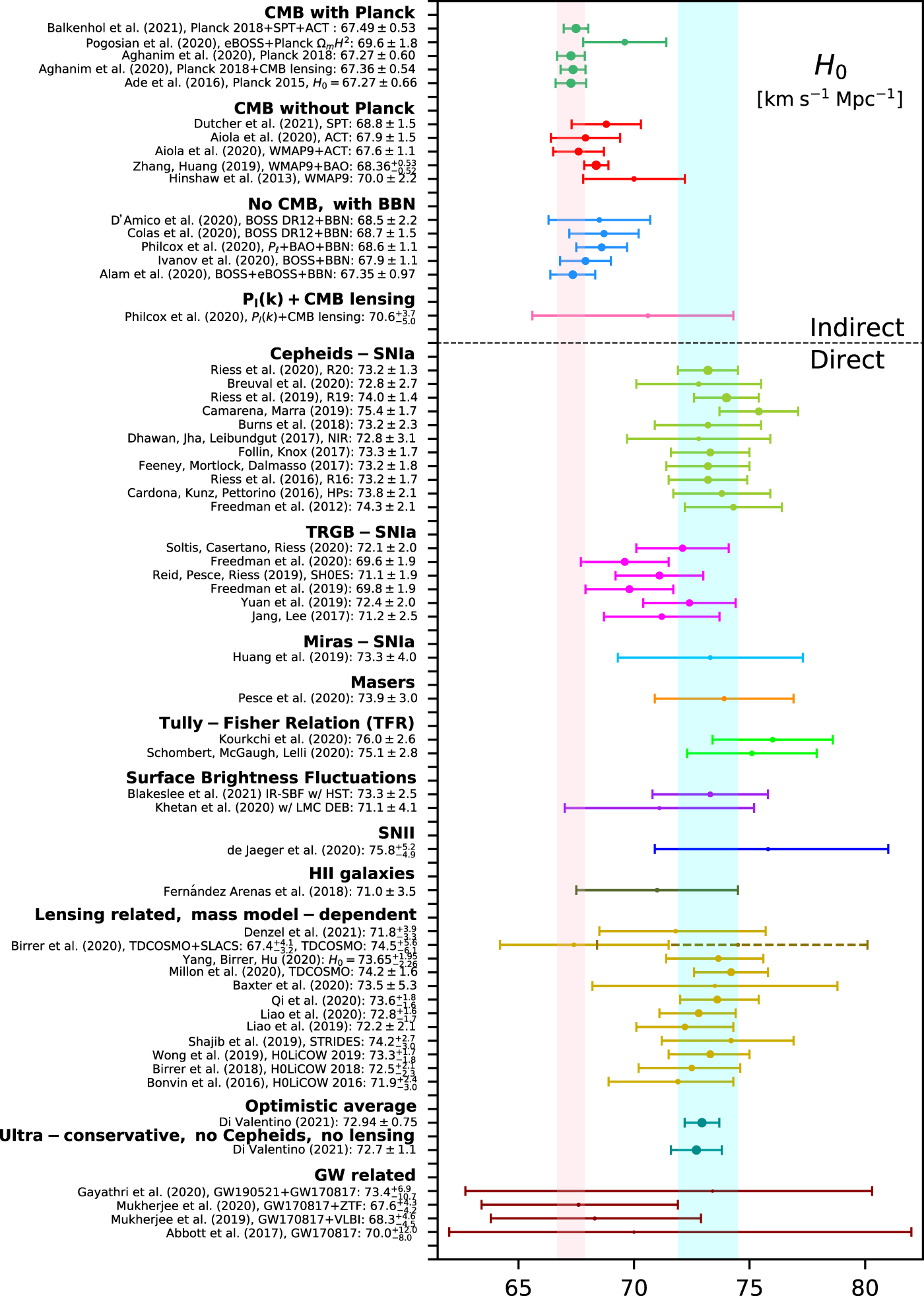
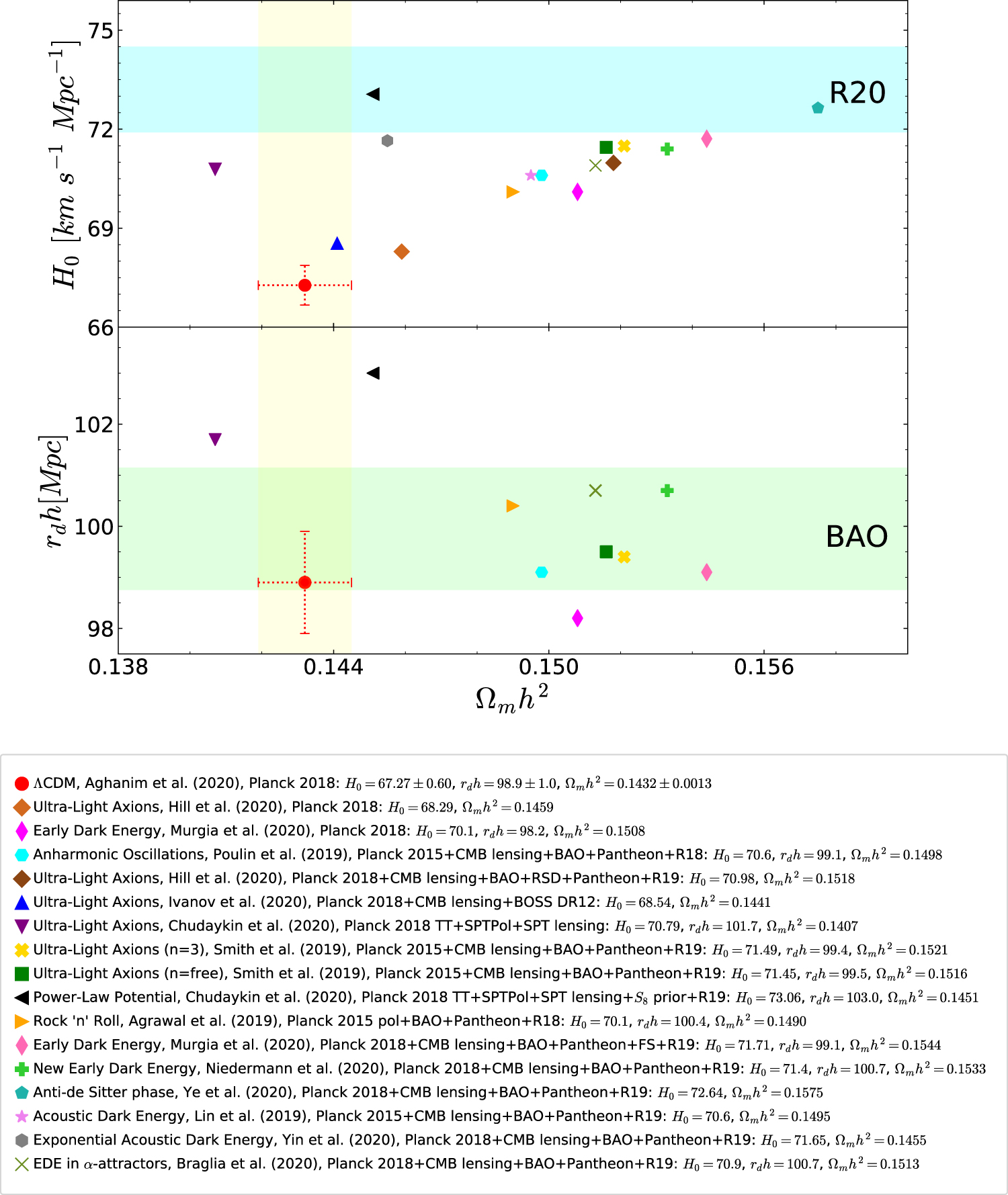
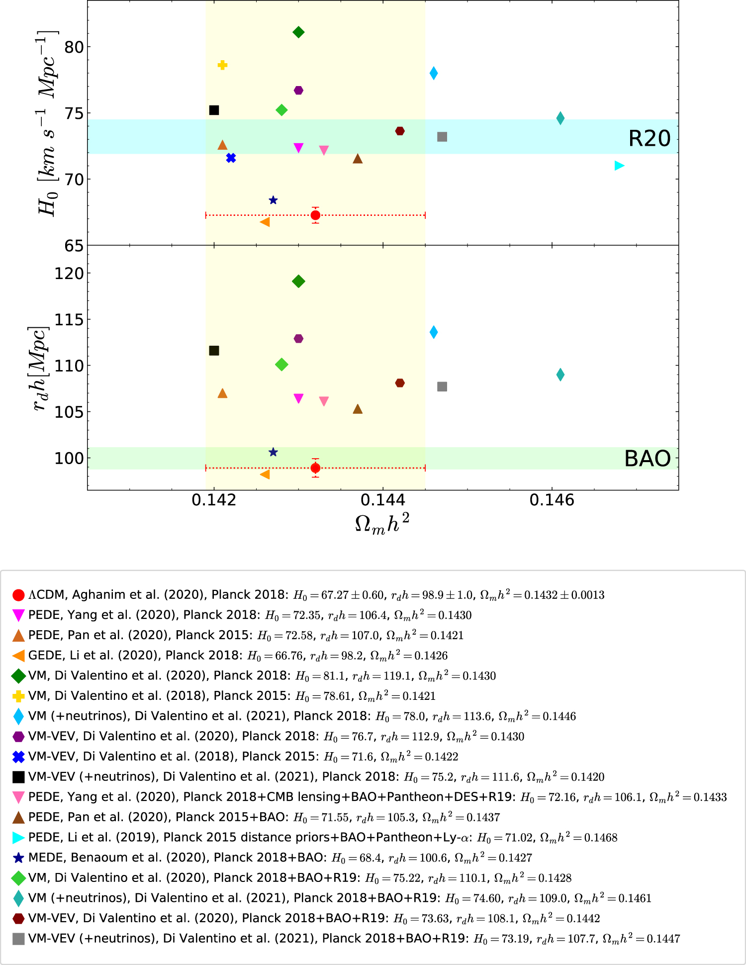
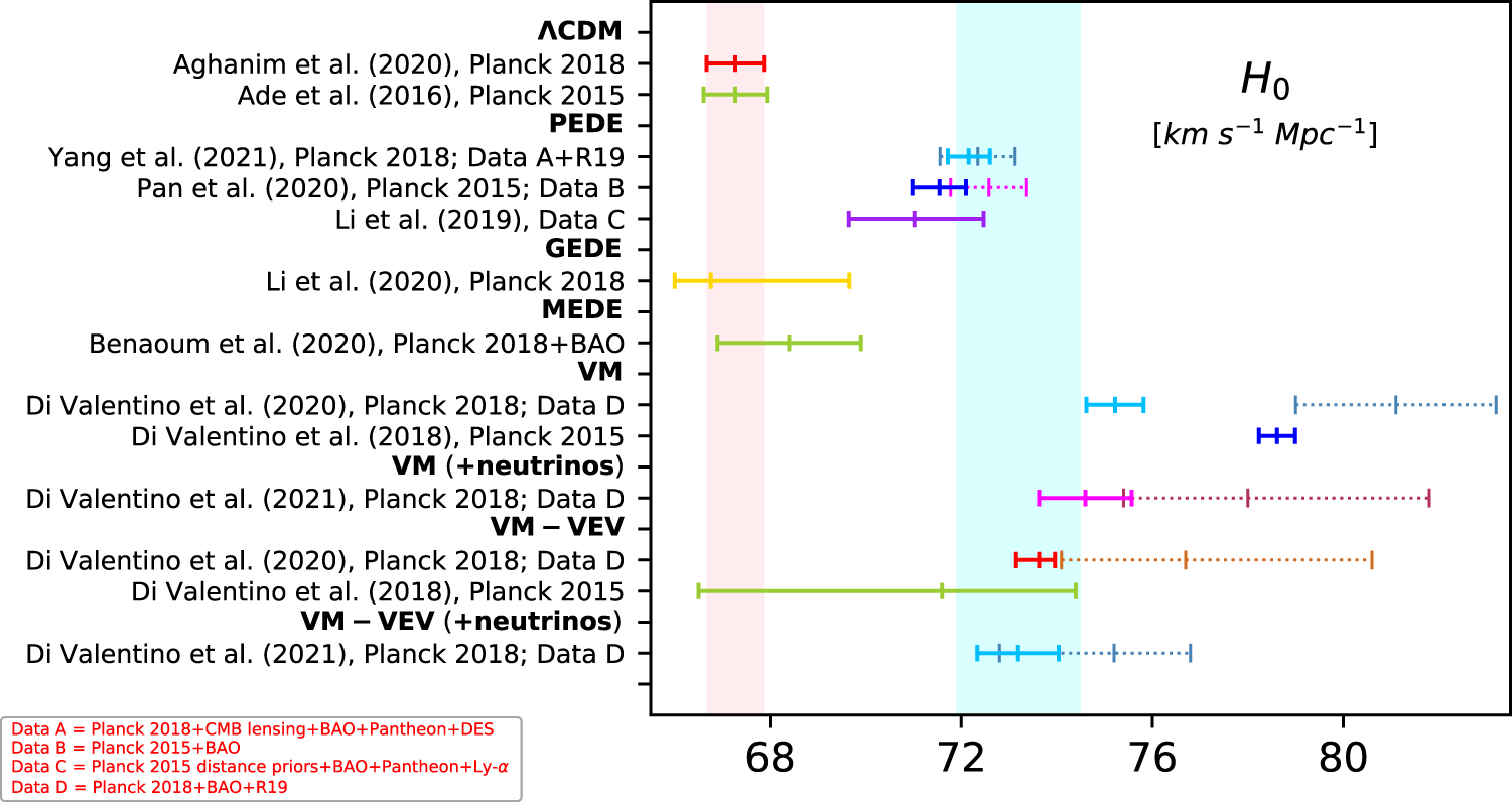
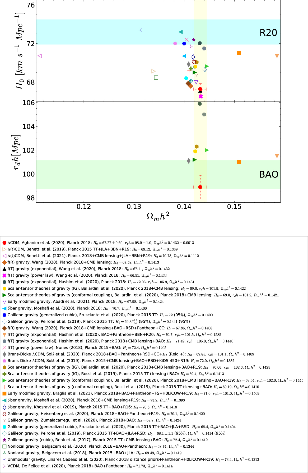
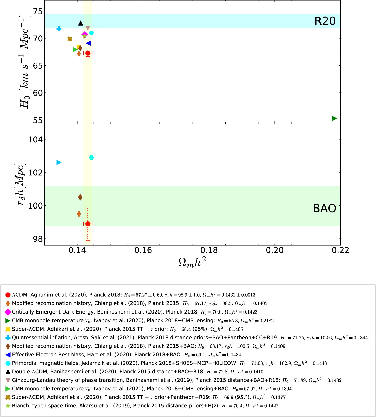
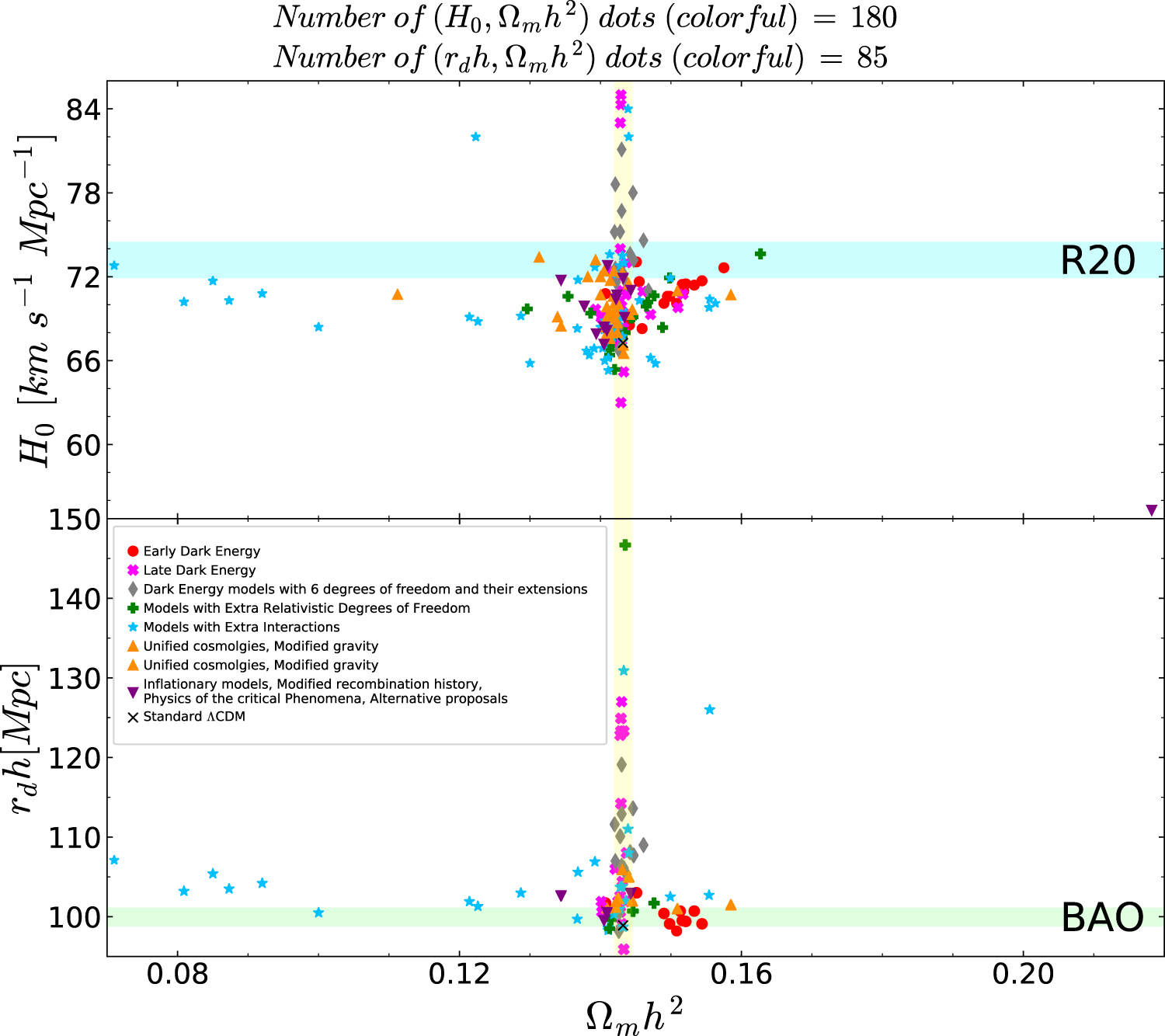