
Abstract
In order to clarify controversial reports on the Fe–Re phase diagram, a new experimental investigation has been carried out. Three intermetallic phases have been evidenced, including the new report of the P phase found for the first time in a binary system. The phase relations involving the σ phase were established. In parallel, a first-principles study has been performed which provided the heat of formation of every ordered configuration for four intermetallic phases (D8b, A12, A13 and P). The mixing energy of solid solutions (fcc, bcc, hcp) was calculated using the special quasi-random structure method. Calculations were performed with the help of the density functional theory, with and without spin polarization. From these results, in the frame of the Compound Energy Formalism using the Bragg–Williams approximation, the Fe–Re phase diagram has been computed without the use of adjustable parameters. Different thermodynamic parameters obtained experimentally and theoretically, as the site occupancies, are compared. The computed phase diagram presents several differences with the experimental one. To understand these differences, the influence of several parameters on the phase stability, such as the magnetic contribution has been evaluated.
Export citation and abstract BibTeX RIS
For more information on this article, see LabTalk. Changes were made to this article on 29 July 2016. The supplementary material was added.
1. Introduction
Rhenium is a third-row transition metal element in group VII of the periodic table, characterized by the third highest melting point among all elements, which makes it extremely useful in developing high-temperature applications particularly when used as a solid solution strengthening element in superalloys [1]. Its presence in the host matrix improves the creep strength thanks to its excellent high-temperature properties. However, it contributes considerably to the formation of the fragile topologically close packed phases (TCP) [2]. In order to avoid TCP precipitation in industrial alloys, research has been done to derive consistent thermodynamic descriptions [3]. The present work is part of a project aiming to systematically study transition metal binary alloys with Re as the base element [4, 5].
Density functional theory (DFT)-based [6, 7] methods permit the prediction of bulk and defect properties for elemental and multicomponent solids starting merely from the knowledge of the atomic numbers of the constituent atomic species. These methods have demonstrated remarkable accuracy in the calculation of various structural, mechanical and energetic properties of materials, including formation enthalpies, cell parameters and elastic constants [8–10]. Computational thermodynamic methods based on the CALPHAD framework [11] are widely used to model phase stability and phase transformation kinetics in complex multi-component alloy systems [12, 13]. The accuracy and precision obtained from these methods depend sharply on the thermodynamic descriptions that form the basis for calculations of phase stability, i.e. the ability of the models themselves to describe the reality, but also the experimental or theoretical knowledge of the system used to determine the model parameters.
Modelling unexplored systems represents a big challenge as they demand extensive experimental measurements. Recently, it has been demonstrated that such measurements can be aided through the application of first-principles (FP) methods for the direct calculation of alloy thermodynamic properties [14–17]. This becomes possible because ab initio methods demand very limited input data from experiments, such that they reduce significantly the need for costly experimental measurements required in thermodynamic database development. Another, even more important advantage of first-principles methods is their capability to predict thermodynamic properties when direct experimental measurements are difficult, or impossible, due to constraints imposed by sluggish kinetics or metastability. On the other hand, performing first-principles calculations of a binary alloy is challenging, since there are too many structures to simulate. Hence, the phases to be simulated are, in principle, limited to a few in number. These phases have either been observed in recent measurements or represent potential candidates to appear in the phase diagram.
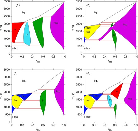
In this framework, the present work focuses on the Fe–Re system which deserves to be more widely understood. The experimental information on this system is partial and uncertain. As shown in figure 1, the published Fe–Re phase diagrams [18–21] are incomplete and controversial. All studies agree on the presence of a σ phase but the reported compositions and homogeneity domains are different. The phase diagram of Iyutina [19] shows two additional intermetallic phases at low temperatures: the χ (A12) and β-Mn (A13) phases. Moreover at the Re-rich end, the Fe solubility limit in hcp is different from that reported by Karup-Mø ller and Makovicky [21].
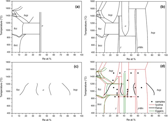
Figure 1. Experimental Fe–Re phase diagrams of (a) Eggers [18], (b) Iyutina [19], (c) Karup-Mø ller and Makovicky [21] and (d) superimposition of the three diagrams together with the black points representative of the samples synthesized in the present work.
Download figure:
Standard image High-resolution imageThe aims of this paper are fourfold:
- (i)to clarify the Fe–Re phase diagram with a new experimental investigation;
- (ii)to estimate the heat of formation by DFT calculations of all the ordered configurations of four intermetallic phases: σ, χ, β-Mn, P;
- (iii)to estimate the enthalpy of mixing of the random solutions (bcc, hcp and fcc), in a 16-atom supercell, using Special quasirandom structures (SQS) methodology [22];
- (iv)to compute the Fe–Re phase diagram, the results of the DFT calculations and the compound energy formalism (CEF) [23], with the fewest adjustable parameters.
In parallel, the σ phase will be investigated in more detail as regards its magnetic and atomic ordering, for which we provide a comparison between the experimental and theoretical site occupancies obtained in the present work.
2. Experimental and computational methods
2.1. Experimental details
All the samples, with nominal compositions indicated in figure 1(d), were prepared from carefully weighed commercial iron (Cerac, 99.9%, 45 µm) and rhenium (Alfa Aesar, 99.9%, 44 µm) powders. The powders were mixed using an agate mortar and a uniaxial pressure was applied to the powders in order to obtain a cylindrical compact (m ≃ 1 g), which was then melted in an arc furnace under an argon atmosphere. Each sample was melted three or four times and rotated upside down between each melting to ensure good chemical homogeneity. After melting, the samples were sealed in a quartz tube under argon and placed in a tubular electrical furnace, at temperatures of 850, 900, 1000, 1050 and 1100 °C, for periods of 8, 7, 6, 5 and 4 weeks respectively and then cooled in water. For annealing at higher temperatures, i.e. ⩾1300 °C, a high frequency induction furnace with a water cooled copper crucible was used. The heat treatment was then performed for eight hours, the temperature was measured with a pyrometer and the samples were quenched by turning off the induction heating. Thus, the samples were cooled in a few seconds. After quenching, the samples were cut, polished and their microstructure and chemical composition were characterized by electron probe microanalysis (EPMA-CAMECA SX100) using pure elements as standards. Large numbers of data points were measured to determine phase composition and homogeneity. To determine the crystalline structure, powder x-ray diffraction (XRD) diagrams were obtained using a Bruker D8-Advance, working in the symmetric Bragg–Brentano geometry, with a rear graphite monochromator used in order to eliminate the fluorescence. The radiation used was Cu-Kα, λ = 1.540 56 Å. The x-ray data collection conditions included 5 ⩽ θ ⩽ 120°, step size of 0.04° and a total counting time of 15 h to obtain high data statistics. The diffractograms obtained were then systematically analyzed by the Rietveld method using the FullProf refinement program.
2.2. Computational methodology
2.2.1. First-principles calculations.
The calculations reported in this work are based on the DFT. They have been performed both for ordered intermetallics and solid solution phases. The total energies were calculated using the Projector Augmented Wave method [24], implemented in the Vienna Ab initio Simulation Package (VASP) [25, 26]. The exchange-correlation energy of electrons was described in the generalized gradient approximation (GGA) using the functional parametrization of Perdew–Burke–Ernzerhof [27]. After necessary tests to control the stability of the energy differences between phases, the energy cut-off for the PAWs was set to 400 meV. These convergence tests for the plane-wave cut-off and the number of the k-points were essential to assure reliable total energy differences [28]. We have intentionally kept the space group fixed whilst relaxing each particular system. As a consequence, a spontaneous lowering of the symmetry was not possible. The total energies of every compound were also minimized in order to equilibrate their volume, assuming a zero pressure environment. Calculations with and without spin polarization (SP) have been considered in the collinear magnetic description.
For the intermetallics, the four phases D8b, A12, A13 and P were considered. These phases were selected as they have been observed experimentally in this system. In particular, the calculation done on the P phase was continued from the experimental study of the present work. This phase would never have been calculated if it had not been evidenced experimentally, particularly because it has never been reported as a binary phase. This is an example of the limitations of systematic high-throughput theoretical approaches such as that adopted by Curtarolo [29] which are always performed within a given set of crystal structures that may never be exhaustive. The crystallographic structures studied are summarized in table 1. The distribution of the two elements (Re,Fe) on the s different sites generates Nφ = 2s ordered configurations which have to be considered for each phase φ. For the complex P phase, because of the huge number of configurations, a simplification has been adopted. All sites of similar coordination number (CN): CN12, CN14 and CN15 + 16 have been merged resulting in only three sublattices of multiplicity 24, 20 and 12 respectively (see table 2) and thus 23 = 8 compounds to compute according to the model (A,F,H,I,J)24(B,C,D,G)20(E,K,L)12.
Table 1. Details of the structures considered in the present study: Strukturbericht, Prototype, Space group, usual name and Nφ, the number of configurations considered in the DFT calculations.
| Strukturbericht | Prototype | Usual name | Space group | Nφ |
|---|---|---|---|---|
| A1 | Cu | γ-Fe, fcc |
 |
7 |
| A2 | W | α-Fe, δ-Fe, bcc |
 |
7 |
| A3 | Mg |  -Re, hcp -Re, hcp |
P63/mmc | 7 |
| D8b | CrFe | σ | P42/mnm | 25 = 32 |
| A12 | α-Mn | χ |
 |
24 = 16 |
| A13 | β-Mn | P4132 | 22 = 4 | |
| — | Cr18Mo42Ni40 | P | Pnma | 23 = 8 |
Table 2. Details of the initial internal position of P-phase structure, oP56, Pbnm, a ≃ 17 Å, b ≃ 5 Å, c ≃ 9 Å, 56 atoms in 12 sites merged into 3 subgroups.
| x | y | z | Site | Wyc | CN |
|---|---|---|---|---|---|
| 0.037 | 0.001 | 0.250 | A | 8d | 12 |
| 0.245 | 0.250 | 0.636 | F | 4c | 12 |
| 0.342 | 0.250 | 0.826 | H | 4c | 12 |
| 0.387 | 0.250 | 0.574 | I | 4c | 12 |
| 0.422 | 0.250 | 0.315 | J | 4c | 12 |
| 0.288 | 0.501 | 0.387 | B | 8d | 14 |
| 0.095 | 0.250 | 0.699 | C | 4c | 14 |
| 0.135 | 0.250 | 0.438 | D | 4c | 14 |
| 0.318 | 0.250 | 0.106 | G | 4c | 14 |
| 0.175 | 0.250 | 0.165 | E | 4c | 15 |
| 0.464 | 0.250 | 0.020 | K | 4c | 15 |
| 0.546 | 0.250 | 0.525 | L | 4c | 16 |
A mesh of 80, 68, 220 and 120 special k-points for σ, χ, β-Mn and P, respectively, were taken in the irreducible wedge of the Brillouin zone for the total energy calculation [30, 31]. Hence, the cell-shape relaxation was considered wherever possible whereas the internal coordinates were optimized using the conjugate gradient algorithm, a highly recommended scheme to relax the ions to their instantaneous groundstate, especially where ionic relaxation is problematic. The stable element reference (SER) states of Fe and Re are their respective ground states: Fe ferromagnetic bcc (α-Fe) and Re nonmagnetic hcp. The enthalpy of formation
 for each configuration in φ phase has been calculated from the total energies, as:

where
 is the total energy of the DFT calculation at 0 K and x, the Re mole fraction.
In this work, the SQS approach was adopted to simulate the fcc, bcc and hcp solution phases. It consists of making a choice on how to match random atomic configurations with a periodic structure. Normally, the optimizing technique, in which the volume, shape and atomic positions are driven by energy and forces/stress minimization, is restricted to the condition where the structure keeps its original symmetry. Hence, we have relaxed the relevant phases, keeping the original symmetries allowing only volume and ionic relaxation for the cubic cell. An additional step has been performed allowing cell shape relaxation for the hexagonal structure. The SQS structures of fcc, bcc and hcp were taken from [32–34], without any further adaptation. A mesh of 172, 144 and 250 special k-points for fcc, bcc and hcp, respectively, were taken in the irreducible wedge of the Brillouin zone for the total energy calculation. In addition to compounds calculated by the SQS methodology for 25, 50 and 75% compositions, we have also simulated dilute solutions using a 16 atom supercell containing 15 similar and 1 dissimilar atom, corresponding to 6.25% and 93.75% of Re. Discrepancies between the first-principles and the CALPHAD values [35] for the lattice stabilities have often been noticed and have been discussed elsewhere [36, 37]. In order to address this issue, mixing parameters are used rather than the SQS-formation energies. The mixing enthalpy
 of each composition has been calculated from the relative total energies as:

where
 and
and
 are the energies of the pure elements in the φ phase under consideration.
To automatically generate first-principles input files of all the ordered configurations of the given crystal structures generated, by assigning each element to each crystal site, the script-tool 'ZenGen' was used [38].
2.2.2. Continuous thermodynamic modelling.
In order to use the DFT results to calculate a phase diagram, continuous thermodynamic models have to be introduced. The Gibbs energy of the solution phases (fcc, bcc, hcp and liquid) has been expressed through a regular solution model as follows

In order to describe the evolution of the relative stability of the different phases, the lattice stabilities of the scientific group thermodata Europe (SGTE) [35] have been used for
 . The mixing energy of the solution has been expressed by a Redlich–Kister expression
 , where the SQS results have been used to estimate
 parameters. The magnetic contribution, Gmag, was taken from the pure SGTE description without binary excess contribution. The separation of the magnetic contribution implies that the expression of the lattice stabilities,
, describes the paramagnetic state of the elements yielding some difficulties when trying to extract FP information to use in this formalism as discussed by Körmann et al [39].
parameters. The magnetic contribution, Gmag, was taken from the pure SGTE description without binary excess contribution. The separation of the magnetic contribution implies that the expression of the lattice stabilities,
, describes the paramagnetic state of the elements yielding some difficulties when trying to extract FP information to use in this formalism as discussed by Körmann et al [39].
The Gibbs energy of the intermetallic phases for a mole of formula unit has been expressed in the modified-CEF [40] i.e. as follows:

with


This approach splits the Gibbs energy of the phase under consideration into two contributions: GCIφ(xi) and
 . GCIφ(xi) is the molar configuration independent contribution; it is a function of the overall composition of the phase expressed by xi the molar fraction of the element i. It is multiplied by the number of moles of the atom in a formula unit of the phase, ∑sas, as being the multiplicity of the site s.
 corresponds to the Gibbs energy of the pure element i in the φ structure. In the present work, they have been expressed using the DFT results as follows:

 comes directly from the DFT results while
 is the SGTE lattice stability for the pure element i in its SER state.
 is the difference of vibrational entropy of i between the two structures φ and SER. The influence of this term will be discussed in the last part of this work. The last term,
 , is introduced to take into account that the temperature dependence
describes the paramagnetism of the SER state while,
, is introduced to take into account that the temperature dependence
describes the paramagnetism of the SER state while,
 is obtained for the ferromagnetic state. This term will only be used for the magnetic elements, i.e. only for Fe in the present case. In the present work, a constant value of −9.5 kJ.mol−1 was used, allowing us to reproduce the FP results with the stable configuration enthalpy curves calculated at low temperature.
The first term of GCIφ(xi) thus corresponds to the mechanical mixture of pure elements in the φ structure. The second term
 corresponds to an excess term from the interaction of the element i and j independent of the configuration. This term has not been used in the present work. Gmag is the magnetic contribution. It is expressed with the same relation as for the solid solutions in equation (3). Its influence will be discussed in the results section for the case of the σ phase.
is the configuration dependent contribution function of the site fractions.
 stands for the fraction of the element i in the site s. The first term of this contribution expresses the sum of the Gibbs energy of formation of all the compounds, C, defined by the model weighted by a site fraction product. When calculating the site fraction product for the compound C, the element i occupying the site s in C has to be considered for each site.
 is the Gibbs energy of formation of the stoichiometric compound C referring to the pure elements in the phase φ. The second term corresponds to the ideal configurationnal mixing.
During this work, the Gibbs energy of formation of the stoichiometric compound C has been expressed using the results of DFT calculation for this configuration making the assumption that the difference of total energies at 0 K corresponds to the difference of the enthalpies.


where the
 takes the element i present on the site s in the compound C under consideration. In the present work,
 were not considered. The vibrational entropy of the stoichiometric compounds is thus the weighted mean of the value for the pure elements in φ structure.
As a first approximation, The Gibbs energy is calculated at a finite temperature using the Bragg–Williams Approximation (BWA). In this approximation, BWA considers that both interactions within sublattices and non-configurational entropies are negligible; i.e. only the mixing entropy is considered.
3. Results and discussion
3.1. Experimental investigation
Table 3 lists experimental results for the most important samples. At 850 °C, the two samples with compositions Fe73Re27 and Fe68Re32 clearly show equilibrium between the bcc phase and a new phase with composition close to Fe60Re40 evidenced by EPMA. This phase cannot be indexed on the basis of the χ phase as proposed by Iyutina [19]. On the contrary, a careful analysis performed with the search/match software EVA shows that it can be indexed by the P phase reported in Cr–Mo–Ni [41, 42]. A Rietveld analysis confirmed this point. The crystal structure of this phase with 12 distinct crystallographic sites is so complex that a complete refinement of the crystal structure, including site occupancies on all sites and 26 variable atomic coordinates cannot be performed with much accuracy. Nonetheless, it is clear from figure 2 that the structure model of Shoemaker et al is able to reproduce most features of the crystal structure of our sample confirming the phase identification. Other samples with higher rhenium content were synthesized and annealed at the same temperature. Their analysis shows the following phase sequence: P, β-Mn and hcp. The composition of β-Mn is confirmed to be close to Fe40Re60 as proposed by Iyutina [19]. A significant homogeneity domain has been observed for neither the P nor the β-Mn phases. In each of these samples, however, traces of the hcp phase has been observed, even when this phase should not appear. It is probably conserved from the high temperature solidification and not completely removed by the annealing treatment. These samples are not presented in table 3. At 900 °C, the P phase is still present and the σ phase does not show up. At 1000 °C, the σ phase is present and traces of the β-Mn phase are visible in the sample Fe55Re45 (see table 3). At 1050 °C, neither the P nor β-Mn phases are observed. At this temperature and above the σ phase is always in equilibrium with the Re-based hcp solid solution on the Re rich side. On the Re poor side, the phases indicated in table 3 are the phases as observed in the XRD pattern measured at room temperature after quenching. It is not certain that they correspond to the equilibrium phases since the solid solutions based on iron may transform during quenching. In particular, at 1300 °C and 1500 °C two phases are observed with the same compositions Fe75Re25 and the two structures bcc and hcp. The presence of a hcp phase at this composition close to the iron border confirms the interpretation made by Okamoto [20], of the results of Eggers [18], that this phase should be derived from metastable hcp iron, though several inconsistencies concerning the metastable extrapolation of the solvus lines to pure iron were noticed. Note that Iyutina [19] (not cited in the review by Okamoto) did not identify the crystal structure of this phase. The presence of a bcc phase of the same composition in the same sample may be an indication that the hcp phase has not been retained completely by quenching. From these results, we may propose the tentative updated phase diagram of figure 3, discussed in the following section.
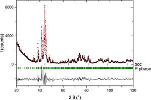
Figure 2. XRD pattern of sample Fe68Re32 annealed at 850 °C compared to the structure model of the P phase from [41, 42] in a Rielveld-like analysis including the bcc phase (difference below). No complete structure refinement of the P phase was attempted.
Download figure:
Standard image High-resolution image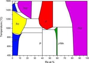
Figure 3. Tentative experimental Fe–Re phase diagram.
Download figure:
Standard image High-resolution imageTable 3. Experimental conditions for the synthesis and metallurgical characterization. Standard deviations on compositions are indicated between brackets. A typical standard deviation on lattice parameters is 0.001 Å.
| Overall Re at.% | Heat treatment | Phase | Re at.% | Lattice parameters Å−1 |
|---|---|---|---|---|
| 27 | 850 °C, 6 weeks | bcc | 9(1) | a = 2.892 |
| P | 39(1) | a = 8.977 b = 16.795 c = 4.685 | ||
| 32 | 850 °C, 6 weeks | bcc | 9(1) | a = 2.893 |
| P | 40(2) | a = 8.977 b = 16.797 c = 4.685 | ||
| 45 | 1000 °C, 6 weeks | σ | 50(1) | a = 9.111 c = 4.749 |
| β-Mn | 55(2) | a = 6.433 (traces) | ||
| 30 | 1050 °C, 5 weeks | bcc | 19(3) | a = 2.911 |
| σ | 37(2) | a = 9.020 c = 4.693 | ||
| 45 | 1050 °C, 5 weeks | σ | 51(2) | a = 9.115 c = 4.752 |
| hcp | 70(3) | (traces) | ||
| 25 | 1100 °C, 4 weeks | bcc | 18(1) | a = 2.917 |
| σ | 35(1) | a = 9.039 c = 4.705 | ||
| 56 | 1100 °C, 4 weeks | hcp | 79(3) | a = 2.716 c = 4.379 |
| σ | 54(1) | a = 9.146 c = 4.772 | ||
| 65 | 1100 °C, 4 weeks | hcp | 80(1) | a = 2.720 c = 4.390 |
| σ | 54(1) | a = 9.147 c = 4.774 | ||
| 24 | 1300 °C, 8 h | bcc | 25(1) | a = 2.939 |
| hcp | 25(1) | a = 2.595 c = 4.201 | ||
| 45 | 1300 °C, 8 h | σ | 46(1) | a = 9.095 c = 4.739 |
| 25 | 1500 °C, 7 h | bcc | 25(1) | a = 2.942 |
| hcp | 25(1) | a = 2.604 c = 4.204 | ||
| 34 | 1500 °C, 7 h30 | bcc | 25(1) | a = 2.932 |
| σ | 39(1) | a = 9.044 c = 4.710 | ||
| 50 | 1500 °C, 8 h | σ | 52(1) | a = 9.133 c = 4.766 |
| hcp | (traces) | |||
| 60 | 1500 °C, 8 h30 | hcp | 72(1) | a = 2.716 c = 4.376 |
| σ | 54(1) | a = 9.175 c = 4.795 |
3.1.1. Experimental phase diagram.
The proposed phase diagram in figure 3 is limited to the temperature range studied in the present work. The experimental study of this system is particularly difficult. This is due to the fact that some phases that cannot be quenched (fcc and hcp) transform completely or partly by a martensitic transformation into the bcc phase. Other phases (σ, P) have quite complex crystal structures making their identification from XRD difficult when present simultaneously. Moreover, their identification by EPMA is also difficult as their compositions are similar; P and β may both have the composition of σ. Also, rhenium is very much a refractory element. The determination of the melting equilibria is difficult. The reactions at low temperature, in particular in the range 900–1100 °C where the invariants involving σ, P and β are located, are sluggish and the equilibrium is difficult to establish. This means that we are still far from having completely established the phase relations in the whole composition and temperature ranges. However, we believe we have clearly established new facts that are important for understanding this system. These are summarized below:
- the existence of the P phase which has never been reported in Fe–Re and, as far as we know, it is the first time that this structure type is evident in a binary system;
- non existence of the χ phase as previously reported;
- the martensitic nature of the transformation from hcp to bcc;
- the homogeneity range of the σ phase at high temperature (1100–1500 °C) larger than previously reported and the nature of the equilibria with other phases, including the absence of χ and β-Mn in this temperature range as reported before;
- reliable site occupancies have been obtained in the complete homogeneity range of the σ phase which makes Fe–Re one of the systems in which the σ phase has been best characterized (see below).
3.1.2. Experimental σ site occupancies.
The large x-ray scattering contrast between Re and Fe allows us to precisely determine the Re occupancy on the five different sites in the σ phase of samples annealed from 1000 to 1500 °C (figure 4) by using the Rietveld refinement. The results are presented in a table in the supplementary material. All the sites show a mixed occupation in the studied composition range; this is characteristic of a rather low degree of order. The different site occupancies are clearly separated except for those of 2a and 8i2. Sites 4f and 8i1 are preferentially occupied by Re and site 4f of the highest coordination number (CN15) has the highest Re content. Site 8j is close to being randomly occupied. Sites 2a and 8i2 are preferentially occupied by Fe. This is basically attributed to an atomic size effect: the largest atom shows a preference for sites with a large coordination number [43].
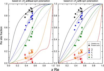
Figure 4. Comparison of σ phase experimental (symbols) and calculated (lines) site occupancies computed at 1500 K. The calculated ones are computed with Bragg–Williams approximation (BWA), based on the DFT heats of formation with and without spin polarization. The dashed line indicates a fully random occupation.
Download figure:
Standard image High-resolution imageOur results are in excellent agreement with the recent paper of Cieslak et al [44], as shown in figure 4, with a very comparable scattering of occupancies in the two datasets; however, we strongly extended the studied composition range.
3.2. Theoretical study
The details about relaxed crystallographic structures (cell parameters, internal atomic positions) and total energy with corresponding enthalpy of formation and magnetic moment for all the studied phases are given in the supporting materials.
3.2.1. Solid solutions interactions.
The SQS derived enthalpies of the fcc, bcc and hcp phases, calculated without (blue symbols) and with spin polarization (red symbols) are displayed in figure 5. For the fcc and bcc phases, the states considering the spin polarization are more stable than those without SP while there is no difference for the hcp phase. The fcc and bcc phases are thus stabilized by magnetic ordering while the hcp phase is not. Otherwise, the fcc and hcp phases present similar behaviours. The mixing energies in these phases are essentially positive indicating repulsive interactions; they become slightly negative only for composition close to pure Fe.
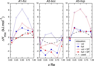
Figure 5. Enthalpy of mixing in the Fe–Re solid solutions calculated using SQS calculations (fcc, bcc and hcp), employing several schemes: volume (empty symbol) and full (filled symbol) relaxation, with and without spin polarization (SP). The dashed lines represent the fitted excess energy considered in the computed phase diagram. The different solid lines are drawn to guide the eye of the reader.
Download figure:
Standard image High-resolution imageEquation (3) was considered to model the mixing enthalpy in the solution phases: fcc, bcc and hcp, based on the SQS results obtained with spin polarization, after full relaxation. However, because of the dynamical instability of Re in bcc [45, 46], only volume relaxation results have been considered for the bcc phase. A single regular 0L interaction term has been chosen for the bcc and hcp phases equal to 0Lbcc = −7 and 0Lhcp = +7 kJ.mol−1. Because of the stronger asymmetrical shape for the fcc structure, an additional term has been considered yielding 0Lfcc = +3 and 1Lfcc = −10 kJ.mol−1. The dashed lines in figure 5 represent the resulting enthalpy curves for the different solution phases. The choice made may be considered rather subjective as none of the SQS sets follow a very regular behaviour. However, it is expected that they indicate an order of magnitude allowing us to build a reasonable thermodynamic database.
3.2.2. Intermetallic phase stability.
The formation enthalpies of all the configurations calculated for the four phases, σ, χ, β-Mn and P phases are shown in figure 6. For each phase, a solid line is drawn between the configuration of lowest energy; it corresponds to the so-called convex hull. Two sets of results corresponding to different approximations are shown: with and without spin polarization. The spin polarized calculations are expected to describe the 0 K and low temperature energetics more precisely. The results obtained without spin polarization help us to understand more clearly what happens at higher temperatures where the magnetic ordering vanishes. All the phases have significantly lower enthalpies in the spin polarized calculation. This stabilization is weaker for configurations with higher Re content.
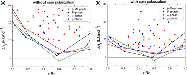
Figure 6. Formation enthalpies of all ordered configurations of the σ, χ, β-Mn and P phases, i.e. 32, 16, 4 and 8 compounds, respectively, without (left panel) and with spin polarization calculations (right panel). The solid lines show the groundstate of each phase.
Download figure:
Standard image High-resolution imageBoth approximations predict the stability of only one intermetallic phase at 0 K: the β-Mn phase with a negative enthalpy of formation of −1.8 kJ.mol−1 in the spin polarized and −1.72 kJ.mol−1 in the nonmagnetic calculations. The stability of this phase, at low temperature, is in agreement with the experimental observations at low temperatures by Iyutina [19] and in the present work. Moreover, the minimum of the β-Mn phase convex hull corresponds to the configuration with Fe in CN12 and Re in CN14, at xRe = 0.6, very close to the composition reported experimentally for this phase. The stability of the P phase at low temperature can be understood from the fact that its convex hull is the lowest in energy after the β-Mn phase. However, according to the present DFT results, this stability should not extend down to 0 K. Moreover, the closeness of the different convex hulls explains that the structures not stable at 0 K may appear at a high temperature.
In the following, we analyze the energetic dependence of the σ phase configurations as a function of the (Fe,Re) occupations of its five sublattices. The configuration FeReReFeRe4, lying on the convex hull has the lowest formation enthalpy, as predicted by spin polarized calculations. It is however very close to the ReReReFeRe configuration that is the most stable in the approximation without SP. The most stable σ phase groundstate configurations correspond to those with the high CN sites occupied by Re, while icosahedral sites are occupied by Fe. Among these, the most stable configuration corresponds to the composition Re2Fe (i.e. FeReReFeRe). Even for this configuration the calculated enthalpy value is positive indicating that the σ phase is not stable at 0 K relative to Fe and Re in their respective ground states, in agreement with the experimental observation.
Within the BWA at 1500 K, the σ site occupancies have been computed using the two sets of heat of formation, with and without spin polarization. Figure 4 shows a good agreement between the experimental and calculated data, confirming the reliability of both the calculation and experimental measurements. The agreement is slightly better with the non-spin polarized calculations. This is understood by the fact that at the experimental temperature, the σ phase is not magnetic. This satisfactory explanation raises the question of the best DFT dataset to use within the continuous thermodynamic models. The results using spin polarization (SP) approximation would describe the low temperature region better and fails to reproduce the experimental results at finite and high temperatures. Linking both regimes in a continuous way constitutes one of the challenges of the use of DFT results in the CALPHAD approach.
During the calculations, the relaxed cell parameters of the different phases are also obtained and can be found in the tables in the supplementary material. The composition dependence of the cell parameters manifests a quasi-linear behaviour. They increase upon replacing Fe with Re. For the σ phase, the c/a ratio fluctuates around 0.52 with a deviation at xRe = 0.4. In fact, site 8j of CN14 is characterized by a very short inter-atomic distance along the z-axis, which renders it different from its analogue, 8i1 of CN14. This explains the different occupancy observed experimentally between these two sites. Another interesting feature is the negative deviation of the atomic volume from the Vegard's law. This behaviour is attributed to binding and short bond lengths which occur when Re atoms preferentially occupy high CN sites in the σ phase structure.
3.2.3. Magnetic entropy of the σ phase.
Within the GGA and for non-spin polarized (nonmagnetic) calculations, Korzhavyi et al [47] and Havránková et al [48] predicted the lattice stability of σ Fe to be 38.2 and 40.6 kJ.mol−1, respectively, which is at variance with our prediction, 25.65 kJ.mol−1. We attribute this striking disagreement to the internal coordinates and the tetragonal ratio which were held fixed at the experimental values (taken from σ-CrFe stable composition [49]), throughout the calculations of [47, 48]. In the same study Korzhavyi et al [47] demonstrated the importance of a spin polarized treatment of the paramagnetic state of iron-based σ phases. They modelled the paramagnetic state employing the Disordered Local Moment (DLM) [50] approach based on the Coherent Potential Approximation (CPA) [51]. The electronic structure calculations were based on DFT and the Korringa–Kohn–Rostoker (KKR) method [52, 53], in conjunction with the Multipole-corrected Atomic Sphere Approximation (ASA + M) [54]. After applying this procedure, the σ Fe lattice stability reduced to 21 kJ.mol−1. This points out the importance of calculating the enthalpies of iron-based σ phases in a spin polarized paramagnetic scheme.
The average magnetic moment of every configuration obtained by DFT is shown in figure 7(a). The dotted red line links the most stable ones and the full red line links the configuration on the convex hull.
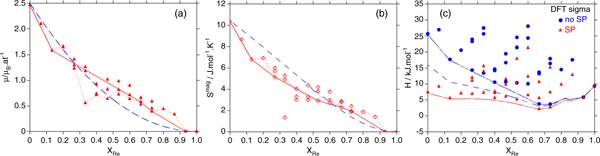
Figure 7. (a) Average magnetic moments, (b) magnetic entropies and (c) formation enthalpies obtained using DFT and CALPHAD approach, see the text for more details.
Download figure:
Standard image High-resolution imageTo estimate the magnetic entropy contribution to the Gibbs energy at high temperatures where σ Fe–Re is experimentally observed, we assumed the crude hypothesis that Fe and Re (induced)-magnetic moments, calculated at 0 K in a spin polarized ferrimagnetic solution,
 , conserve their values at high temperatures where σ is stable in the paramagnetic state. The magnetic entropy is approximated, at high temperatures [39], as:

The DFT magnetic entropy for each configuration, calculated using equation (10), is shown in figure 7(b) as red rhombuses. The red dotted line connects the magnetic entropies that belong to the most stable configurations and the solid red line connects those belonging to the convex hull, while the blue dashed line corresponds to the magnetic entropy determined by the CALPHAD approach. It has the most pronounced values in the Fe-rich side and decreases in a quasilinear behaviour upon replacing Fe by Re atoms in the different sublattices.
In the rest of this section, we show how we modelled the enthalpy in the finite temperature limit, based on CALPHAD methodology and starting from the DFT-inputs, namely the magnetic moments. This modelling is necessary to simulate the finite-temperature section of the phase diagram. The blue dashed line represented in figure 7(a) corresponds to the magnetic moment calculated using the magnetic contribution introduced in equation (5). It is expressed by the classical magnetic contribution to the Gibbs energy used in the CALPHAD approach introduced by Hillert and Jarl's expression [55] based on Inden work [56]. In this contribution, the averaged magnetic moment is a function of the composition of the phase.

The dashed blue curve in figure 7(a) is obtained using
 ,
,
 and
and
 . The magnetic energy contribution is determined by the fit to the magnetic moment. Using this contribution together with the 0 K non-spin polarized DFT enthalpies allows us to model the formation enthalpy in the finite temperature limit. This is illustrated in the blue dashed curve of figure 7(c), where the enthalpies are less positive than the DFT non-spin polarized ones. The red curve is calculated using the DFT results in the spin polarization approximation. The full blue curve corresponds to the case using the DFT results without spin polarization, without CALPHAD magnetic contribution. The dashed blue curve is calculated adding to this one the magnetic contribution. The shift from the full blue line is determined by the fit to the magnetic moment. It comes quite close to the red curve calculated with SP, in particular in the range where the phase is the most stable. A good agreement between the magnetic entropies determined by the DFT (solid red line) from equation (10) and the one determined by CALPHAD (blue dashed line), is shown in figure 7(b).
3.3. Computed phase diagrams
To compute the Fe–Re phase diagram, we have chosen to use the empirical input constituted by the SGTE pure element description. Even if many of the thermodynamic behaviours of the phases have been determined in our FP calculations, thermally-induced vibrational effects allowing us to expand the system have not been calculated. It is thus impossible to calculate the transition of the pure Fe or the melting. The bcc and hcp phases are set as reference states for Fe and Re respectively. Files to reproduce the phase diagrams are available in the supplementary material.
The first tentative diagram has been computed from the fcc, bcc, hcp and liquid solutions of pure elements without any interaction parameters. The σ, χ, β-Mn and P intermetallic phases have been described in the CEF with all the end-member compounds calculated by DFT with spin polarization. The mixing in each sublattice is considered as ideal, only the configurational entropy (BWA) is taken into account. The result is shown in figure 8(a). The phase diagram presents some similarities with the experimental information. The Fe solubility in the Re hcp phase is limited. The β-Mn and P phases are stable at rather low temperature and at compositions close to the measured ones. Their composition ranges are however wider than they are experimentally. A striking disagreement appears with the stabilization of the σ phase for the pure Fe. As already noticed in the section discussing the comparison of the experimental site occupancies for this phase, the SP scheme does not describe very well the σ phase in its stable temperature range. The way the SP energies are taken into account in the CEF does not allow us to account for the magnetic transition and overestimates the stability of the σ phase at high temperature for Fe rich compositions.
Figure 8. Tentative computed phase diagrams: (a) without excess parameters for the solution phases using the DFT results with SP for the intermetallic phases, (b) without excess parameters for the solution phases using the DFT results without SP for the intermetallic phases, (c) with excess parameters from SQS for the solution phases using DFT without SP for the intermetallic phases and (d) as in (c) with additional vibrational entropies for the pure elements in the intermetallic phases.
Download figure:
Standard image High-resolution image
The same assumptions using the DFT results without the SP scheme allow us to calculate the phase diagram as shown in figure 8(b). The σ phase then totally disappears, as well as the P phase. The only remaining intermetallic phase is the β phase stabilized for compositions close to the experimental one. The Fe solubility in the hcp phase is overestimated at high temperature, but the appearance of this phase at high Fe content points to its metastability in this region.
Another calculation of the phase diagram has been made using excess parameters for the solid solutions based on the SQS results as shown in the earlier section (figure 5). The interaction in liquid has been considered equal to that in the bcc phase. The calculated phase diagram is presented by figure 8(c). In contrast to the modelling without any additional parameters, it presents a better agreement with the proposed solubility of Fe in hcp and of Re in bcc and fcc. The temperature range is not in very good agreement but considering the approximation we applied to derive the excess parameters from the SQS information, it is indeed a fair result.
The last phase diagram was calculated by adding the differences of vibrational entropy,
, introduced in equation (7). This contribution could be estimated by phonon calculations. Attempts to calculate such a contribution for the σ phase have recently been reported by Palumbo et al [57]. However technical problems remain due to the dynamical instability of this phase for pure elements. In order to stabilize the σ phase, the following values have been used:

The values used for the entropy of pure Re corresponds to the one obtained by Mathieu et al in their study of the Mo–Re system [3]. For the P phase,

were introduced.
We have chosen to reduce the β-Mn range using

By using the modified-CEF [40], this addition affects the whole composition range. Thus, these small changes strongly affect the equilibrium of all phases, as is shown by figure 8(d). All the phases reported in the experimental phase diagram now appear. Their range of stability is not precisely reproduced but is in qualitative agreement.
This result is highly encouraging but can also indicate a few directions for improvement. We have already mentioned that the input could constitute the derivation of the vibrational entropy from the phonon calculations. Coming back to the DFT on the ground state of the different phases, we should remember that the structure of the P phase has been much simplified in order to get a reasonable number of configurations to compute. It was shown in the case of the σ phase [3] that the reduction of the number of sublattices induces the need of excess parameters in the merged sites. This could be an alternative to the rather high extra vibrational entropy introduced for the pure iron P phase. The possible need for excess parameters could also be studied for the β phase. Due to the rather simple structure of this phase, close neighbours are located on sites belonging to the same sublattice. Excess interactions that have been shown to be repulsive by SQS for some phases in the Re rich area could thus also destabilize this phase a bit and shrink its homogeneity range.
In spite of our efforts, we could not make the hcp phase appear on the iron rich side of the phase diagram. This is mainly due to the repulsive nature of the two elements in this structure. However, as can be seen in figure 8(c), the bcc phase instead appears at high temperature, domain in the range xRe ≃ 0.3, 1450 < T < 1700 K. As we mentioned in the relevant experimental results section, the hcp phase was always mixed with the bcc after quenching from a high temperature. This was interpreted as a martensitic transformation (hcp to bcc) during quenching, mainly based on the hypothesis made by Okamoto [20] that this phase, reported by Eggers [18] and Iutina [19], is hcp. However, an alternative explanation is also plausible: the bcc phase could be the stable phase at high temperature and would transform into hcp during quenching. In this case, the ab initio study would question the experimental phase diagram. Additional measurements of this region of the phase diagram are probably needed but would be difficult because they should be conducted in situ at very high temperatures.
4. Conclusions
In the present work, the phase diagram of Fe–Re system was studied both experimentally and theoretically. This is a challenging system since it includes complex phase structures and magnetism.
The experimental updated diagram does not include the χ phase but an orthorhombic P phase found for the first time in a binary system. The γ-Fe (fcc), σ, (hcp), β-Mn homogeneity domains are different from those proposed in previous studies.
In the DFT frame, calculations have been made to determine the heat of formation of all ordered configurations of the four intermetallic phases and the mixing enthalpies of the three solid solutions (SQS approach). From these results, we have tried to answer the question: Could we build a reasonable phase diagram from the only theoretical calculation results, without any assessed parameter? Several encouraging attempts have been presented. Because of the close groundstate of intermetallics, any additional small contribution, could drastically change the phase equilibrium. This shows that the Fe–Re system is very sensitive and deeper investigation is required to consider the magnetic contribution and its temperature dependence from the only DFT input.
The Re site occupancies were determined both experimentally and by theoretical calculation in BWA. Remarkable agreement was found between experimental observations and theoretical calculations and confirms that Re shows a preference for high coordination sites.
Finally, this work raises several questions of interest for phase diagram calculation: (i) the choice between the DFT results obtained with or without spin polarization; (ii) the lack of a consistent description of a pure element from 0 K, including magnetism; (iii) how to deal efficiently with the magnetic contribution of ordered phases.
Acknowledgments
Financial support from the Agence Nationale de la Recherche (Project Armide 2010 BLAN 912-01) is acknowledged. The DFT calculations were performed using HPC resources from GENCI-CINES (Grant 2013-96175).
Footnotes
- 4
The order of the elements for the σ corresponds to 2a 4f 8i1 8i2 8j.