
Abstract
The properties of the weakly bound S(L = 0)-state in the  ion are investigated with the use of the results of highly accurate computations. The hyperfine structure splitting of this ion is investigated. We also evaluate the lifetime of the
  ion against the nuclear (d, t)-fusion and discuss a possibility of evaluating the corresponding annihilation rate(s).
Export citation and abstract BibTeX RIS
1. Introduction
The boundness of the Coulomb three-body system with unit charges formed by the triton t (or tritium nucleus), deuteron d (or deuterium nucleus) and one negatively charged antiproton  was discussed in a number of our earlier studies [1, 2]. It was shown that this system is certainly bound. However, it was also found that the
  ion has only one bound (ground) S(L = 0)-state and this state is, in fact, a weakly bound state. According to the definition of weakly bound states, the ratio of the binding energy ε to the total energy E of each of these states is very small, i.e.
  . For weakly bound states in Coulomb few-body systems, the dimensionless parameter τ must be less than 0.01 (or 1%). A number of Coulomb three-body systems (ions) with unit charges have some weakly bound states. For instance, the P*(L = 1)-states (excited P-states) in the ddμ and dtμ ions are extremely weakly bound. However, the ground S(L = 0)-states are weakly bound only in a very few such systems. In particular, the ground S(L = 0)-state in the three-body
  ion is weakly bound. It makes the
  ion unique among all Coulomb three-body systems with unit charges, since it contains three heavy particles, but has a very small binding energy.
In general, each weakly bound state has a number of extraordinary properties. Our main goal in this study is to investigate such properties of the ground state of the  ion. First of all, we want to investigate the properties which are 'typical' for each weakly bound state in the Coulomb three-body systems with unit charges. As follows from the results of numerical computations of the weakly bound states, many of such properties are substantially mass dependent. Even small variations of particle masses produce noticeable changes in the expectation values of a large number of properties. To avoid this problem, one must use extremely accurate variational wavefunctions. Briefly, this means that the total and binding energies of such a state must be determined to the maximal numerical accuracy which can be achieved in modern bound-state calculations. To achieve this goal, we need to solve the corresponding Schrödinger equation for bound states in the Coulomb three-body system
  to a very high numerical accuracy. The highly accurate wavefunction Ψ obtained during this procedure is used later to compute various bound-state properties of the
  ion. Some of these properties are of great interest in numerous applications involving the
  ion.
ion.
It is clear that the structure of the bound state(s) in the  ion cannot be explained accurately by ignoring contributions from strong interactions between antiproton, deuteron and triton [3]. Indeed, the actual interparticle distances in the ground S(L = 0)-state of the
  ion are only ≈50 times larger than the effective radius of the nucleon–nucleon interactions (or NN-interactions, for short). Therefore, one can expect that the strong components of all (three) interparticle potentials in the
  ion can change the computed expectation values, i.e. the bound-state properties. In this study, however, we will ignore all possible contributions from the strong components of all interparticle potentials. Our main goal below is to perform highly accurate analysis of the Coulomb three-body system
  with unit charges. In the next study, we are planning to include more realistic interaction potentials in our analysis.
2. The Hamiltonian and its reduction for weakly bound systems
In the non-relativistic approximation, the Hamiltonian of the three-body  ion takes the form [4]
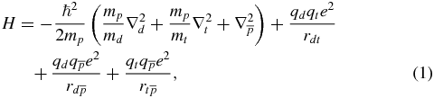
where  and
and  . In equation (1), the notation ℏ stands for the reduced Planck constant, i.e.
  , and e is the elementary electric charge. For the
  ion, it is very convenient to perform all bound-state calculations in proton-atomic units in which
  and e = 1. Here and everywhere below in this study, we assume that the masses of proton and antiproton are exactly equal to each other. The speed of light c in the proton-atomic units is c = α−1, where
  is the fine structure constant. In proton-atomic units, the same Hamiltonian, equation (1), is written in the form
where the nuclear masses md and mt of the deuterium and tritium nuclei must be expressed in terms of the antiproton mass  which exactly coincides with the proton mass mp.
The highly accurate wavefunction of the  ion is obtained during a numerical solution of the non-relativistic Schrödinger equation for the Coulomb three-body
  system
  , where H is from equation (2) and E < 0 is the total energy of this ion. Then, by using this highly accurate wavefunction we can compute a number of different expectation values. These expectation values are considered as the bound-state properties of the ground (bound) state in the
  ion.
ion.
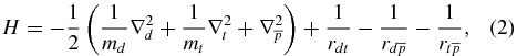
The Hamiltonian of the weakly bound Coulomb three-body systems, equation (2), can be reduced to the sum of the two separated Hamiltonians, i.e. H = Hi + Ho, where the Hamiltonian Hi of the central (or compact) subsystem  and Ho is the Hamiltonian of the outermost particle. For the
  ion, these two Hamiltonians are (in proton-atomic units)

and

The interaction potential  in the Hamiltonian Ho, equation (4), is the short-range potential which is, in fact, a polarization potential. This polarization potential acts between the positively charged deuterium nucleus (electric charge equals +1) and the neutral
  quasi-atom. In this two-body picture, the deuterium nucleus produces 'sufficiently large' polarization of the
  quasi-atom. The interaction between the d+ ion and the polarized
  quasi-atom leads to the formation of the weakly bound state in the
  ion. The boundness of such an ion can accurately be evaluated with the use of perturbation theory (see below). Note also that the actual three-particle potential
  in the
  ion is the difference between the attractive and repulsive Coulomb two-body potentials. All terms in such a potential which have non-zero long-range asymptotics compensate each other. Therefore, at large distances between the central cluster
  and the deuterium nucleus d+ such a potential is almost equal to zero. This allows one to reduce the original, very complex, three-body problem to the interaction of the central, two-body cluster and one deuterium nucleus, i.e. to the two-body problem. Briefly, we can say that the deuterium nucleus produces the electric polarization of the central cluster. If such a polarization is relatively large, then one (or even a few) bound state arises which is stable against dissociation.
The Schrödinger equation HΨ = E · Ψ with the Hamiltonian given by equation (3) is solved exactly and gives us the hydrogen-like wavefunctions  of the two-body quasi-atom
  (or
(or  ). Then, by using these hydrogenic wavefunctions we can compute the expectation value of the Ho operator, equation (4), which is an operator with respect to the (Cartesian) coordinates of the deuterium nucleus d. The origin of the Cartesian coordinates of the deuterium nucleus coincides with the centre of mass of the
  quasi-atom. The kinetic energy of the deuterium nucleus in equation (4) does not change, if we assume that all wavefunctions
  (bound-state wavefunctions) have the unit norm. The expectation value of the sum of the two Coulomb potentials in equation (4) can be replaced by some effective potential V(rd), which in the first-order approximations is the central potential, i.e. V(rd) = V(rd). The explicit form of this effective potential can be obtained with the use of the perturbation theory. This problem is considered in the following section. It is clear that such a picture is only an approximation, since we have ignored a number of additional factors, e.g., contribution from the hydrogenic wavefunctions of the continuous spectrum. Nevertheless, the overall accuracy of this model is surprisingly high and it is still often used for many three-body systems with unit charges.
3. Polarization potential
As shown above, by using the short-range polarization potential in equation (4), one can reduce the analysis of the original three-body Coulomb system with unit charges to the two 'equivalent' two-body problems, equations (3) and (4). In reality, such an 'equivalent' replacement is very difficult to complete, since there are many relations between the explicit form(s) of the model two-body potential in equation (4) and its properties which can be observed in actual, three-body experiments. For instance, as follows from the general theory of the two-body bound states in the non-relativistic potential field, one finds for the total number N(ℓ) of bound states with the angular momentum ℓ

where the central potential V(r) is the polarization potential mentioned above. For the  ion, we have ℓ = 0 and the mass m in the Bargmann inequality, equation (5) (see, e.g., [5] and references therein), is the mass of the deuterium nucleus. A slightly more complicated analysis indicates that the mass m in equation (5) must be chosen as the reduced mass of the deuterium d and
  quasi-atom. Finally, for the
  ion, one finds from equation (5) (in proton-atomic units) that

Note that all particle masses in the  ion are comparable to each other. Therefore, the distribution of the electric charge density in this ion is spherically symmetric (or almost spherically symmetric). The first-order correction upon the charge–dipole interaction between the deuterium nucleus d+ and the
  system is zero, since the spatial distribution of the electric charge in the central
  cluster is spherically symmetric. The second-order perturbation theory leads to the following general form for the interaction V(r) potential between the deuterium nucleus d+ and the neutral quasi-atom
  in the
  ion
ion
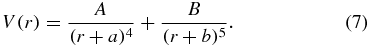
The four constants A, a, B and b in this potential must be in agreement with the prediction which follows from equation (6) and with other experimental data obtained, e.g., from the scattering of the deuterium nucleus at the  system (at different energies). In addition, the two-body system with the interaction potential V(r) must have the same (or almost the same) bound-state properties as the
  ion.
ion.
It should be mentioned that the two-body polarization potential V(r), equation (7), carefully reconstructed with the use of the known scattering data and bound-state properties of the  ion is of some interest in a large number of applications. For instance, the total number of bound states and their approximate geometrical and dynamical properties can be obtained with the use of such a potential. On the other hand, such a potential is only an approximation to the actual three-body potential. Therefore, it is hard to expect that all bound-state properties of the
  ion determined with the model two-body potential will be in good numerical agreement with the actual properties.
4. Variational calculations
In general, the highly accurate computations of weakly bound states in Coulomb three-body systems with unit charges are difficult to perform. The main reason for this is obvious, since all traditional variational expansions contain 'pieces' which describe contributions of fragments from the unbound spectra of two-body systems. In actual computations, this leads to a very slow convergence rate at large dimensions, i.e. when a large number(s) of basis functions N are used in the computations. Traditionally, the highly accurate variational computations of bound states in Coulomb three-body systems with unit charges are performed with the use of the exponential variational expansion in perimetric/relative coordinates. The explicit form of such an expansion for S(L = 0)-states is
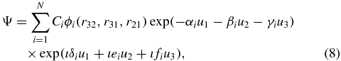
where Ci are the linear (or variational) parameters, αi, βi, γi, δi, ei and fi are the nonlinear parameters and ı is the imaginary unit. The function ϕi(r32, r31, r21) is the polynomial (usually quaratic) function of the three relative coordinates rij. The coefficients of this function are fixed and never varied in calculations. The notations u1, u2 and u3 in equation (8) are the three perimetric coordinates:  . It can be shown that three perimetric coordinates are independent of each other and each of them varies between 0 and +∞.
The variational expansion, equation (8), provides extremely high accuracy in the bound-state computations of arbitrary three-body systems (for more discussions, see, e.g., [6]). For highly accurate calculations of the ground state in the  ion, we can assume that all nonlinear parameters δi, ei, fi equal zero identically, i.e. δi = 0, ei = 0, fi = 0 for i = 1, ..., N. This means that all varied nonlinear parameters in the trial wavefunction, equation (8), are real. This allows one to re-write the formula, equation (8), to the form

which is called the exponential variational expansion in the relative coordinates r32, r31 and r21. In general, the total energy of the ground state of the  ion uniformly depends upon the total number of basis functions N, equation (9), used in the calculations.
Now, the phenomenon of slow convergence at large dimensions can be illustrated with the use of the asymptotic formula for the E(N) dependence

at large N. The formula, equation (10), includes the four parameters E(∞), A1, A2 and δ. The asymptotic energy E(∞) is the improved total energy which is closer to the 'exact' answer than the computed E(Ni) values. For bound states in the Coulomb three-body systems with unit charges, which are not weakly bound, the parameter δ in equation (10) does not change noticeably with N. For weakly bound states in such systems, the parameter δ at large N becomes N-dependent. In many actual cases it decreases when N increases.
To perform numerical calculations in this work, we have used another approach developed in our papers [6]. In that approach, all actual nonlinear parameters of the method (usually 28–40 nonlinear parameters) are carefully optimized at some relatively large dimension, e.g., for N = 1800 and for N = 2200. Then, the total number of basis functions is increased to N = 3500–3840. The optimized values of the nonlinear parameters are not changed during this (last) step. This simple method allows one to obtain results which are significantly more accurate than it is possible to achieve by using old-fashioned numerical procedures with the same numbers of basis functions. Finally, by using our highly accurate wavefunctions, we can determine the expectation values of various bound-state properties. This problem is discussed in the following section.
5. Bound-state properties
The total energy and some other bound-state properties of the  ion can be found in tables 1 and 2. Table 1 contains the total bound-state energies E and the expectation values of all three interparticle delta functions 〈δ(r12)〉, 〈δ(r13)〉, 〈δ(r23)〉 determined in proton-atomic units ℏ = 1, e = 1 and mp = 1. Table 2 includes some other expectation values of the bound-state properties of this ion. These bound-state properties are determined as the expectation values of the corresponding operators, e.g. for the operator
  we write its expectation value X:
where  , n = −2, 1, 2, 3, 4,
  , etc. Here and below, we use the cyclic notations (i, j, k) = (1, 2, 3) which are very convenient for three-body systems. Note that all distances in the
  ion are Mp ≈ 1836 times shorter than the electron-nuclear distances in regular hydrogen atom and hydrogen ion. This means that the distances between the antiproton and tritium/deuterium nuclei in the ground state of the
  ion are ≈2.5–2.6 × 10⁻¹² cm. Briefly, these distances are only ≈20–30 times larger than the corresponding nucleon–nucleon distances in the light few-nucleon nuclei, e.g., in the 3H, 3He and 4He nuclei. This indicates clearly that strong interactions between deuteron, triton and antiproton can contribute significantly to the structure and properties of the bound states in the
  ion. In particular, such a contribution will be large for all properties which include the interparticle delta functions, i.e. δ(rij) values.
Table 1. The convergence of the total energies E and expectation values of the two-particle delta functions for the ground (bound) S(L = 0)-state of the  ion (in proton-atomic units). N is the total number used in the calculations.
| N | E |  |
 |
〈δdt〉 |
|---|---|---|---|---|
| 3300 | −0.381 190 899 643 549 799 44 | 1.035 725 171 596 × 10−1 | 2.650 209 027 68 × 10−2 | 1.971 948 57 × 10−4 |
| 3500 | −0.381 190 899 643 549 803 19 | 1.035 725 171 777 × 10−1 | 2.650 209 025 81 × 10−2 | 1.971 948 65 × 10−4 |
| 3700 | −0.381 190 899 643 549 805 74 | 1.035 725 171 405 × 10−1 | 2.650 209 034 62 × 10−2 | 1.971 948 53 × 10−4 |
| 3840 | −0.381 190 899 643 549 807 25 | 1.035 725 171 481 × 10−1 | 2.650 209 025 13 × 10−2 | 1.971 948 57 × 10−4 |
Table 2. Some bound-state properties of the ground (bound) S(L = 0)-state of the  ion (in proton-atomic units). Particle 1 means deuteron, 2 designates triton, while 3 stands for the antiproton.
| 〈X〉 | (ij) = (32) | (ij) = (31) | (ij) = (21) |
|---|---|---|---|
 |
0.645 258 498 0114 | 0.326 582 953 2244 | 0.209 459 651 948 64 |
| 〈(rikrjk)−1〉 | 0.090 672 197 685 358 | 0.138 335 036 005 26 | 0.173 272 319 919 26 |
 |
0.894 094 641 294 119 | 0.289 502 249 538 164 | 0.063 535 944 062 8808 |
| 〈rij〉 | 2.535 959 239 261 | 5.822 464 028 824 | 6.533 299 013 7423 |
 |
9.369 595 134 746 | 52.356 018 182 35 | 57.621 835 007 682 |
 |
46.657 103 625 69 | 645.749 573 6644 | 676.623 423 785 91 |
 |
294.499 048 4287 | 10 212.706 155 51 | 10 290.298 340 574 |
| τjk | 0.765 842 051 886 31 | 0.340 629 349 170 79 | 0.076 678 419 0714 |
| Fa | 0.084 729 933 577 141 | 0.055 940 481 744 87 | 1.217 745 967 × 10−4 |
| νij | −0.749 606 693 8104 | −0.666 556 443 418 27 | 1.198 635 268 4990 |
| νbij | −0.749 606 690 1228 | −0.666 556 352 630 91 | 1.198 636 672 4385 |
 |
0.069 022 844 172 409 | 0.224 408 939 089 96 | 0.271 702 370 101 33 |
| 〈pi · pj〉 | 0.006 716 068 397 607 | 0.010 606 500 838 45 | 0.012 940 402 539 131 |
| 〈rik · rjk〉 | 50.304 129 027 643 17 | 7.317 705 980 038 39 | 2.051 889 154 707 72 |
 |
−0.410 397 756 7344 | −1.813 210 288 2933 | 0.027 479 444 734 55 |
aThe values of f, 〈(r12r13r23)−1〉 and 〈δ123〉, respectively. bThe exact values of the two-body cusps.
The quality of the computed delta functions δ(rij) can be checked by comparing the computed and predicted values of the corresponding cusp values νij which are defined by the following relations:
where (ij) = (ji) = (12), (13), (23). For few-body systems interacting by the Coulomb and Yukawa-type forces, the numerical values of νij can be predicted and they are not equal zero identically. In particular, for the Coulomb three-body system one finds

where qi and qj are the electric charges and mi and mj are the masses of the particles.
By using any two of the three interparticle delta functions, we can define the three-particle delta function δ123 = δ(rij) · δ(rik). The 〈δ123〉 expectation value is equal to the probability to detect all three particles at one spatial 'non-relativistic' point, i.e. inside of the volume  , where
  is the fine-structure constant, while
  is the Bohr radius. This expectation value plays an important role for some systems, e.g., it is used to predict the one-photon annihilation in the Ps− ion. Formally, by using the three-particle delta function δ123 one can try to construct the three-particle cusp operator ν123, which is equal to the product of the three-particle delta function δ123 and a second-order (partial) derivative
  . However, as follows from the general theory [7], the expectation value of such an operator is infinite for an arbitrary Coulomb three-body system.
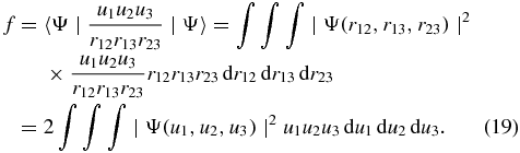
The expectation values of the spatial momenta  are defined as follows:
This integral is reduced to the form of the one-dimensional integral of the product of the one-particle density matrix and  . To simplify the following transformations below, we shall restrict ourselves to the consideration of the bound S(L = 0)-states only. In this case, the wavefunction Ψ is the function of the three scalar interparticle coordinates r12, r13 and r23 only, i.e. Ψ = Ψ(r12, r13, r23). Therefore, we can define the one-particle density matrix

and write the following formula for the  expectation value:

The idea of this method of 'spatial moments' developed in the middle of the 1960s was simple and transparent. Indeed, if we can determine a sufficient number of 'spatial moments', then we can reconstruct, in principle, all three one-particle density matrices ρ(r12), ρ(r13) and ρ(r23). In turn, this will lead us to useful conclusions about the spatial distributions of the two and three particles in the system. However, this idea has never been applied to reconstruct the actual density matrices. Furthermore, since the middle of the 1960s we can approximate the wavefunction of any three-body system to a very high numerical accuracy. By using these wavefunctions, we can determine all spatial momenta to extremely high accuracy (see table 2). However, a few questions about the spatial momenta still remain unanswered for three-body systems. The most interesting question is related to the 'singular momenta', i.e. to the  expectation values with m = −3, −4, −5, .... These expectation values are singular, but their principal and regular parts are needed in some problems, e.g., the values
  are used to evaluate the lowest order QED correction (or Araki–Sucher correction) for Coulomb two-electron atoms and ions (see, e.g., [8] and references therein). Table 2 contains the expectation values of the regular part of the
  expectation value which is designated as
  . These expectation values are related to the corresponding principal parts (
 ) by the following relations (see, e.g., [8] and references therein)
  .
.
Table 2 also contains expectation values which are used to measure various interparticle correlations in three-body systems. The spatial interparticle correlations are evaluated with the use of the three cosine functions τ:
where a · b means the scalar product of the two vectors (a and b), rij = rji, but rij = −rji, since rij = ri − rj. The sum of the three τjk values always exceeds unity, i.e. it can be written in the form

where the f-value is
In some earlier works, the expectation values of the three scalar products rij · rik were proposed to be used to describe spatial interparticle correlations in the three-body systems. Note that the three interparticle vectors rij, rik and rkj always form a triangle. Therefore, we can write

In other words, the expectation values of all three scalar products rij · rik can be expressed from the known  values. This means that these scalar products are not independent properties. An analogous situation can be found for the three scalar products pi · pj of each two single-particle momenta. It follows from the conservation of the total momentum P and its three components (P)i. Indeed, in the centre-of-mass system we can write P = p1 + p2 + p3 = 0. From here, one finds three following identities:

The same identities can be written for the corresponding expectation values. Therefore, the three expectation values of the scalar products pi · pj are uniformly related to the single particle 'kinetic energies'  and cannot be used to describe dynamical correlations between three point particles as independent values.
6. Annihilation and fusion rates
In reality, the three-body  ion is not stable, since it decays either by the proton–antiproton annihilation (at rest) or by the nuclear (d, t)-fusion. Note that the proton–antiproton annihilation in the
  ion proceeds as the tritium–antiproton annihilation or deuterium–antiproton annihilation. In general, the proton–antiproton (or triton–antiproton and deuteron–antiproton) annihilation can proceed with the use of many dozens of reaction channels (see, e.g. [9] and references therein), e.g.,


where π0, π± and K0 are the neutral and charged pions and kaons, respectively. The energy released during the antiproton annihilation is usually around hundreds and even thousands of MeV [9] (this depends upon the annihilation channel).
The reaction of nuclear fusion takes the form

where the antiproton  plays the role of a particle 'catalyzator' which simply brings the two positive particles closer to each other. Formally, the distance between the nuclei of deuterium and tritium is mp ≈ 1836.15 times shorter than in the DT+ molecular ion and ≈ 8.880 times shorter than in the ground state of the muonic molecular ion dtμ. This allows one to evaluate the rate of the (d,t)-nuclear fusion. The approximate value is ≈1 × 10¹³ − 2.5 × 10¹³ s−1. The inverse value gives the approximate lifetime τf of the
  ion against nuclear (d, t)-fusion (τf ≈ 4 × 10⁻¹⁴ − 1 × 10⁻¹³ s). This result is based on the quasi-classical approximation which provides a reasonable accuracy for muonic molecular ions, but can be very approximate for the
  ion. Note also that the probability of formation of the bound, two-body
  He system (also called the
  -system) after such a reaction (catalyzator poisoning) in the
  ion is relatively large (≈ 5% according to our approximate evaluations).
Analogous evaluation of the lifetime of the  ion against antiproton annihilation is significantly more complicated. Currently, both the tritium–antiproton and deuterium–antiproton annihilations at small and very small energies of the colliding particles are not well-studied phenomena. In particular, there are some deviations between the experimental data and theoretical predictions based on different theoretical models (see, e.g., [10–12] and references therein). However, the main problem for low-energy analysis is related with the fact that currently there is no experimental data below 38 MeV/c (the incident moment of the antiproton). Very likely, at small energies there are large differences between annihilation rates obtained for the triplet and singlet states of proton–antiproton pairs. Moreover, the role of antiproton annihilation at neutron(s) at small energies can be evaluated only approximately (see discussion below). It makes any realistic evaluation of the tritium–antiproton and deuterium–antiproton annihilation rates at small/zero energies of the colliding particles almost impossible.
Nevertheless, a few predictions for the ground state in the  ion can be made. Indeed, by using our expectation values of the interparticle delta functions determined for the ground state of the
  ion (see table 1), we can evaluate the relative contributions of the antiproton annihilation at the triton and deuteron nuclei, respectively. Indeed, for the antiproton annihilation rates (Γ) at the deuteron and/or triton, we can write the following formulas:

where the notations  stand for the proton, antiproton and neutron, respectively. From here, one finds

where  is the ratio of the corresponding 'basic' annihilation rates (the rates of the neutron–antiproton and proton–antiproton annihilation at zero interparticle distances). As follows from the results of numerous experiments with heavy antiprotonic atoms ([13] and references therein), the ratio x is close to unity. If ξ = 1, then from equation (26) one finds that for the ground state in the
  ion
ion  . It is extremely interesting to evaluate the actual ratio ξ for the
  ion by performing direct experiments. This will give us important information about the antiproton–neutron annihilation at rest. Also, it follows from table 1 for the
  ion, that the antiproton annihilation rate at the triton is ≈5.862 13 times more likely than annihilation at the deuteron (if ξ = 1). It is clear that experiments with the
  ion can be used for accurate measurements of the ξ ratio at small/zero energies of the colliding particles.
7. Hyperfine structure
The hyperfine structure of the  ion is of great experimental interest, since the magnetic moments of the proton and antiproton are equal to each other by their absolute values, but have opposite signs. Note also that all three particles in the
  ion have non-zero magnetic moments (or spins). Therefore, we can expect that the hyperfine structure of the ground state of the
  ion will be sufficiently rich. Moreover, such a structure and the corresponding hyperfine structure splittings can easily be observed in modern experiments. However, the determined values of the hyperfine splittings of the
  allows us to understand a large number of interesting details related to the long-range asymptotics of the strong interparticle interactions.
For the bound S(L = 0)-state in the  ion, the hyperfine structure is determined by solving the eigenvalue problem for the Hamiltonian (ΔH)h.s. which is responsible for the spin–spin (or hyperfine) interactions. The general formula for such a hyperfine Hamiltonian (ΔH)h.s. in the case of the
  ion is written as the sum of the three following terms. Each of these terms is proportional to the product of the factor
  and the expectation value of the corresponding (interparticle) delta function. The third (additional) factor contains the corresponding g-factors (or gyromagnetic ratios) and scalar product of the two spin vectors. For instance, for the pdμ ion this formula takes the form (in atomic units ℏ = 1, e = 1, me = 1) (see, e.g., [4])
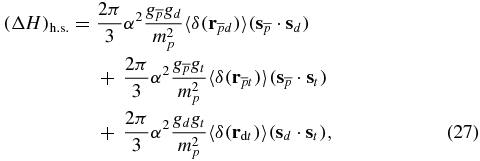
where  is the fine structure constant and
  is the proton mass. Note also that the presence of the common factor
  in all three terms in equation (27) indicates clearly that the proton-atomic units mentioned above are more appropriate for this problem. Nevertheless, below we shall continue to use the usual atomic units ℏ = 1, e = 1 and me = 1. To recalculate the expectation values of the δ-functions from proton-atomic to atomic units one needs to use the factor
  . The expression for (ΔH)h.s., equation (27), is, in fact, an operator in the total spin space which has the dimension (2sp + 1)(2sd + 1)(2st + 1) = 12. In our calculations, we have used the following numerical values for the constants and factors in equation (27): α = 7.297 352 586 × 10−3 and
  . The g-factors for the antiproton, deuteron and triton are determined from the formulas:
  and
and  , where
  and Ia are the corresponding magnetic moments and spins of the particle a. For the triton, deuteron and antiproton, we have
  and
and  , while the magnetic moments of these particles (in nuclear magnetons) are
  and
and  .
.
The hyperfine structure and hyperfine structure splittings of the ground state of the  ion can be found in table 3. Traditionally, these values are expressed in megahertz, or MHz. To recalculate our results from atomic units to MHz, we used the conversion factor 6.579 683 920 61 × 109 MHz au−1 [14]. As follows from table 3, the hyperfine structure of the
  ion includes 12 levels which are separated into the four following groups: (1) the group of five spin states with J = 2, (2) the upper group of three states with J = 1, (3) one state with J = 0 and (4) the lower group of three states with J = 1. The energy differences between these four groups of states are 1.112 524 269 × 108 MHz, 6.853 155 051 × 109 MHz and 5.977 402 022 × 107 MHz. These values can be measured quite accurately by using a modern experimental technique developed to measure atomic hyperfine splittings.
Table 3. The levels of the hyperfine structure  and hyperfine structure splittings Δ of the ground bound S(L = 0) state of the
  ion (in MHz).
| J |
Δ | |
|---|---|---|
 |
2.364 225 7710 × 109 | – |
 |
2.252 973 3441 × 109 | 1.112 524 269 × 108 |
 |
−4.600 181 7067 × 109 | 6.853 155 051 × 109 |
 |
−4.659 955 7269 × 109 | 5.977 402 022 × 107 |
Note again that such a hyperfine structure corresponds to the three-body  ion with the pure Coulomb interaction potentials between particles. In reality, corrections to the strong interactions between particles will change the expectation values of all interparticle delta functions. Therefore, we can expect some changes in the hyperfine structure and hyperfine structure splittings. Such corrections to the hyperfine structure splitting of the
  ion will be the goal of our next study.
8. Conclusion
We have determined the total energy and some bound-state properties of the weakly bound (ground) S(L = 0)-state in the  ion. It is shown that this weakly bound state has a 'two-body' cluster structure, which is represented as the motion of the deuterium nucleus d+ in the central field of the 'central'
  cluster. The interaction between the deuterium nucleus d+ and the two-body
  cluster is the regular dipole–charge interaction, which is often called and considered as the polarization potential. The use of the two-body cluster model and approximate reconstruction of the polarization potential allows one to evaluate qualitatively many bound-state properties of the
  ion. In highly accurate calculations of the ground state of the
  ion performed for this study, we have used our advanced optimization procedure developed in [6] and later improved for large dimensions. This strategy works perfectly for all Coulomb three-body systems, including weakly bound and cluster systems.
A number of bound-state properties of the  ion have been determined to a very high numerical accuracy with the use of our bound-state wavefunctions. In particular, by using the expectation values of the delta functions, we have investigated the hyperfine structure of the ground S(L = 0)-state in the
  ion. In this ion there are 12 levels of hyperfine structure which are separated into four different groups. The energy differences between these groups of states are Δ12 = 1.112 524 269 × 108 MHz, Δ23 = 6.853 155 051 × 109 MHz and Δ34 = 5.977 402 022 × 107 MHz. These values are called the hyperfine structure splittings. The obtained values of the hyperfine structure splittings must be compared with the corresponding experimental values.
Another interesting question for this ion is related to a direct comparison of the rates of the (d, t)-nuclear fusion and rates of the antiproton annihilation at the deuteron and triton, respectively. These problems have solutions which are very sensitive to the contribution from strong interparticle interactions. Therefore, the comparison of the future experimental results and theoretical predictions will lead us to a large number of important conclusions about long-range asymptotics of the strong interactions. Currently, we have developed a number of effective numerical methods for such computations. Moreover, as follows from the results of the first calculations performed with the use of 'realistic' interparticle potentials (Coulomb potential plus term which describes strong interactions), we can say that the contributions from the antiproton–triton and antiproton–deuteron strong interactions play the leading role. Analogous contribution from the deuteron–triton realistic potential is significantly smaller. Therefore, to make accurate predictions for the ground state of the  ion we need to know the interaction potential between the antiproton and triton and deuteron, respectively. The contribution from the triton–deuteron strong interaction is also important, but it is not crucial. In general, the accurate reconstruction of the potential of strong interactions requires a detailed knowledge of all its scalar, spin–orbital (L · S) and tensor components. To reconstruct such a potential for each pair of interacting particles, one needs to know a large amount of scattering data [15] and additional information about all bound two-body states.