Calculation of self-field coefficients for 2D magnetostatic systems

From a physical standpoint, the demagnetizing field ${{\overset{\scriptscriptstyle\rightharpoonup}{H}}_{{\rm m}}}$ is a magnetic field within a specimen of a given material that is generated by the presence of induced or permanent magnetic dipole moments in the material. Also, the magnetization vector $\overset{\scriptscriptstyle\rightharpoonup}{M}$ represents the density of these dipole moments averaged over the volume of a cell. According to Maxwell's equations for magnetostatic fields [1], ${{\overset{\scriptscriptstyle\rightharpoonup}{H}}_{{\rm m}}}$ and $\overset{\scriptscriptstyle\rightharpoonup}{M}$ must satisfy

$$\begin{eqnarray}&&\vec{\nabla }\cdot {{\overset{\scriptscriptstyle\rightharpoonup}{H}}_{{\rm m}}}=-\vec{\nabla }\cdot \overset{\scriptscriptstyle\rightharpoonup}{M},\end{eqnarray} \tag{ 1 }$$

$$\begin{eqnarray}&&\vec{\nabla }\times {{\overset{\scriptscriptstyle\rightharpoonup}{H}}_{{\rm m}}}=\overset{\scriptscriptstyle\rightharpoonup}{0}.\end{eqnarray} \tag{ 2 }$$

Consequently, one can transform the above set of PDEs into Poisson's equation and in turn, solve the latter using appropriate boundary conditions. Moreover, in this case, it is possible to obtain an integral solution for ${{\overset{\scriptscriptstyle\rightharpoonup}{H}}_{{\rm m}}}$ (which involves $\overset{\scriptscriptstyle\rightharpoonup}{M}$ in its integrand) using the Green's function method [2]. However, since the magnetization is not always known, certain textbooks introduce the notion of a demagnetizing field by considering that the problem at hand is such that $\overset{\scriptscriptstyle\rightharpoonup}{M}$ is uniform within the magnetic region [3, 4]. Nevertheless, this remains true under the following assumptions [5]: (1) the material has a constant magnetic susceptibility; (2) an ellipsoidal geometry is considered, which involves spheres, disks and long cylinders as limiting cases and (3) the specimen is subject to a uniform external magnetic field. In effect, the resulting integral expression leads to the definition of the coefficients of the demagnetizing tensor; these types of coefficients are also sometimes referred to as demagnetizing factors [6, 7] or demagnetization factors [3, 4]. It is noteworthy to mention that the representation of ${{\overset{\scriptscriptstyle\rightharpoonup}{H}}_{{\rm m}}}$ under an integral form has the remarkable property of inherently satisfying the boundary conditions of the problem. In fact, this is one of the main reasons that make this form of solution so appealing.

Evaluating the tensor's coefficients is by no means a recent topic of discussion and theoretical values for them are well documented in the literature [6, 7]. Also, numerical methods such as the volume integral equation method calculate these quantities using generalized polygonal elements for 2D systems and right triangular or rectangular prismatic elements for 3D ones [8, 9]. In any case, certain difficulties arise when calculating self-terms of the demagnetizing tensor for which the observation point is located inside the magnetic medium. More precisely, these complications are related to a discontinuity within the integration region. Thus, some authors [1, 10] refer to the work given in [8] for proof but surprisingly, the latter never gives a satisfactory explanation. In effect, this lack of clarity motivated the current paper which is aimed to rigorously explain the mathematical derivation of self-terms as well as provide a general method for their calculation. As it will be shown, in order to remain consistent with the Green's function method used to obtain the integral formulation of the coefficients, one must employ a calculation scheme based on specific integral transformations. Note that, to keep the formalism as simple as possible, the proof will only be presented for 2D magnetostatic cases but its structure pertains to many other situations given the fact that discontinuous integrands commonly arise in physics (e.g. integral solutions of PDEs which use a Green's function).

Let ${{\vec{r}}_{{\rm f}}}$ and ${{\vec{r}}_{{\rm s}}}$ represent the field and source points of a 2D magnetostatic system, respectively, as these vectors are assumed to be mutually independent. More precisely, in the context of this study, a 2D system refers to a magnetic object in a 3D space for which the cross section and all pertinent physical quantities do not change along a particular direction (i.e. a translation invariant system). In this work, the translation invariant axis will be taken along z and so the integral form of the demagnetizing field ${{\overset{\scriptscriptstyle\rightharpoonup}{H}}_{{\rm m}}}$ can be obtained using the methodology given in [1], thus

$$\begin{eqnarray}&&{{\overset{\scriptscriptstyle\rightharpoonup}{H}}_{{\rm m}}}({{\vec{r}}_{{\rm f}}})=\mathop \iint \limits_{S} \;\frac{2(\vec{M}({{{\vec{r}}}_{{\rm s}}})\cdot \vec{r}){\mkern 1mu} \vec{r}-\| {\mkern 1mu} \vec{r}{{{\mkern 1mu} }\| ^{2}}\vec{M}({{{\vec{r}}}_{{\rm s}}})}{2\pi \| {\mkern 1mu} \vec{r}{{{\mkern 1mu} }\| ^{4}}}\;{\rm d}{{x}_{{\rm s}}}{\rm d}{{y}_{{\rm s}}},\end{eqnarray} \tag{ 3 }$$

where S represents an arbitrary 2D region. Moreover, the change of variables $\vec{r}={{\vec{r}}_{{\rm s}}}-{{\vec{r}}_{{\rm f}}}$ has been considered in order to simplify the notation and $\| {\mkern 1mu} \vec{r}{\mkern 1mu}\|$ is the magnitude of the $\vec{r}$ vector. Therefore, under the assumptions given in section 1 [5], S is an ellipse and in turn, one can consider that $\vec{M}={{M}_{x}}\vec{i}+{{M}_{y}}\vec{j}$ is uniform within the magnetic medium and so the above expression becomes

$$\begin{eqnarray}&&{{H}_{{\rm m}x}}({{\vec{r}}_{{\rm f}}})=-\left( {{N}_{xx}}({{{\vec{r}}}_{{\rm f}}}){\mkern 1mu} {{M}_{x}}+{{N}_{xy}}({{{\vec{r}}}_{{\rm f}}}){\mkern 1mu} {{M}_{y}} \right),\end{eqnarray} \tag{ 4 }$$

$$\begin{eqnarray}&&{{H}_{{\rm m}y}}({{\vec{r}}_{{\rm f}}})=-\left( {{N}_{yx}}({{{\vec{r}}}_{{\rm f}}}){\mkern 1mu} {{M}_{x}}+{{N}_{yy}}({{{\vec{r}}}_{{\rm f}}}){\mkern 1mu} {{M}_{y}} \right).\end{eqnarray} \tag{ 5 }$$

Consequently, according to (3)–(5), the coefficients of the demagnetizing tensor are given by

$$\begin{eqnarray}&&{{N}_{xx}}=\frac{1}{2\pi }\;\mathop \iint \limits_{S} \;\frac{{{y}^{2}}-{{x}^{2}}}{{{\left( {{x}^{2}}+{{y}^{2}} \right)}^{2}}}\;{\rm d}{{x}_{{\rm s}}}{\rm d}{{y}_{{\rm s}}},\end{eqnarray} \tag{ 6 }$$

$$\begin{eqnarray}&&{{N}_{xy}}=\frac{1}{2\pi }\;\mathop \iint \limits_{S} \;\frac{-2xy}{{{\left( {{x}^{2}}+{{y}^{2}} \right)}^{2}}}\;{\rm d}{{x}_{{\rm s}}}{\rm d}{{y}_{{\rm s}}},\end{eqnarray} \tag{ 7 }$$

$$\begin{eqnarray}&&{{N}_{yx}}={{N}_{xy}},\end{eqnarray} \tag{ 8 }$$

$$\begin{eqnarray}&&{{N}_{yy}}=-{{N}_{xx}},\end{eqnarray} \tag{ 9 }$$

where the variables $x={{x}_{{\rm s}}}-{{x}_{{\rm f}}}$ and $y={{y}_{{\rm s}}}-{{y}_{{\rm f}}}$ are defined as the components of $\vec{r}$. Note that self-terms are coefficients for which ${{\vec{r}}_{{\rm f}}}\in S$ or in other words, when ${{\vec{r}}_{{\rm s}}}={{\vec{r}}_{{\rm f}}}\leftrightarrow x=y=0$ somewhere within the integration region. Also, it is noteworthy to mention that a complex representation of (6)–(9) is possible as discussed in [9] and [11]. However, in order to keep the approach as transparent as possible, the proposed formalism is developed in real space. Although as stated above, an elliptical shape is necessary for $\vec{M}$ to be independent of position, the method to be discussed for performing the integrals on the right-hand-sides of (6) and (7) is valid for quite general shapes. Therefore, the integrands of (6) and (7) can be rewritten using the following expressions

$$\begin{eqnarray}&&\frac{{{y}^{2}}-{{x}^{2}}}{{{\left( {{x}^{2}}+{{y}^{2}} \right)}^{2}}}=\frac{\partial }{\partial {{x}_{s}}}\left[ \frac{x}{{{x}^{2}}+{{y}^{2}}} \right]=-\frac{\partial }{\partial {{y}_{s}}}\left[ \frac{y}{{{x}^{2}}+{{y}^{2}}} \right],\end{eqnarray} \tag{ 10 }$$

$$\begin{eqnarray}&&\frac{-2xy}{{{\left( {{x}^{2}}+{{y}^{2}} \right)}^{2}}}=\frac{\partial }{\partial {{x}_{s}}}\left[ \frac{y}{{{x}^{2}}+{{y}^{2}}} \right]=\frac{\partial }{\partial {{y}_{s}}}\left[ \frac{x}{{{x}^{2}}+{{y}^{2}}} \right].\end{eqnarray} \tag{ 11 }$$

In order to apply these results, it is useful to consider two general transformations [12] for the integrals described by expressions (6) and (7). Firstly, S is said to be a type I region (figure 1(a)) if it is bounded by

$$\begin{eqnarray}&&{{S}_{{\rm I}}}=\left\{ ({{x}_{{\rm s}}},{{y}_{{\rm s}}})|a\leqslant {{x}_{{\rm s}}}\leqslant b,\;{{g}_{1}}({{x}_{{\rm s}}})\leqslant {{y}_{{\rm s}}}\leqslant {{g}_{2}}({{x}_{{\rm s}}}) \right\},\end{eqnarray} \tag{ 12 }$$

with ${{g}_{1}}$ and ${{g}_{2}}$ representing continuous functions in the interval ${{x}_{{\rm s}}}\in \left[ a,b \right]$. In this case, one can transform a double integral into a line integral using

$$\begin{eqnarray}&&\mathop \iint \limits_{S} \frac{\partial P}{\partial {{y}_{{\rm s}}}}{\rm d}{{x}_{{\rm s}}}{\rm d}{{y}_{{\rm s}}}=-\mathop \oint \limits_{\zeta } P\;{\rm d}{{x}_{{\rm s}}},\end{eqnarray} \tag{ 13 }$$

where ζ is a positively oriented [12], piecewise smooth, simple closed path which lies in a plane and contours S. Furthermore, $P({{x}_{{\rm s}}},{{y}_{{\rm s}}})$ is a scalar function that has continuous partial derivatives in an open region of ${{\Re }^{2}}$ containing S.

Zoom In Zoom Out Reset image size

Secondly, S is said to be a type II region (figure 1(b)) if it is bounded by

$$\begin{eqnarray}&&{{S}_{{\rm II}}}=\left\{ ({{x}_{{\rm s}}},{{y}_{{\rm s}}})|c\leqslant {{y}_{{\rm s}}}\leqslant d,\;{{h}_{1}}({{y}_{{\rm s}}})\leqslant {{x}_{{\rm s}}}\leqslant {{h}_{2}}({{y}_{{\rm s}}}) \right\},\end{eqnarray} \tag{ 14 }$$

with h₁ and h₂ representing continuous functions in the interval ${{y}_{{\rm s}}}\in \left[ c,d \right]$. Consequently, one can write the following equation

$$\begin{eqnarray}&&\mathop \iint \limits_{S} \frac{\partial Q}{\partial {{x}_{{\rm s}}}}\;{\rm d}{{x}_{{\rm s}}}{\rm d}{{y}_{{\rm s}}}=\mathop \oint \limits_{\zeta } Q\;{\rm d}{{y}_{{\rm s}}},\end{eqnarray} \tag{ 15 }$$

where the scalar function $Q\left( {{x}_{{\rm s}}},{{y}_{{\rm s}}} \right)$ has continuous partial derivatives in an open region of ${{\Re }^{2}}$ which contains S. Thus, expressions (6)–(9) can be rewritten as

$$\begin{eqnarray}&&N_{xx}^{({\rm I})}=-N_{yy}^{({\rm I})}=\frac{1}{2\pi }\mathop \oint \limits_{\zeta } \frac{y}{{{x}^{2}}+{{y}^{2}}}{\rm d}{{x}_{{\rm s}}},\end{eqnarray} \tag{ 16 }$$

$$\begin{eqnarray}&&N_{xy}^{({\rm I})}=N_{yx}^{({\rm I})}=-\frac{1}{2\pi }\mathop \oint \limits_{\zeta } \frac{x}{{{x}^{2}}+{{y}^{2}}}{\rm d}{{x}_{{\rm s}}},\end{eqnarray} \tag{ 17 }$$

$$\begin{eqnarray}&&N_{xx}^{({\rm II})}=-N_{yy}^{(I{\rm I})}=\frac{1}{2\pi }\mathop \oint \limits_{\zeta } \frac{x}{{{x}^{2}}+{{y}^{2}}}{\rm d}{{y}_{{\rm s}}},\end{eqnarray} \tag{ 18 }$$

$$\begin{eqnarray}&&N_{xy}^{({\rm II})}=N_{yx}^{({\rm II})}=\frac{1}{2\pi }\mathop \oint \limits_{\zeta } \frac{y}{{{x}^{2}}+{{y}^{2}}}{\rm d}{{y}_{{\rm s}}}.\end{eqnarray} \tag{ 19 }$$

Here, the superscripts (I) and (II) indicate the type of transformation to be used for each case. When S can be considered as either a type I or a type II region, it is said to be a type III region. For example, in the case of an ellipse centered at ${{\vec{r}}_{0}}={{x}_{0}}\vec{i}+{{y}_{0}}\vec{j}$ with its semi-major axis A and semi-minor axis B taken along the x and y axes, respectively, a type I region is defined following expression (12) with ${{x}_{0}}-A\leqslant {{x}_{{\rm s}}}\leqslant {{x}_{0}}+A$, ${{g}_{1}}({{x}_{{\rm s}}})={{y}_{0}}-B\sqrt{1-{{\left( \left( {{x}_{{\rm s}}}-{{x}_{0}} \right)/A \right)}^{2}}}$ and ${{g}_{2}}({{x}_{{\rm s}}})={{y}_{0}}+B\sqrt{1-{{\left( \left( {{x}_{{\rm s}}}-{{x}_{0}} \right)/A \right)}^{2}}}$. Moreover, according to expression (14), this ellipse can be defined as a type II region using ${{y}_{0}}-B\leqslant {{y}_{{\rm s}}}\leqslant {{y}_{0}}+B$, ${{h}_{1}}({{y}_{{\rm s}}})={{x}_{0}}-A\sqrt{1-{{\left( \left( {{y}_{{\rm s}}}-{{y}_{0}} \right)/B \right)}^{2}}}$ and ${{h}_{2}}({{y}_{{\rm s}}})={{x}_{0}}+A\sqrt{1-{{\left( \left( {{y}_{{\rm s}}}-{{y}_{0}} \right)/B \right)}^{2}}}$. Thus, in this case, S corresponds to a type III region and so, according to expressions (16)–(19), both transformations must lead to the same result, hence

$$\begin{eqnarray}&&N_{xx}^{({\rm I})}-N_{xx}^{({\rm II})}=0\leftrightarrow \frac{1}{2\pi }\mathop \oint \limits_{\zeta } \left[ \frac{y\;\vec{i}}{{{x}^{2}}+{{y}^{2}}}-\frac{x\;\vec{j}}{{{x}^{2}}+{{y}^{2}}} \right]\cdot {\rm d}{{\vec{r}}_{{\rm s}}}=0,\end{eqnarray} \tag{ 20 }$$

$$\begin{eqnarray}&&N_{xy}^{({\rm I})}-N_{xy}^{({\rm II})}=0\leftrightarrow -\frac{1}{2\pi }\mathop \oint \limits_{\zeta } \left[ \frac{x\;\vec{i}}{{{x}^{2}}+{{y}^{2}}}+\frac{y\;\vec{j}}{{{x}^{2}}+{{y}^{2}}} \right]\cdot {\rm d}{{\vec{r}}_{{\rm s}}}=0.\end{eqnarray} \tag{ 21 }$$

In order to validate these expressions for any given geometry, it is useful to note that a line integral is independent of the path ζ when the curl of its integrand is $\vec{0}$, which in this case is satisfied by

$$\begin{eqnarray}&&{{\vec{\nabla }}_{{\rm s}}}\times \left[ \frac{y\;\vec{i}}{{{x}^{2}}+{{y}^{2}}}-\frac{x\;\vec{j}}{{{x}^{2}}+{{y}^{2}}} \right]=\vec{0},\end{eqnarray} \tag{ 22 }$$

$$\begin{eqnarray}&&{{\vec{\nabla }}_{{\rm s}}}\times \left[ \frac{x\;\vec{i}}{{{x}^{2}}+{{y}^{2}}}+\frac{y\;\vec{j}}{{{x}^{2}}+{{y}^{2}}} \right]=\vec{0}.\end{eqnarray} \tag{ 23 }$$

It is important to mention that this formalism is independent of the geometry and it is always valid for any kind of physical problem which generates integrals similar to equations (6) and (7). Furthermore, using expressions (20)–(23), one concludes that the coefficients for type I and II transformations are always equivalent if S is a type III region. However, this reasoning is incomplete: expressions (13) and (15) require the integrands of (6)–(9) to be continuous in an open region of ${{\Re }^{2}}$ containing S, but this continuity was never verified. In fact, upon a closer examination of these quantities, one finds that the integrands of all the coefficients are discontinuous at ${{\vec{r}}_{{\rm s}}}={{\vec{r}}_{{\rm f}}}$. 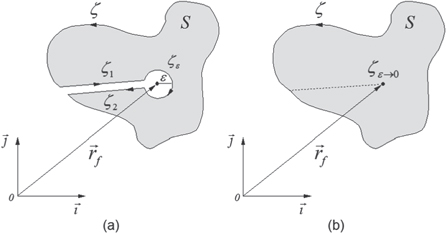In other words, self-terms will not necessarily yield reliable results when applying type I and II transformations. To get around this problem, consider an arbitrary 2D magnetic region S (as shown in figure 2) with a uniform magnetization and containing a circular sub-path ζ_ε centered at ${{\vec{r}}_{{\rm f}}}$ with ε representing the radius of this path. Moreover, as shown in figure 2(a), one must introduce two additional sub-paths ζ₁ and ζ₂ in order for the resulting path to be closed.

Zoom In Zoom Out Reset image size

Thus, substituting ζ for ζ + ζ_ε + ζ₁ + ζ₂ and setting ε → 0 leads to a more appropriate form for expressions (20) and (21). However, in this case, ζ₁ and ζ₂ have opposite directions and therefore both these sub-paths cancel out and can be omitted from the representation (figure 2(b)). Consequently, the aforementioned equations can be rewritten as

$$\begin{eqnarray}&&N_{xx}^{({\rm I})}-N_{xx}^{({\rm II})}=\frac{{{\delta }_{S}}\left( {{{\vec{r}}}_{{\rm f}}} \right)}{2\pi }\mathop{{\rm lim} }\limits_{\varepsilon \to 0}\mathop \oint \limits_{\zeta } \left[ -\frac{y\;\vec{i}}{{{x}^{2}}+{{y}^{2}}}+\frac{x\;\vec{j}}{{{x}^{2}}+{{y}^{2}}} \right]\cdot {\rm d}{{\vec{r}}_{{\rm s}}},\end{eqnarray} \tag{ 24 }$$

$$\begin{eqnarray}&&N_{xy}^{({\rm I})}-N_{xy}^{({\rm II})}=\frac{{{\delta }_{S}}({{{\vec{r}}}_{{\rm f}}})}{2\pi }\mathop{{\rm lim} }\limits_{\varepsilon \to 0}\mathop \oint \limits_{\zeta } \left[ \frac{x\;\vec{i}}{{{x}^{2}}+{{y}^{2}}}+\frac{y\;\vec{j}}{{{x}^{2}}+{{y}^{2}}} \right]\cdot {\rm d}{{\vec{r}}_{{\rm s}}},\end{eqnarray} \tag{ 25 }$$

where ${{\delta }_{S}}({{\vec{r}}_{{\rm f}}})$ represents a Kronecker delta which is worth 1 for self-terms $({{\vec{r}}_{{\rm f}\,}}\in S)$ and 0 otherwise $({{\vec{r}}_{{\rm f}}}\notin S)$. Now, the circular sub-path can be represented by the change of variables $x=\varepsilon {\rm cos} \theta$ and $y=\varepsilon {\rm sin} \theta ,$ where $\theta \in \left[ 0,\ \;2\pi \right[$ is the angle between the vectors $\vec{i}$ and $\vec{r}$. Taking the limit of the integrals performed along ζ_ε yields

$$\begin{eqnarray}&&\mathop{{\rm lim} }\limits_{\varepsilon \to 0}{{\oint }_{{{\zeta }_{}}}}\frac{y}{{{x}^{2}}+{{y}^{2}}}{\rm d}{{x}_{{\rm s}}}=\int \limits_{2\pi }^{0} -{{{\rm sin} }^{2}}\theta \;{\rm d}\theta =\pi ,\end{eqnarray} \tag{ 26 }$$

$$\begin{eqnarray}&&\mathop{{\rm lim} }\limits_{\varepsilon \to 0}{{\oint }_{{{\zeta }_{}}}}\frac{x}{{{x}^{2}}+{{y}^{2}}}{\rm d}{{y}_{{\rm s}}}=\int \limits_{2\pi }^{0} {{{\rm cos} }^{2}}\theta \;{\rm d}\theta =-\pi ,\end{eqnarray} \tag{ 27 }$$

$$\begin{eqnarray}&&\mathop{{\rm lim} }\limits_{\varepsilon \to 0}{{\oint }_{{{\zeta }_{}}}}\frac{x}{{{x}^{2}}+{{y}^{2}}}{\rm d}{{x}_{{\rm s}}}=\int \limits_{2\pi }^{0} -{\rm sin} \theta {\rm cos} \theta \;{\rm d}\theta =0,\end{eqnarray} \tag{ 28 }$$

$$\begin{eqnarray}&&\mathop{{\rm lim} }\limits_{\varepsilon \to 0}{{\oint }_{{{\zeta }_{}}}}\frac{y}{{{x}^{2}}+{{y}^{2}}}{\rm d}{{y}_{{\rm s}}}=\int \limits_{2\pi }^{0} {\rm sin} \theta {\rm cos} \theta \;{\rm d}\theta =0.\end{eqnarray} \tag{ 29 }$$

Note that the integration of θ is taken clockwise from 2π to 0 since by definition, all paths are positively oriented (see figure 2(a)). Finally, combining (24)–(29) leads to the following expressions

$$\begin{eqnarray}&&N_{xx}^{({\rm I})}-N_{xx}^{({\rm II})}=N_{yy}^{({\rm II})}-N_{yy}^{({\rm I})}=-{{\delta }_{S}}({{\vec{r}}_{{\rm f}}}),\end{eqnarray} \tag{ 30 }$$

$$\begin{eqnarray}&&N_{xy}^{({\rm I})}-N_{xy}^{({\rm II})}=N_{yx}^{({\rm I})}-N_{yx}^{({\rm II})}=0.\end{eqnarray} \tag{ 31 }$$

From the above results, it can be concluded that for a type III region, type I and II transformations are always equivalent for N_xy and N_yx, but are not for self-field coefficients of N_xx and N_yy. To make some sense out of the latter result, it is insightful to examine the mathematical formalism which led up to the integral formulation of the coefficients. To begin with, according to the Green's function method [2], 2D magnetostatic systems have a Green's function G defined as

$$\begin{eqnarray}G({{\vec{r}}_{{\rm s}}},{{\vec{r}}_{{\rm f}}})=\left\{ \begin{array}{ccccccccccccccc} \frac{1}{2\pi }{\rm ln} \;(R*) & {\rm for} & \| \vec{r}\| \lt R*, \\ \frac{1}{2\pi }{\rm ln} \;\left( \sqrt{{{x}^{2}}+{{y}^{2}}} \right) & {\rm for} & \| \vec{r}\| \geqslant R*, \\ \end{array} \right.\end{eqnarray} \tag{ 32 }$$

with R* representing a fixed cutoff radius and $\| \;\vec{r}\;\| =\sqrt{{{x}^{2}}+{{y}^{2}}}\geqslant 0$. Note that both terms constituting G are directly proportional to one of the linearly independent isotropic solutions obtained when solving Laplace's equation in polar coordinates. Thus, one can always set R* → 0 so that the method at hand requires the function G to satisfy

$$\begin{eqnarray}&&\nabla _{{\rm s}}^{2}G=\mathop{{\rm lim} }\limits_{{{R}^{*}}\to 0}\delta \left(\| \vec{r}\| -{{R}^{*}} \right)=\delta \left(\| {\mkern 1mu} \vec{r} \| \right),\end{eqnarray} \tag{ 33 }$$

where $\nabla _{{\rm s}}^{2}$ is the Laplace operator with respect to ${{\vec{r}}_{{\rm s}}}$ and $\delta \left( \| \;\vec{r}\;{\mkern 1mu} \| \right)$ is the Dirac delta function (i.e. associated to a continuous function). As for the coefficients N_xx and N_yy, they can be derived from G according to

$$\begin{eqnarray}&&{{N}_{xx}}=\mathop \iint \limits_{S} \frac{{{\partial }^{2}}}{\partial x_{{\rm s}}^{2}}\left[ \frac{1}{2\pi }{\rm ln} \left( \sqrt{{{x}^{2}}+{{y}^{2}}} \right) \right]{\rm d}{{x}_{{\rm s}}}{\rm d}{{y}_{{\rm s}}},\end{eqnarray} \tag{ 34 }$$

$$\begin{eqnarray}&&{{N}_{yy}}=\mathop \iint \limits_{S} \frac{{{\partial }^{2}}}{\partial y_{{\rm s}}^{2}}\left[ \frac{1}{2\pi }{\rm ln} \left( \sqrt{{{x}^{2}}+{{y}^{2}}} \right) \right]{\rm d}{{x}_{{\rm s}}}{\rm d}{{y}_{{\rm s}}}.\end{eqnarray} \tag{ 35 }$$

In fact, adding these expressions leads to

$$\begin{eqnarray}&&{{N}_{xx}}+{{N}_{yy}}=\mathop \iint \limits_{S} \nabla _{{\rm s}}^{2}\left[ \frac{1}{2\pi }{\rm ln} \left( \sqrt{{{x}^{2}}+{{y}^{2}}} \right) \right]{\rm d}{{x}_{{\rm s}}}{\rm d}{{y}_{{\rm s}}}=0,\end{eqnarray} \tag{ 36 }$$

which is identical to expression (9). Note that the integrand of (36) cancels out because it satisfies by definition Laplace's equation. However, what this result does not explicitly show is that for self-terms, equation (33) implies that

$$\begin{eqnarray}&&{{N}_{xx}}+{{N}_{yy}}=\mathop \iint \limits_{S} \delta \left(\| \vec{r}\| \right){\rm d}{{x}_{{\rm s}}}{\rm d}{{y}_{{\rm s}}}={{\delta }_{S}}({{\vec{r}}_{{\rm f}}}).\end{eqnarray} \tag{ 37 }$$

Therefore, this expression yields N_xx + N_yy = 1 for self-terms, a classic result that most authors refer to when studying the demagnetizing field [3, 5–10]. Thus, returning to expressions (16), (18) and (30), one finds that the only way to remain consistent with the above equation is to write

$$\begin{eqnarray}&&N_{xx}^{({\rm II})}+N_{yy}^{({\rm I})}={{\delta }_{S}}({{\vec{r}}_{{\rm f}}}).\end{eqnarray} \tag{ 38 }$$

This expression represents a crucial result not found in the open literature. That is to say, to properly model self-terms of 2D magnetostatic systems, N_xx must absolutely be evaluated with a type II transformation and N_yy with a type I transformation. Moreover, according to expressions (17), (19) and (31), the coefficients N_xy and N_yx can be evaluated using both types of transformations. In fact, proceeding any other way leads to mathematical inconsistencies with the Green's function method used to obtain the integral formulation of the coefficients and in turn, yields incorrect self-terms. Note that the above result is useful for anyone trying to evaluate the coefficients of the demagnetizing tensor, be it for theoretical or numerical purposes. For instance, teachers who wish to demonstrate to their students that N_xx + N_yy = 1 without using (37) will be hard pressed to do so taking into account (6) and (9), since these expressions lead to N_xx + N_yy = 0 ≠ 1; the only way to get around this problem is by presenting the coefficients using their line integral forms and remembering that N_yy and N_xx must absolutely be evaluated using a type I and II transformation, respectively. It is important to mention that, according to our knowledge, this is the first work that permits the analytical calculation of the demagnetizing coefficients as given in [6] using a 2D approach.

The integrals representing 2D coefficients of the magnetostatic demagnetizing tensor can, under a set of specific mathematical criteria, be rewritten as line integrals using type I or II transformations. However, for self-terms $({{\vec{r}}_{{\rm f}}}\in S)$, the integrands of the coefficients are discontinuous at ${{\vec{r}}_{{\rm s}}}={{\vec{r}}_{{\rm f}}}$ which means that the aforementioned transformations are not reliable in this case. Thus, the generalization of both transformations for self-terms was achieved by appropriately contouring the singularity. Also, in order to remain consistent with the Green's function method used to obtain the integral formulation of the coefficients, it was found that N_xx must absolutely be evaluated with a type II transformation and N_yy with a type I transformation, a detail not proved nor mentioned in the open literature. Seeing how 2D systems were considered all throughout this document, there still remains the generalization of 3D self-terms to be formally proven. Work is currently underway to formulate this proof.

The work presented in this paper was possible due to the financial support of the Natural Sciences and Engineering Research Council of Canada (NSERC) under the Discovery Research Grant RGPIN 41929.