


ABSTRACT
We extensively reanalyze the effects of a long-lived, negatively charged massive particle, X−, on big bang nucleosynthesis (BBN). The BBN model with an X− particle was originally motivated by the discrepancy between the 6, 7Li abundances predicted in the standard BBN model and those inferred from observations of metal-poor stars. In this model, 7Be is destroyed via the recombination with an X− particle followed by radiative proton capture. We calculate precise rates for the radiative recombinations of 7Be, 7Li, 9Be, and 4He with X−. In nonresonant rates, we take into account respective partial waves of scattering states and respective bound states. The finite sizes of nuclear charge distributions cause deviations in wave functions from those of point-charge nuclei. For a heavy X− mass, mX ≳ 100 GeV, the d-wave → 2P transition is most important for 7Li and 7, 9Be, unlike recombination with electrons. Our new nonresonant rate of the 7Be recombination for mX = 1000 GeV is more than six times larger than the existing rate. Moreover, we suggest a new important reaction for 9Be production: the recombination of 7Li and X− followed by deuteron capture. We derive binding energies of X nuclei along with reaction rates and Q values. We then calculate BBN and find that the amount of 7Be destruction depends significantly on the charge distribution of 7Be. Finally, updated constraints on the initial abundance and the lifetime of the X− are derived in the context of revised upper limits to the primordial 6Li abundance. Parameter regions for the solution to the 7Li problem and the primordial 9Be abundances are revised.
Export citation and abstract BibTeX RIS
1. INTRODUCTION
Standard big bang nucleosynthesis (SBBN) is an important probe of the early universe. This model explains the primordial light element abundances inferred from astronomical observations except for the 7Li abundance. Additional nonstandard effects during big bang nucleosynthesis (BBN) may be required to explain the 7Li discrepancy. However, such models are strongly constrained from the consistency in the other elemental abundances. In this paper, we re-examine in detail one intriguing solution to the 7Li problem, which is due to a late-decaying, negatively charged particle (possibly the stau as the next to lightest supersymmetric particle) denoted as X−. In previous work (Kusakabe et al. 2008), we showed that both a decrease in 7Li and an increase in 6Li abundances are possible in this model. Recently, however, the primordial 6Li abundance has been revised downward (Lind et al. 2013), and there is now only an upper limit. Hence, it is necessary to re-evaluate the X− solution in light of these new measurements. We show that this remains a viable model for 7Li reduction without violating the new 6Li upper limit.
1.1. Primordial Li Observations
The primordial lithium abundance is inferred from spectroscopic measurements of metal-poor stars (MPSs). These stars have a roughly constant abundance ratio, 7Li/H =(1 − 2) × 10−10, as a function of metallicity (Spite & Spite 1982; Ryan et al. 2000; Meléndez & Ramírez 2004; Asplund et al. 2006; Bonifacio et al. 2007; Shi et al. 2007; Aoki et al. 2009; González Hernández et al. 2009; Sbordone et al. 2010; Monaco et al. 2010, 2012; Mucciarelli et al. 2012; Aoki et al. 2012; Aoki 2012). The SBBN model, however, predicts a value that is higher by about a factor of three to four (e.g., 7Li/H = 5.24 × 10⁻¹⁰ Coc et al. 2012) than the observational value when one uses the baryon-to-photon ratio determined in the ΛCDM model from an analysis of the power spectrum of the cosmic microwave background (CMB) radiation from the Wilkinson Microwave Anisotropy Probe (WMAP; Larson et al. 2011; Hinshaw et al. 2013) or the Planck data (Coc et al. 2013). This discrepancy suggests the need for a mechanism to reduce the 7Li abundance during or after BBN. Astrophysical processes such as rotationally induced mixing (Pinsonneault et al. 1999, 2002) and the combination of atomic and turbulent diffusion (Richard et al. 2005; Korn et al. 2007; Lind et al. 2009) might have reduced the 7Li abundance in stellar atmospheres, although this possibility is constrained by the very narrow dispersion in observed Li abundances.
In previous work, the 6Li/7Li isotopic ratios for MPSs have also been measured and 6Li detections have been reported for the halo turnoff star HD 84937 (Smith et al. 1993, 1998; Cayrel et al. 1999), the two Galactic disk stars, HD 68284 and HD 130551 (Nissen et al. 1999), and other stars (Asplund et al. 2006; Inoue et al. 2005; Asplund & Meléndez 2008; García Pérez et al. 2009; Steffen et al. 2010, 2012). A large 6Li abundance of 6Li/H ∼6 × 10⁻¹² was suggested (Asplund et al. 2006). That abundance is ∼1000 times higher than the SBBN prediction and is also significantly higher than the prediction from a standard Galactic cosmic-ray nucleosynthesis model (cf. Prantzos 2006, 2012). It has been noted for some time, however (Smith et al. 2001; Cayrel et al. 2007), that convective motion in stellar atmospheres could cause systematic asymmetries in the observed atomic line profiles and mimic the presence of 6Li (Cayrel et al. 2007). Indeed, in a subsequent detailed analyses, Lind et al. (2013) found that most of the previous 6Li absorption feature could be attributed to a combination of three-dimensional (3D) turbulence and nonlocal thermal equilibrium (NLTE) effects in the model atmosphere. For the present purposes, therefore, we adopt the 2σ upper limit from their G64-12 NLTE model with five parameters corresponding to 6Li/H <9.5 × 10⁻¹².
Abundances of 9Be (Boesgaard et al. 1999; Primas et al. 2000; Tan et al. 2009; Smiljanic et al. 2009; Ito et al. 2009; Rich & Boesgaard 2009) and B (Duncan et al. 1997; Garcia Lopez et al. 1998; Primas et al. 1999; Cunha et al. 2000) in MPSs have also been measured. The observed abundances linearly scale with Fe abundances. The linear relation between abundances of light elements and Fe is expected in Galactic cosmic-ray nucleosynthesis models (Reeves 1970, 1974; Meneguzzi et al. 1971; Prantzos 2012). Any primordial abundances, on the other hand, should be observed as a plateau in abundance at low metallicities as in the case of 7Li. Be and B in the observed MPSs are not expected to be primordial. Nonetheless, primordial abundances of Be and B may be found by future observations. The strongest lower limit on the primordial Be abundance at present is log(Be/H) <−14 which has been derived from an observation of the carbon-enhanced MPS BD+44°493 with an iron abundance [Fe/H] =−3.77 with Subaru/HDS (Ito et al. 2009).
1.2. X− Solution
As one of the solutions to the lithium problem, effects of negatively charged massive particles (CHAMPs or Cahn-Glashow particles) X− (Cahn & Glashow 1981; Dimopoulos et al. 1990; de Rújula et al. 1990) during the BBN epoch have been studied (Pospelov 2007b; Kohri & Takayama 2007; Cyburt et al. 2006; Hamaguchi et al. 2007; Bird et al. 2008; Kusakabe et al. 2007, 2008; Jedamzik 2008a, 2008b; Kamimura et al. 2009, 2010; Pospelov 2007a; Kawasaki et al. 2007, 2008; Jittoh et al. 2007, 2008, 2010; Pospelov et al. 2008; Khlopov & Kouvaris 2008; Bailly et al. 2009; Jedamzik & Pospelov 2009; Kusakabe et al. 2010; Pospelov & Pradler 2010; Kohri et al. 2012; Cyburt et al. 2012; Đapo et al. 2012). Constraints on supersymmetric models have been derived through BBN calculations (Cyburt et al. 2006; Kawasaki et al. 2007, 2008; Jittoh et al. 2007, 2008, 2010; Pradler & Steffen 2008a, 2008b; Bailly et al. 2009). In addition, cosmological effects of fractionally charged massive particles (FCHAMPs) have been studied, although the nucleosynthesis has not yet been studied (Langacker & Steigman 2011).
Such long-lived CHAMPs and FCHAMPs, which are also called heavy stable charged particles, appear in theories beyond the standard model, and have been searched for in collider experiments. Although the particles should leave characteristic tracks corresponding to long times of flight due to small velocities and anomalous energy losses, they have never been detected. The most stringent limit on scalar supersymmetric partner of the tau lepton (stau) has been derived using data collected with the Compact Muon Solenoid detector for pp collisions at the Large Hadron Collider during the 2011 ( TeV, 5.0 fb−1) and 2012 (
 TeV, 18.8 fb−1) data taking periods. The data exclude stau mass below 500 GeV for the direct+indirect production model (Chatrchyan et al. 2013b). The limit on spin 1/2 FCHAMPs that are neutral under SU(3)C and SU(2)L has also been derived from Compact Muon Solenoid searches. It excludes the masses less than 310 GeV for charge number q = 2/3, and masses less than 140 GeV for q = 1/3 (Chatrchyan et al. 2013a).
The X− particles and nuclei A can form new bound atomic systems (AX or X-nuclei) with binding energies ∼O(0.1–1) MeV in the limit that the mass of the X−, mX, is much larger than the nucleon mass (Cahn & Glashow 1981; Kusakabe et al. 2008). The X-nuclei are exotic chemical species with very heavy masses and chemical properties similar to normal atoms and ions. The super-heavy stable (long-lived) particles have been searched for in experiments, and multiple constraints on respective X-nuclei have been derived. The spectroscopy of terrestrial water gives a limit on the number ratio of X/H <10−28–10−29 for mX = 11–1100 GeV (Smith et al. 1982), while that of sea water gives the limits of X/H <4 × 10⁻¹⁷ for mX = 5–1500 GeV (Yamagata et al. 1993) and X/H <6 × 10⁻¹⁵ for mX = 104–107 GeV (Verkerk et al. 1992). Limits on the X-to-nucleon ratio have been derived from analyses of other material: (1) X/N <5 × 10⁻¹² for mX = 102–105 GeV from Na (Dick et al. 1986), (2) X/N <2 × 10⁻¹⁵ for mX ⩽ 105 GeV from C (Turkevich et al. 1984), and (3) X/N <1.5 × 10⁻¹³ for mX ⩽ 105 GeV from Tl (Norman et al. 1989). Furthermore, limits from analyses of H, Li, Be, B, C, O, and F have been derived for mX = 102–104 GeV using commercial gases, lake and deep sea water deuterium, plant 13C, commercial 18O, and reagent grade samples of Li, Be, B, and F (Hemmick et al. 1990).
If the X− particle exits during the BBN epoch, it opens new pathways of atomic and nuclear reactions and affects the resultant nucleosynthesis (Pospelov 2007b; Kohri & Takayama 2007; Cyburt et al. 2006; Hamaguchi et al. 2007; Bird et al. 2008; Kusakabe et al. 2007, 2008; Jedamzik 2008a, 2008b; Kamimura et al. 2009; Pospelov 2007a; Kawasaki et al. 2007; Jittoh et al. 2007, 2008, 2010; Pospelov et al. 2008; Khlopov & Kouvaris 2008; Kawasaki et al. 2008; Bailly et al. 2009; Kamimura et al. 2010; Kusakabe et al. 2010; Pospelov & Pradler 2010; Kohri et al. 2012; Cyburt et al. 2012; Đapo et al. 2012).
As the temperature of the universe decreases, positively charged nuclides gradually become electromagnetically bound to X− particles. Heavier nuclei with larger mass and charge numbers recombine earlier since their binding energies are larger (Cahn & Glashow 1981; Kusakabe et al. 2008). The formation of most X-nuclei proceeds through radiative recombination of nuclides A and X− (Dimopoulos et al. 1990; de Rújula et al. 1990). However, the 7BeX formation also proceeds through the non-radiative 7Be charge exchange reaction between a 7Be3 + ion and an X− (Kusakabe et al. 2013a, 2013b). The recombination of 7Be with X− occurs in a higher temperature environment than that of lighter nuclides. At 7Be recombination, therefore, the thermal abundance of free electrons e− is still very high, and abundant 7Be3 + ions can exist. The charge exchange reaction then only affects the 7Be abundance.
Because of relatively small binding energies, the bound states cannot form until late in the BBN epoch. At low temperatures, the nuclear reactions are already inefficient. Hence, the effect of the X− particles is not large. However, the X− particle can cause efficient production of 6Li (Pospelov 2007b) with the weak destruction of 7Be (Bird et al. 2008; Kusakabe et al. 2007) depending on its abundance and lifetime (Bird et al. 2008; Kusakabe et al. 2008, 2010).
The 6Li abundance can significantly increase through the X−-catalyzed transfer reaction 4HeX(d, X−)6Li (Pospelov 2007b). The cross section of the reaction is six orders of magnitude larger than that of the radiative 4He(d, γ)6Li reaction through which 6Li is produced in the SBBN model (Hamaguchi et al. 2007). Other transfer reactions such as 4HeX(t, X−)7Li, 4HeX(3He,X−)7Be, and 6LiX(p, X−)7Be are also possible (Cyburt et al. 2006). Their rates are, however, not as large as that of the 4HeX(d, X−)6Li since the former reactions involve a Δl = 1 angular momentum transfer and consequently a large hindrance of the nuclear matrix element (Kamimura et al. 2009).
The most important reaction for a reduction of the primordial 7Li abundance8 is the resonant reaction 7BeX(p, γ)8BX through the first atomic excited state of 8BX (Bird et al. 2008) and the atomic ground state (GS) of 8B*(1+,0.770 MeV)X, i.e., an atom consisting of the 1+ nuclear excited state of 8B and an X− (Kusakabe et al. 2007). From a realistic estimate of binding energies for X-nuclei, however, the latter resonance has been found to be an inefficient pathway for 7BeX destruction (Kusakabe et al. 2008).
The 8BeX+p → 9B BX+γ reaction through the 9B
 atomic excited state of 9BX (Kusakabe et al. 2008) produces the A =9 X-nucleus so that it can possibly lead to the production of heavier nuclei. This reaction, however, is not operative because of its large resonance energy (Kusakabe et al. 2008).
The resonant reaction 8BeX(n, X−)9Be through the atomic GS of 9Be*(1/2+, 1.684 MeV)X is another reaction producing nuclei with A = 9 nuclide (Pospelov 2007a). Kamimura et al. (2009), however, adopted a realistic root mean square charge radius for 8Be of 3.39 fm, and found that 9Be*(1/2+, 1.684 MeV)X is not a resonance but a bound state located below the 8BeX+n threshold. A subsequent four-body calculation for the α + α + n + X− system confirmed that the 9Be*(1/2+, 1.684 MeV)X state is located below the threshold (Kamimura et al. 2010). This was also confirmed by Cyburt et al. (2012) using a three-body model. The effect of the resonant reaction is therefore negligible. The detailed BBN calculations of Kusakabe et al. (2008, 2010) precisely incorporate recombination reactions of nuclides and X− particles, nuclear reactions of X-nuclei, and their inverse reactions. These calculations have also included reaction rates estimated in a rigorous quantum few-body model (Hamaguchi et al. 2007; Kamimura et al. 2009). The most realistic calculation (Kusakabe et al. 2010) shows no significant production of 9Be and heavier nuclides.
Reactions of neutral X-nuclei, i.e., pX, dX, and tX, can produce and destroy Li and Be (Jedamzik 2008a, 2008b). The rates for these reactions and the charge-exchange reactions pX(α, p)αX, dX(α, d)αX, and tX(α, t)αX have been calculated in a rigorous quantum few-body model (Kamimura et al. 2009). The cross sections for the charge-exchange reactions are much larger than those of the nuclear reactions so that the neutral X-nuclei pX, dX, and tX are quickly converted to αX before they induce nuclear reactions. The production and destruction of Li and Be is not significantly affected by the presence of neutral X-nuclei (Kamimura et al. 2009). This was confirmed in a detailed nuclear reaction network calculation (Kusakabe et al. 2010). It has been shown in our previous work (Kusakabe et al. 2008, 2010) that concordance with the observational constraints on D, 3He, and 4He is maintained in the parameter region of 7Li reduction.
In this paper, we present an extensive study on effects of a CHAMP, X−, on BBN. First, we study the effects of theoretical uncertainties in the nuclear charge distributions on the binding energies of nuclei and the X−, reaction rates, and BBN. Next, we derive the most precise radiative recombination rates for 7Be, 7Li, 9Be, and 4He with an X−. Finally, we suggest a new reaction for 9Be production, i.e., 7LiX(d, X−)9Be. Based upon our updated BBN calculation, it is found that the amount of 7Be destruction depends significantly upon the assumed charge density for the 7Be nucleus. The most realistic constraints on the initial abundance and the lifetime of the X− are then derived, and the primordial 9Be abundance is also estimated.
In Section 2, models for the nuclear charge density are described. In Section 3, binding energies of the X-nuclei are calculated with both a variational method and the integration of the Sch dinger equation for different charge densities. In Section 4, reaction rates are calculated for the radiative proton capture of reactions 7BeX(p, γ)8BX, and 8BeX(p, γ)9BX. Theoretical uncertainties in the rates due to the assumed charge density shapes are deduced. In Section 5, rates for the radiative recombination of 7Be, 7Li, 9Be, and 4He with X− particles are calculated. Both nonresonant and resonant rates are derived. The difference of the recombination rate for X− particles compared to that for electrons is shown. In Section 6, a new reaction for 9Be production is pointed out. It is the radiative recombination of 7Li and an X− followed by deuteron capture. In Section 7, the rates and Q-values for β-decays and nuclear reactions involving the X− particle are derived. In Section 8, a new reaction network calculation code is explained. In Section 9, we show the evolution of elemental abundances as a function of cosmic temperature and derive the most realistic constraints on the initial abundance and the lifetime of the X−. Parameter regions for the solution to the 7Li problem, and the prediction of primordial 9Be are presented. Section 10 is devoted to a summary and conclusions. In the Appendix, we comment on the electric dipole transitions of X-nuclei which change nuclear and atomic states simultaneously.9
2. NUCLEAR CHARGE DENSITY
We assume that a CHAMP with a single negative charge and spin zero was present during the BBN epoch. We derive general constraints depending on the mass of the X−, i.e., mX. The mass is treated as one parameter. Although the existence of very light CHAMPs is excluded by searches in collider experiments, their existence during the BBN epoch is also considered in this paper. This could occur, for example, if the mass of the X− were time dependent. In order to estimate possible uncertainties in the binding energies of nuclei and X− particles which are associated with the nuclear charge density, we use three different shapes for the charge density. The first is a Woods–Saxon (WS) shape:

where r' is the distance from the center of mass of the nucleus, Ze is the charge of the nucleus, R is the parameter characterizing the nuclear size, a is nuclear surface diffuseness, and CWS is a normalization constant. The CWS value is fixed by the equation of charge conservation,  , and it is given by

For a given value of diffuseness a, R can be constrained so that the parameter set of (a, R) satisfies the root-mean-square (rms) charge radius 〈r2〉C1/2 measured in nuclear experiments.
The potential between an X− and a nucleus A (XA potential) is calculated by folding the Coulomb potential with the charge density:
where  is the position vector from an X− to the center of mass of A,
  is the position vector from the center of mass of A,
  is the displacement vector between the X− and the position, and
  is the charge density of the nucleus. The charge density could be distorted from the density of a normal nucleus by the potential of an X−. The distortion effect, however, is relatively small because of the weak Coulomb potential. Hence, we neglect it in this study. Under the assumption of a WS charge distribution ρWS(r'), the potential reduces to the form
The second charge density adopted in this study is a Gaussian shape described by
where the range parameter is related to the rms charge radius by  . The XA potential is given by
where  is the error function.
The third charge density is a square well given by
where H(x) is the Heaviside step function and the surface radius is related to the rms charge radius by  . The XA potential is then given by
3. BINDING ENERGY
Binding energies and wave functions for bound states of X-nuclei are calculated for four different X-particle masses: mX = 1, 10, 100, and 1000 GeV. We performed both numerical integrations of the Schr dinger equation with RADCAP (Bertulani 2003)10 and variational calculations with the Gaussian expansion method (Hiyama et al. 2003). It was confirmed that binding energies derived with the two methods generally agree with each other to within ∼1 %.
Table 1 shows the adopted experimental rms charge radii, and calculated binding energies of GS X-nuclides for mX = 100 TeV. This mass is chosen as one example in which the X− particle is much heavier than the lighter nuclei. Hence, the reduced mass of the A + X− system is given by μ = mAmX/(mA + mX) → mA, where mA is the mass of nuclide A. The second and the third columns show measured rms charge radii and the associated reference, respectively. Results for three different nuclear charge distributions, i.e., Gaussian (fourth column), homogeneous (fifth column), and WS with three values for the diffuseness parameter a = 0.45 fm (WS45; sixth column), 0.4 fm (WS40; seventh), and 0.35 fm (WS35; eighth), are shown. We have chosen these three values for the diffuseness parameter a since larger a values do not lead to simultaneous solutions of R that reproduce the rms charge radii for all nuclides.
Table 1. Binding Energies of AX (MeV) for mX = 100 TeV
| Nuclei |  (fm) (fm) |
Reference | Gaussian | Homogeneous | WS(0.45 fm) | WS(0.4 fm) | WS(0.35 fm) |
|---|---|---|---|---|---|---|---|
| 1H | 0.875 ± 0.007 | 1 | 0.0250 | 0.0250 | 0.0250 | 0.0250 | 0.0250 |
| 2H | 2.116 ± 0.006 | 2 | 0.0489 | 0.0488 | 0.0489 | 0.0489 | 0.0488 |
| 3H | 1.755 ± 0.086 | 3 | 0.0724 | 0.0724 | 0.0725 | 0.0725 | 0.0724 |
| 3He | 1.959 ± 0.030 | 3 | 0.268 | 0.267 | 0.268 | 0.268 | 0.267 |
| 4He | 1.80 ± 0.04 | 4 | 0.343 | 0.342 | 0.344 | 0.343 | 0.343 |
| 6Li | 2.48 ± 0.03 | 4 | 0.806 | 0.790 | 0.802 | 0.799 | 0.797 |
| 7Li | 2.43 ± 0.02 | 4 | 0.882 | 0.862 | 0.878 | 0.874 | 0.871 |
| 8Li | 2.42 ± 0.02 | 4 | 0.945 | 0.921 | 0.940 | 0.936 | 0.932 |
| 6Be | 2.52 ± 0.02a | 4 | 1.234 | 1.201 | 1.225 | 1.220 | 1.215 |
| 7Be | 2.52 ± 0.02 | 4 | 1.324 | 1.284 | 1.313 | 1.306 | 1.300 |
| 8Be | 2.52 ± 0.02a | 4 | 1.401 | 1.353 | 1.387 | 1.379 | 1.373 |
| 9Be | 2.50 ± 0.01 | 4 | 1.477 | 1.422 | 1.462 | 1.452 | 1.445 |
| 10Be | 2.40 ± 0.02 | 4 | 1.577 | 1.516 | 1.564 | 1.553 | 1.544 |
| 7B | 2.68 ± 0.12b | 5 | 1.752 | 1.684 | 1.726 | 1.717 | 1.709 |
| 8B | 2.68 ± 0.12 | 5 | 1.840 | 1.762 | 1.810 | 1.799 | 1.790 |
| 9B | 2.68 ± 0.12b | 5 | 1.917 | 1.829 | 1.883 | 1.871 | 1.860 |
| 10B | 2.58 ± 0.07 | 6 | 2.036 | 1.939 | 2.004 | 1.989 | 1.976 |
| 11B | 2.58 ± 0.07c | 6 | 2.099 | 1.993 | 2.063 | 2.047 | 2.034 |
| 12B | 2.51 ± 0.02 | 4 | 2.198 | 2.082 | 2.164 | 2.145 | 2.129 |
| 9C | 2.51 ± 0.02d | 4 | 2.554 | 2.428 | 2.517 | 2.496 | 2.479 |
| 10C | 2.51 ± 0.02d | 4 | 2.638 | 2.499 | 2.597 | 2.574 | 2.556 |
| 11C | 2.51 ± 0.02d | 4 | 2.713 | 2.562 | 2.668 | 2.644 | 2.623 |
| 12C | 2.51 ± 0.02 | 4 | 2.780 | 2.618 | 2.731 | 2.705 | 2.683 |
| 8B*a | 2.68 ± 0.12 | 5 | 1.021 | 1.024 | 1.022 | 1.022 | 1.023 |
| 9B*a | 2.68 ± 0.12b | 5 | 1.104 | 1.105 | 1.105 | 1.104 | 1.104 |
Notes. aTaken from 7Be radius. bTaken from 8B radius. cTaken from 10B radius. dTaken from 12C radius. References. (1) Yao et al. 2006; (2) Simon et al. 1981; (3) TUNL Nuclear Data, http://www.tunl.duke.edu/NuclData; (4) Tanihata et al. 1988; (5) Fukuda et al. 1999; (6) Cichocki et al. 1995.
Download table as: ASCIITypeset image
Binding energies of the first atomic excited states, 8B and 9B
 , are also shown since they are important in resonant reactions through the atomic excited states that result in 7BeX destruction and 9BX production. The superscript *a indicates an atomic excited state, which is different from a nuclear excited state indicated by a superscript *. Binding energies for the Gaussian charge distribution are the largest. Those for a homogeneous distribution are the smallest, while those for the WS distribution are intermediate. In addition, with a larger diffuseness parameter, the binding energies are larger. The reason for this ordering of binding energies is as follows. The five cases are arranged as (1) Gaussian, (2) WS with a large a value, (3) an intermediate a value, (4) a small a value, and (5) the homogeneous distribution. These are listed in descending order of nuclear charge density at small radii r. When the charge density at small r is relatively large, the Coulomb potential between A and X− is large. Then, large values for the binding energies are derived. It is noted that in all cases, the amplitudes of the Coulomb potentials are smaller than those for two point-charges. This is because of the finite size of charge distribution of the nucleus A. Binding energies are therefore smaller than those in the Bohr's atomic model.
Table 2 shows calculated binding energies of GS X-nuclides and the first atomic excited states of 8B and 9B
 in the WS40 model for mX = 1 GeV (second column), 10 GeV (third column), 100 GeV (fourth column), and 1000 GeV (fifth column). The WS charge distribution with a diffuseness parameter of a = 0.4 fm is taken as our primary model in this paper. When mX is larger, the reduced mass μ = mAmX/(mA + mX) is larger. Binding energies are then larger. However, the binding energies for mX = 100 GeV and 1000 GeV do not differ from each other since the reduced masses in both cases are already near the limiting value of μ = mAmX/(mA + mX) → mA.
Table 2. Binding Energies of AX for a Woods–Saxon Charge Density with a = 0.40 fm (MeV)
| Nuclei | mX = 1 GeV | 10 GeV | 100 GeV | 1000 GeV |
|---|---|---|---|---|
| 1H | 0.0127 | 0.0228 | 0.0247 | 0.0249 |
| 2H | 0.0173 | 0.0414 | 0.0480 | 0.0488 |
| 3H | 0.0196 | 0.0572 | 0.0706 | 0.0723 |
| 3He | 0.0776 | 0.216 | 0.261 | 0.267 |
| 4He | 0.0830 | 0.263 | 0.333 | 0.342 |
| 6Li | 0.194 | 0.615 | 0.776 | 0.797 |
| 7Li | 0.198 | 0.659 | 0.847 | 0.872 |
| 8Li | 0.201 | 0.693 | 0.904 | 0.932 |
| 6Be | 0.335 | 0.970 | 1.189 | 1.216 |
| 7Be | 0.341 | 1.023 | 1.270 | 1.302 |
| 8Be | 0.346 | 1.066 | 1.340 | 1.375 |
| 9Be | 0.350 | 1.108 | 1.408 | 1.448 |
| 10Be | 0.355 | 1.164 | 1.502 | 1.548 |
| 7B | 0.511 | 1.389 | 1.676 | 1.712 |
| 8B | 0.518 | 1.440 | 1.755 | 1.795 |
| 9B | 0.524 | 1.483 | 1.821 | 1.866 |
| 10B | 0.532 | 1.554 | 1.933 | 1.983 |
| 11B | 0.536 | 1.587 | 1.987 | 2.041 |
| 12B | 0.542 | 1.644 | 2.079 | 2.138 |
| 9C | 0.739 | 2.004 | 2.435 | 2.490 |
| 10C | 0.745 | 2.050 | 2.508 | 2.568 |
| 11C | 0.750 | 2.090 | 2.572 | 2.636 |
| 12C | 0.755 | 2.125 | 2.629 | 2.697 |
| 8B*a | 0.147 | 0.665 | 0.973 | 1.017 |
| 9B*a | 0.149 | 0.703 | 1.047 | 1.099 |
Download table as: ASCIITypeset image
Figure 1 shows binding energies of GS X-nuclides and the first atomic excited states of 8B and 9B
 in the five models of nuclear charge distribution for mX = 100 TeV. As the nuclear mass increases, the nuclear charge number and the reduced mass become larger. Therefore, heavier nuclei generally have larger binding energies. Error bars indicate uncertainties originating from the experimental 1σ error in the rms charge radii.
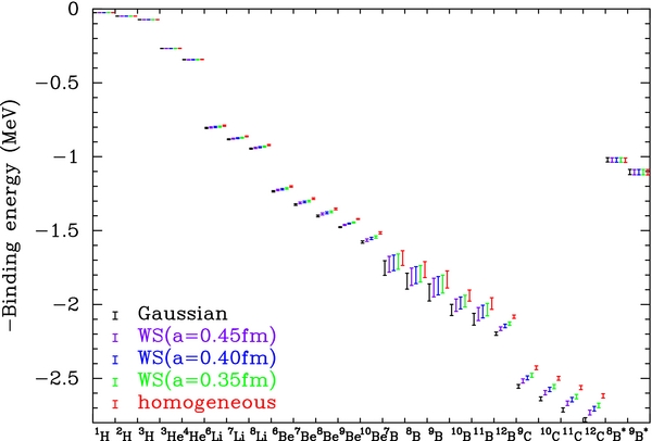
Figure 1. Binding energies of nuclei and X− particles with mX = 100 TeV for different charge distributions. For respective nuclei, calculated results for Gaussian (leftmost lines), Woods–Saxon type with diffuseness parameters a = 0.45 fm (second lines from the left), 0.40 fm (third lines), and 0.35 fm (fourth lines), and a homogeneous well (fifth lines) are shown. Error bars indicate uncertainties determined from uncertainties in the experimental rms charge radii.
Download figure:
Standard image High-resolution imageErrors in binding energies of nuclides up to 4He are small, while those for heavier nuclides can be  (0.1 MeV). However, Q-values for most reactions involving X-nuclei heavier than 4HeX are large, ≳ 1 MeV (e.g., Kusakabe et al. 2008). Effects of errors in binding energies on the rates of forward and inverse reactions are then small. Two exceptions are 7BeX(p, γ)8BX (Q = 0.64 MeV) and 8BeX(p, γ)9BX (Q = 0.33 MeV). These reactions are also exceptional because the resonant components in their reaction rates can be dominant. For the reason described above, we adopted data calculated for the WS40 model, such as nuclear masses, reaction rates, coefficients for reverse reactions, and Q-values. Only data for the reactions 7BeX(p, γ)8BX and 8BeX(p, γ)9BX are calculated for three models of charge distribution, i.e., Gaussian, WS, and homogeneous types.
In the limit that the mass of the X− particle is much larger than that of light nuclides  (1 GeV), reaction rates of the radiative neutron capture are very small. This is because the electric multipole moments approach zero in this limit and the electric matrix elements are very small. This situation is similar to the case of the long-lived, strongly interacting massive particle X0 (Kusakabe et al. 2009). Therefore, we assume that rates of radiative neutron capture reactions are vanishingly small in this study. This is different from the assumption in Kusakabe et al. (2008, 2010).
Figure 2 shows binding energies of GS X-nuclides and the first atomic excited states, 8B and 9B
 , for nuclear charge distribution models of Gaussian (dashed lines), WS40 (solid lines), and homogeneous (dot–dashed lines) as a function of mX. Resonance energies Er are also shown for 8B
 and 9B
 measured relative to the separation channels, 7BeX+p and 8BeX+p. Binding energies are larger when the value of mX is larger, and they approach the asymptotic value in the limit of μ → mA. Maxima are observed in the curves of Er(8B
 ) and Er(9B
 ) at mX ≲ 10 GeV. The resonance energies increase with increasing mX in the mass region of mX ≲ 10 GeV, while they are approximately saturated in the region of mX ≳ 10 GeV. Since rates of the resonant reactions are sensitive to the resonance energies, results of BBN including the existence of X− significantly depend on the mass mX, as described below. Open circles show binding energies of EB(7BeX), EB(8BX), EB(8B
 ), and the resonance energy Er(8B
 ) derived by a quantum many-body calculation for mX = ∞ (Kamimura et al. 2009). The open circles are consistent with calculated values in the Gaussian model.

Figure 2. Binding energies and resonance energies as a function of mX. The upper black lines show resonance energies in the reactions 7BeX(p, γ)8BX and 8BeX(p, γ)9BX. The lower lines show binding energies of 7BeX (black lines), 8BeX (purple lines), 8BX (green lines), 9BX (gray lines), and the first atomic excited states 8B (red lines) and 9B
 (blue lines). Results for different nuclear charge distributions, i.e., Gaussian (dashed lines), Woods–Saxon type with diffuseness parameter a = 0.40 fm (solid lines), and homogeneous well (dot-dashed lines) are drawn. Open circles show energies derived by a quantum many-body calculation (Kamimura et al. 2009) for mX = ∞.
Download figure:
Standard image High-resolution imageFigures 3 and 4 show wave functions of the GS and first atomic excited states of 8B and 9B
 for the case of mX = 1000 GeV with nuclear charge distribution models of Gaussian (dashed lines), WS40 (solid lines), and homogeneous (dot–dashed lines). There are differences between the three lines for the GS of 8BX and 9BX, although they are relatively small. On the other hand, differences are hardly seen for the excited states. Shapes of the charge distribution predominantly affect the Coulomb potentials at small r values. When angular momentum exists, such as in the l = 1 excited states of 8B
 and 9B
 , however, the effect of the centrifugal potential l(l + 1)/2μr2 is significant. The effect of the nuclear charge distribution is therefore most important for GS X-nuclei whose amplitudes of wave functions at small r are larger than those of the excited states. The Gaussian type has the largest Coulomb potential, the WS type has the second largest, and the homogeneous type the smallest. Because of the Coulomb attractive force, the wave functions in the Gaussian model are located in a region of smaller r than those in other models, while those in the homogeneous case are the most extended radially.
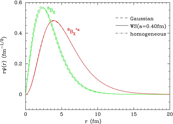
Figure 3. Wave functions for the ground state of 8BX and the first atomic excited state 8B as a function of radius r for mX = 1000 GeV. Lines are drawn for different nuclear charge distributions as labeled, i.e., Gaussian (dashed lines), Woods–Saxon type with diffuseness parameter a = 0.40 fm (solid lines), and a homogeneous well (dot–dashed lines).
Download figure:
Standard image High-resolution image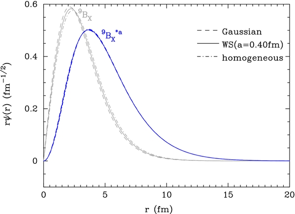
Figure 4. Wave functions for the ground state of 9BX and the first atomic excited state 9B as a function of radius r for mX = 1000 GeV. Lines are drawn for different nuclear charge distributions as labeled, i.e., Gaussian (dashed lines), Woods–Saxon type with diffuseness parameter a = 0.40 fm (solid lines), and a homogeneous well (dot–dashed lines).
Download figure:
Standard image High-resolution image4. RESONANT PROTON CAPTURE REACTIONS
Two important resonant reactions are
where (2P) indicates the atomic 2P state and m(A) and m(AX) are masses of nucleus A and X-nucleus AX, respectively. Resonant rates for these radiative capture reactions can be calculated as follows.
The thermal reaction rate is derived as a function of temperature T by numerically integrating the cross section over a Maxwellian energy distribution,
where E is the center of mass kinetic energy and σ(E) is the reaction cross section as a function of E.
The thermal reaction rate for isolated and narrow resonances is given (Angulo et al. 1999) by
where NA is Avogadro's number, A is the reduced mass in atomic mass units (amu) given by A = A1A2/(A1 + A2) with A1 and A2 the masses of two interacting particles, 1 and 2, in amu, and T9 = T/(109 K) is the temperature in units of 109 K. The parameter ω is a statistical factor defined by
where Ii is the spin of the particle i, J is the spin of the resonance, and δ12 is the Kronecker delta necessary to avoid a double counting of identical particles. The quantity in Equation (11) γ is defined by
where Γi and Γf are the partial widths for the entrance and exit channels, respectively. Γ(Er) is the total width for a resonance with resonance energy Er, γ, MeV is the γ factor in units of MeV, and Er, MeV is the resonance energy in units of MeV.
When ω = 1 as in the reactions considered here and the radiative decay widths of 8B and 9B
 Γγ are much smaller than those for proton emission (as assumed here), the thermal reaction rate is given by
where Γγ, MeV = Γγ/(1 MeV) is the radiative decay width in units of MeV and C is a rate coefficient determined from A and Γγ.
The rate for a spontaneous emission via an electric dipole (E1) transition is given (Blatt & Weisskopf 1991) by
where
is the effective charge with mi and Zi the mass and the charge number of species i = 1 and 2. Eγ is the energy of the emitted photon, Ii is the angular momentum of the initial state, and Mi and Mf are magnetic quantum numbers of initial and final states with μ = Mi − Mf. Ψi and Ψf are wave functions of the initial and final states, respectively, and  is the dipole spherical surface harmonic.
We assume that the nuclear states do not significantly change between 8, 9B and 8, 9BX. For both resonances of 8, 9B
 , the quantity Γγ, MeV is estimated to be

where e1 = e(ZBmX − ZXmB)/(mB + mX) is the effective charge with ZB = 5 and ZX = −1 the charge numbers of 8, 9B and the X−, respectively, and  is the radial matrix element.
Figure 5 shows thermonuclear reaction rates for resonant reactions 7BeX(p, γ)8BX (black lines) and 8BeX(p, γ)9BX (purple lines) as a function of T9 for the case of mX = 1000 GeV. Thick dashed, solid, and dot–dashed lines correspond to Gaussian type, WS40, and homogeneous type nuclear charge distributions, respectively. The thin dashed line corresponds to the reaction rate for 7BeX(p, γ)8BX derived by means of a quantum many-body model calculation for mX = ∞ (Kamimura et al. 2009). Since the resonant reaction rate is proportional to the Boltzmann suppression factor of exp (− Er/T), relatively small differences in resonance energies between different charge distribution cases (Figure 2) can lead to significant differences in the reaction rates.
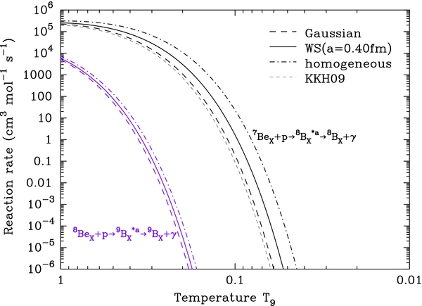
Figure 5. Thermonuclear reaction rates for resonant reactions 7BeX(p, γ)8BX (black lines) and 8BeX(p, γ)9BX (purple lines) as a function of T9 ≡ T/(109 K) for the case of mX = 1000 GeV. Lines are drawn for different nuclear charge distributions as labeled, i.e., Gaussian (thick dashed lines), Woods–Saxon type with diffuseness parameter a = 0.40 fm (solid lines), and a homogeneous well (dot–dashed lines). The thin dashed line shows the reaction rate for 7BeX(p, γ)8BX derived by means of a quantum many-body model for mX = ∞ (Kamimura et al. 2009).
Download figure:
Standard image High-resolution imageTables 3 and 4 show calculated parameters for the resonant reactions 7BeX(p, γ)8BX and 8BeX(p, γ)9BX for the three model charge distributions and with a fixed mass of mX = 1 TeV. The matrix elements, the resonance energies, the energies of emitted photons, the radiative decay widths of the resonances, the rate coefficients, and the reaction Q-values are listed in the second to seventh columns, respectively.
Table 3. Calculated Parameters for 7BeX(p, γ)8BX with mX = 1 TeV
| Model | τif | Er | Eγ | Γγ | C | Q-value |
|---|---|---|---|---|---|---|
| (fm) | (MeV) | (MeV) | (eV) | (106 cm3 mol−1 s−1) | (MeV) | |
| Gaussian | 2.98 | 0.167 | 0.820 | 10.0 | 1.55 | 0.653 |
| homogeneous | 3.18 | 0.124 | 0.740 | 8.43 | 1.30 | 0.615 |
| WS40 | 3.08 | 0.148 | 0.778 | 9.19 | 1.42 | 0.630 |
Download table as: ASCIITypeset image
Table 4. Calculated Parameters for 8BeX(p, γ)9BX with mX = 1 TeV
| Model | τif | Er | Eγ | Γγ | C | Q-value |
|---|---|---|---|---|---|---|
| (fm) | (MeV) | (MeV) | (eV) | (106 cm3 mol−1 s−1) | (MeV) | |
| Gaussian | 2.84 | 0.484 | 0.814 | 8.91 | 1.37 | 0.330 |
| homogeneous | 3.05 | 0.435 | 0.725 | 7.30 | 1.12 | 0.290 |
| WS40 | 2.95 | 0.462 | 0.767 | 8.06 | 1.24 | 0.305 |
Download table as: ASCIITypeset image
The resonance energy, the dipole photon energy, and the reaction Q-value are given by
respectively, where the quantities E(7Be+p) = 0.1375 MeV and E(8Be+p) = −0.1851 MeV are binding energies of 8B and 9B with respect to the energies of the separation channels, respectively.
Tables 5 and 6 show calculated parameters of the resonant reactions 7BeX(p, γ)8BX and 8BeX(p, γ)9BX, respectively, obtained with the WS40 model for mX = 1, 10, 100, and 1000 GeV. The matrix elements, the resonance energies, the energies of emitted photons, the radiative decay widths of resonances, the rate coefficients, and the reaction Q-values are listed in the second to seventh columns, respectively.
Table 5. Calculated Parameters for 7BeX(p, γ)8BX Obtained with the WS40 Model
| mX | τif | Er | Eγ | Γγ | C | Q-value |
|---|---|---|---|---|---|---|
| (GeV) | (fm) | (MeV) | (MeV) | (eV) | (106 cm3 mol−1 s−1) | (MeV) |
| 1 | 9.50 | 0.0568 | 0.372 | 0.838 | 0.154 | 0.315 |
| 10 | 3.87 | 0.220 | 0.775 | 6.29 | 1.05 | 0.555 |
| 100 | 3.16 | 0.160 | 0.782 | 8.88 | 1.39 | 0.622 |
| 1000 | 3.08 | 0.148 | 0.778 | 9.19 | 1.42 | 0.630 |
Download table as: ASCIITypeset image
Table 6. Calculated Parameters for 8BeX(p, γ)9BX Obtained with the WS40 Model
| mX | τif | Er | Eγ | Γγ | C | Q-value |
|---|---|---|---|---|---|---|
| (GeV) | (fm) | (MeV) | (MeV) | (eV) | (106 cm3 mol−1 s−1) | (MeV) |
| 1 | 9.41 | 0.382 | 0.375 | 0.794 | 0.143 | −0.00699 |
| 10 | 3.76 | 0.549 | 0.780 | 5.65 | 0.940 | 0.232 |
| 100 | 3.03 | 0.477 | 0.774 | 7.81 | 1.22 | 0.297 |
| 1000 | 2.95 | 0.462 | 0.767 | 8.06 | 1.24 | 0.305 |
Download table as: ASCIITypeset image
In our BBN calculation, resonant rates for the proton capture reactions are adopted, while the nonresonant rates are taken from Kamimura et al. (2009).
5. RADIATIVE RECOMBINATION WITH X−
5.1. 7Be
5.1.1. Energy Levels
Table 7 shows the binding energies of 7BeX atomic states with main quantum numbers n ranging from one to seven. Since the 7Be nuclear charge distribution has a finite size, the amplitude of the Coulomb potential at small r is less than that for two point-charges. Wave functions at small radii and binding energies of tightly bound states with small n values therefore deviate from those of the Bohr model. Binding energies in the Bohr model are given by  , where α is the fine structure constant. On the other hand, the binding energies of loosely bound states with large n values are similar to those of the Bohr model.
Table 7. Binding Energies of 7BeX Atomic States with Main Quantum Numbers n = 1–7 (keV)
| mX = 1 GeV | l = 0 | l = 1 | l = 2 | l = 3 | l = 4 | l = 5 | l = 6 |
|---|---|---|---|---|---|---|---|
| n = 1 | 341 | ||||||
| n = 2 | 88.7 | 92.3 | |||||
| n = 3 | 40.0 | 41.0 | 41.1 | ||||
| n = 4 | 22.6 | 23.1 | 23.1 | 23.1 | |||
| n = 5 | 14.5 | 14.8 | 14.8 | 14.8 | 14.8 | ||
| n = 6 | 10.1 | 10.3 | 10.3 | 10.3 | 10.3 | 10.3 | |
| n = 7 | 7.45 | 7.54 | 7.54 | 7.54 | 7.54 | 7.54 | 7.54 |
| mX = 10 GeV | l = 0 | l = 1 | l = 2 | l = 3 | l = 4 | l = 5 | l = 6 |
| n = 1 | 1023 | ||||||
| n = 2 | 326 | 409 | |||||
| n = 3 | 158 | 183 | 187 | ||||
| n = 4 | 92.4 | 104 | 105 | 105 | |||
| n = 5 | 60.7 | 66.4 | 67.3 | 67.3 | 67.3 | ||
| n = 6 | 42.9 | 46.2 | 46.8 | 46.8 | 46.8 | 46.8 | |
| n = 7 | 31.9 | 34.0 | 34.4 | 34.4 | 34.4 | 34.4 | 34.4 |
| mX = 100 GeV | l = 0 | l = 1 | l = 2 | l = 3 | l = 4 | l = 5 | l = 6 |
| n = 1 | 1270 | ||||||
| n = 2 | 451 | 603 | |||||
| n = 3 | 226 | 274 | 290 | ||||
| n = 4 | 135 | 156 | 163 | 163 | |||
| n = 5 | 89.7 | 101 | 104 | 105 | 105 | ||
| n = 6 | 63.9 | 70.4 | 72.4 | 72.6 | 72.6 | 72.6 | |
| n = 7 | 47.8 | 51.9 | 53.2 | 53.3 | 53.3 | 53.3 | 53.3 |
| mX = 1000 GeV | l = 0 | l = 1 | l = 2 | l = 3 | l = 4 | l = 5 | l = 6 |
| n = 1 | 1302 | ||||||
| n = 2 | 469 | 632 | |||||
| n = 3 | 236 | 288 | 306 | ||||
| n = 4 | 142 | 164 | 172 | 173 | |||
| n = 5 | 94.3 | 106 | 110 | 111 | 111 | ||
| n = 6 | 67.2 | 74.2 | 76.6 | 76.8 | 76.8 | 76.8 | |
| n = 7 | 50.3 | 54.8 | 56.3 | 56.4 | 56.4 | 56.4 | 56.4 |
Download table as: ASCIITypeset image
5.1.2. 7Be(X−, γ)7BeX Resonant Rate
The resonant rates of the reaction 7Be(X−, γ)7BeX are calculated for mX = 1, 10, 100, and 1000 GeV adopting the WS40 model for the nuclear charge distribution. The normalization of the total charge leads to a radius parameter, R = 2.63 fm. Radiative decay widths for E1 transitions are calculated taking into account the change of the E1 effective charge as a function of mX.
In general, the recombination can efficiently proceed via resonant reactions through atomic states  composed of a nuclear excited state 7Z* and an X− (Bird et al. 2008). In these reactions, the resonances radiatively decay to lower energy states of
  , 7Z*X,
  , and 7ZX that have larger binding energies. Once bound states are produced in the reaction, subsequent transitions via radiative decays to lower energy states occur quickly. Finally, the GS 7ZX is produced after atomic states are converted to the atomic GS, and the nuclear excited state 7Z* inside the atomic states is converted to the nuclear GS (Bird et al. 2008).
Table 8 shows calculated parameters of important transitions related to the reaction 7Be(X−, γ)7BeX for mX = 1, 10, 100, and 1000 GeV. There are an infinite number of atomic states of 7Be , composed of the first nuclear excited state 7Be*[≡ 7Be*(0.429 MeV, 1/2−)] and an X−. Among them states that satisfy EB ≲ 0.4291 MeV are important resonances in the recombination. We take into account atomic resonances with binding energies of 0.23 MeV ⩽EB ⩽ 0.43 MeV. They are the 1S state for mX = 1 GeV, the 2S and the 2P states for mX = 10 GeV, and the 3S, 3P, and 3D states for mX = 100 GeV and 1000 GeV. The transitions, matrix elements, radiative decay widths of the resonance, and resonance energies are listed in the second to fifth columns, respectively.
Table 8. Calculated Parameters for 7Be(X−, γ)7BeX in the WS40 Model
| mX | Transition | τif | Γγ | Er |
|---|---|---|---|---|
| (GeV) | (fm) | (eV) | (MeV) | |
| 1 | 7Be (1S)→ 7BeX(1S) (1S)→ 7BeX(1S) |
⋅⋅⋅ | 0.00343a | 0.0881 |
| 10 | 7Be (2P)→ 7Be (2P)→ 7Be (1S) (1S) |
4.29 | 2.80 | 0.0198 |
| 100 | 7Be (3D)→ 7Be (3D)→ 7Be (2P) (2P) |
6.04 | 1.64 | 0.140 |
| 100 | 7Be (3P)→ 7Be (3P)→ 7Be (2S) (2S) |
8.09 | 0.438 | 0.155 |
| 100 | 7Be (3P)→ 7Be (3P)→ 7Be (1S) (1S) |
0.738 | 0.653 | 0.155 |
| 1000 | 7Be (3D)→ 7Be (3D)→ 7Be (2P) (2P) |
5.80 | 1.84 | 0.123 |
| 1000 | 7Be (3P)→ 7Be (3P)→ 7Be (2S) (2S) |
7.84 | 0.481 | 0.141 |
| 1000 | 7Be (3P)→ 7Be (3P)→ 7Be (1S) (1S) |
0.693 | 0.662 | 0.141 |
Note.
aGiven by  with a lifetime of 192 fs taken from that of the first excited 1/2− state in 7Be (Tilley et al. 2002).
Download table as: ASCIITypeset image
Binding energies of 7Be are taken to be the same as those of 7BeX. This approximation is justified since the quantum three-body model (Kamimura et al. 2009) for α+3He+X− showed that the rms charge radii of 7Be and 7Be* differ by only 0.05 fm. For the case of mX = 1 GeV, there is no important resonance of atomic excited states because of the relatively small binding energies of 7BeX. The most important resonance is then the atomic GS of 7Be
 (1S), which can decay only into atomic states of the nuclear GS, i.e., 7Be
 and 7BeX. We take the measured rate for the radiative decay of 7Be* (Tilley et al. 2002) as that for the decay of 7Be
 (1S) into the GS 7BeX(1S). This rate is listed although this transition is a magnetic dipole transition and therefore relatively weak (Tilley et al. 2002).
We note that if a final state of the resonance decay is a resonance above the energy threshold of the A + X− separation channel, the final state instantaneously decays into the separation channel. The resonant reaction with the final state is therefore not an available path to the GS AX. For example, in the case of mX = 10 GeV, the state of 7Be (2P) can be produced via the resonance 7Be
 (2S) with a resonance energy of Er = 0.103 MeV. However, the 2P state quickly decays into the separation channel before it can radiatively decay to the GS.
Pathways in the resonant reaction 7Be(X−, γ)7BeX are divided into three types according to the final states in the transitions from atomic state resonances  or
or  . Type 1 involves transitions to atomic states of the same nuclear state (
 or
or  ). For Type 1, decay widths for the transitions can be approximately calculated by taking into account only the atomic wave functions. Type 2 involves transitions to the nuclear GS of the same atomic state (7ZX or
  ). For Type 2, the decay widths can be approximately calculated by taking into account only the nuclear wave functions. Type 3 denotes transitions to different atomic states of the nuclear GS (7ZX or
  ). This transition type simultaneously involves both atomic and nuclear transitions, and the number of possible final states can be very large. In addition, calculations of decay widths for the transitions need both nuclear and atomic wave functions. Although a precise calculation of decay widths is beyond the scope of this study, we show in the Appendix that the E1 widths for Type 3 transitions are significantly smaller than those of Type 1. In the Appendix, we suggest that the E1 width for Type 3 transitions can be interestingly large for exotic atomic systems involving a negatively charged particle with a mass equal to or larger than the nuclear mass. Most importantly, Type 3 transition widths can be much larger than those of normal atomic systems composed of nuclei and electrons.
We suppose that in Type 1 transitions the nuclear states do not significantly change and only their atomic states change. Then, one can simply take atomic wave functions expressed as  and
and  , where ψi(r) and ψf(r) are radial wave functions of initial and final states, respectively, li and mi are the azimuthal and magnetic quantum numbers, respectively, of the initial state, and lf and mf are those of the final state. The radiative decay width (Equation (15)) of the resonance
  is then rewritten in the form

where C(li, lf) is a constant that depends on angular momenta li and lf. The values C(0, 1) = 4/3, C(1, 0) = 4/9, and C(2, 1) = 8/15 are used in deriving the following rates.
The thermal resonant rate is given by Equation (11), where in the 7Z+X− recombination (for Z = Li or Be) the reduced mass in amu is A = AAAX/(AA + AX), and the statistical factor is
where lres is the azimuthal quantum number of the resonance, and I(A(3/2−)) = 3/2 and I(A(1/2−)) = 1/2 are the spins of the GS and the first nuclear excited state of 7Z, respectively.
The resonant rates via Types 1 and 2 (for mX = 1 GeV) transitions are derived as
The rate for mX = 1 GeV corresponds to the pure nuclear transition from the resonance 7Be (1S) to the GS 7BeX(1S). The rate for mX = 10 GeV corresponds to the atomic transition from the resonance 7Be
 (2P) to the GS 7Be
 (1S). The first terms in the rates for mX = 100 and 1000 GeV correspond to the atomic transition from the resonance 7Be
 (3D) to 7Be
 (2P), while the second terms correspond to sums of the atomic transitions from the resonance 7Be
 (2P) to 7Be
 (2S) and 7Be
 (1S).
(1S).
This calculated rate is compared to the previous rate derived in the limit of infinite mX (Equation (2.9) of Bird et al. 2008).11 We take the rate for mX = 1000 GeV for this comparison. Our first term for the transition 3D → 2P is a factor of ∼2 higher than that of Bird et al. (2008). Our second term for the transition 3P → 2S and 1S is roughly the same as that of Bird et al. (2008).
5.1.3. 7Be(X−, γ)7BeX Nonresonant Rate
We fitted the function, i.e.,  , to nonresonant rates calculated for the recombination of nuclei and X− particles in the temperature region of T9 = [10−3, 1], and obtained approximate analytical expressions.
With higher CM energy, the frequencies for the oscillations of continuum-state wave functions increase. Thus, it takes more computational time to precisely calculate the radial matrix elements or cross sections at larger energy. In the present study, we derived the cross sections only in the energy range of 10−5 MeV <E < 1 MeV, and the recombination rates are calculated in the temperature range of T9 ⩽ 1 using the derived cross sections and just setting cross sections for E > 1 MeV to be zero. Since the nucleosynthesis as well as recombinations of 4He and heavier nuclei with X− proceed after the temperature of the universe decreases down to T9 < 1, the reaction rates for higher temperatures T9 > 1 are not necessary in BBN calculations. Considering that at the relevant temperatures, the contribution to the thermal rates from reactions at CM energies greater than the temperature is small, our reaction rates can be safely used in the desired temperature regime.
The nonresonant rate for the reaction 7Be(X−, γ)7BeX is then derived to be
Nonresonant cross sections are calculated with RADCAP taking into account the multiple components of partial waves for scattering states. We show continuum wave functions at the CM energy E = 0.07 MeV, which is the average energy corresponding to the temperature of the recombination of 7Be+X− for the case of mX = 1000 GeV, i.e., E = 3T/2 with T ∼ 0.4 × 10⁹ K.
The total cross section for the absorption of an unpolarized photon with frequency ν via an E1 transition from a bound state (n, l) to a continuum state (E) is given (Gaunt 1930; Karzas & Latter 1961) by
where  is the wave number and
is the radial matrix element for the radius r, and wave functions are normalized as
and asymptotically
at large r, where η is defined by
with aB = 1/(μα) the Bohr radius, σl is the Coulomb phase shift, and δl is the phase shift due to the difference in Coulomb potential between cases of the point charge and finite size nuclei (Burke 2011). The parameter e1 is the effective charge as defined in Equation (16). We note that the precise cross section (Equation (29)) includes  instead of α which is usually adopted for hydrogen-like normal atoms.
We compare the calculated cross sections with those for the recombination of two point-charges. Wave functions of scattering and bound states and the bound-free absorption cross section in a pure Coulomb field have been derived analytically. The bound and continuum state wave functions are given (Karzas & Latter 1961) by
where 1F1 is the regular confluent hypergeometric function.
The cross section for absorption or ionization is analytically given (Equations (36) and (37) of Karzas & Latter 1961) by
where the quantity in the curly brackets is unity when l = 1, and
Equations (36) and (37) correspond to transitions to the continuum states with angular momenta l − 1 and l + 1, respectively. The parameter ρ is defined ρ ≡ η/n, and the real polynomial Gl is given by
with coefficients
The recombination cross section can be derived using the principle of detailed balance (Blatt & Weisskopf 1991; Rybicki & Lightman 1979)12:
where I1 and I2 are spins of particles 1 and 2 constituting the bound state, I(n, l) is the spin of the bound state (n, l), and the radiation energy is related to the CM energy and the binding energy by Eγ = E + EB.
The thermal recombination rate is derived as a function of temperature T by integrating the calculated cross section σ(E) over the Maxwellian energy distribution (Equation (10)). The analytical expression for the wave function in the case of a point-charge nucleus (Equations (31) and (32) of Karzas & Latter 1961) is derived using the confluent hypergeometric function calculated with algorithm 707 of Nardin et al. (1992).
Figure 6 shows bound-state wave functions (upper panel) and continuum wave functions (middle panel) at E = 0.07 MeV for the 7Be+X− system as a function of radius r for the case of mX = 1 GeV. Solid lines correspond to calculated wave functions while the dotted lines correspond to the analytical formula for hydrogen-like atomic states composed of two point-charges (Equations (34) and (35)). In the upper panel, wave functions for the GS (1S state), 2S, 2P, 3P, 3D, and 4F states are plotted. Here, one can see that the wave functions for the GS and 2S state in the finite charge distribution case (solid lines) deviate from those of the point-charge case (dotted lines). The wave functions of other states agree with those for the point-charge case. The scattering wave functions for the s-, p-, d-, and f-waves are plotted in the middle panel. Note that the normalization for the amplitude of the wave function adopted in RADCAP is different from that in Karzas & Latter (1961). Hence, the latter wave functions are normalized to satisfy the former normalization. In addition, wave functions derived with RADCAP are multiplied by exp (iθ), where θ are arbitrary real constants and then transformed into real numbers. Only the wave function of the l = 0 state for the finite charge distribution case (solid lines) deviates from that of the point-charge case (dotted lines).
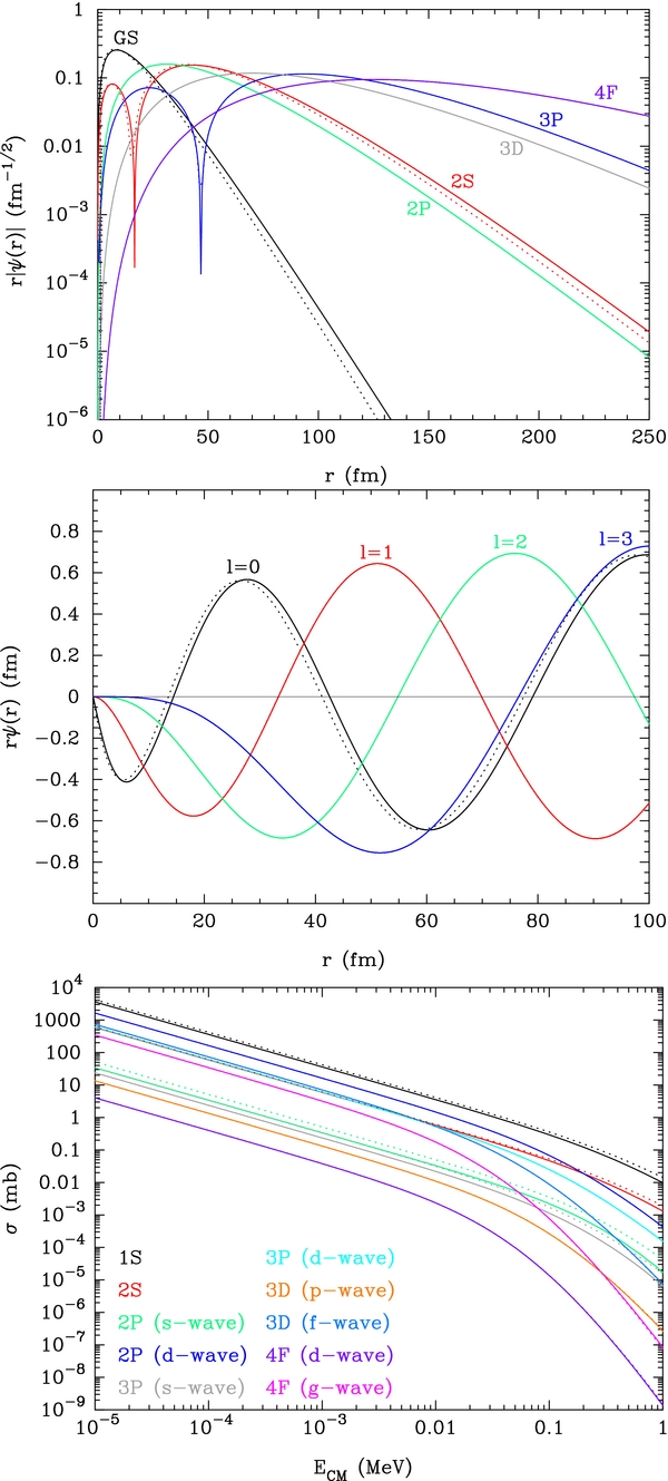
Figure 6. Bound-state wave functions (upper panel) and continuum wave functions at E = 3T/2 = 0.07 MeV (middle panel) for the 7Be+X− system as a function of radius r for the case of mX = 1 GeV. The bottom panel shows the recombination cross section as a function of CM energy E. In all panels, the solid lines correspond to calculated results while the dotted lines correspond to analytical formulae for hydrogen-like atomic states composed of two point-charges.
Download figure:
Standard image High-resolution imageThe bottom panel shows the recombination cross section as a function of the energy E. The solid lines correspond to the calculated results, while the dotted lines correspond to the analytical solution for the two point-charges (Equations (36), (37), and (41)). Partial cross sections for the following transitions are drawn: scattering p-wave → bound 1S state (1 black lines); p-wave → 2S (2 red); s-wave → 2P (3 green); d-wave → 2P (4 blue); s-wave → 3P (5 gray); d-wave → 3P (6 sky blue); p-wave → 3D (7 orange); f-wave → 3D (8 cyan); d-wave → 4F (9 violet); and g-wave → 4F (10 magenta). Dotted lines for point-charge nuclei correspond to transitions 1, 4, 8, 2 and 6 overlapping, 10, 3, 5, 7, and 9 in descending order of cross sections at E = 10−5 MeV. This order is true in all figures of recombination cross sections shown in this paper. The cross section of transition 2 is higher than that of transition 6 at high energies although they overlap at low energies. The order of solid lines at E = 10−5 MeV is the same as that of dotted lines. Since the mass mX is relatively small, the reduced mass is small and the spatial extent of the bound-state wave functions is large. The effect of a finite size charge distribution is only important for small r and is therefore small. Small differences in bound and scattering state wave functions lead to small changes in the cross sections through differences in the binding energies and wave function shapes. The largest differences in the cross sections are found for the two transitions starting from an initial s-wave, i.e., s-wave → 2P and s-wave → 3P. This is caused by differences in the scattering s-wave function.
Figure 7 shows bound-state wave functions (upper panel) and continuum wave functions (middle panel) at E = 0.07 MeV of the 7Be+X− system as a function of radius r for the case of mX = 10 GeV. Line types indicate the same quantities as in Figure 6. In the upper panel, the wave functions for the GS and 2S state in the finite charge distribution case (solid lines) deviate significantly from those for the point-charge case (dotted lines). Also, the wave functions for the 2P and 3P states deviate slightly. In the middle panel, the difference in the wave function for the l = 0 state is very large. A difference in the l = 1 state exists although it is not large. The bottom panel shows the recombination cross section as a function of energy E. Line types indicate the same quantities as in Figure 6. The order of solid lines at E = 10−5 MeV is 4, 1, 8, 6, 10, 2, 7, 9, 3, 5. Because of the larger mX value, the effect of a finite-size charge distribution is more important. Bound- and scattering-state wave functions and recombination cross sections are then significantly different from those for the point-charge case. Because of the large difference in the scattering s-wave function, the cross sections for transitions from an initial s-wave, i.e., s-wave → 2P and s-wave → 3P, are much smaller than those in the point-charge case. Partial cross sections for transitions from an initial p-wave to bound 1S, 2S and 3D states are also altered by the finite-size charge distribution. The cross sections for transitions to 1S and 2S states are also affected by differences in binding energies of the states between the finite- and point-charge cases.
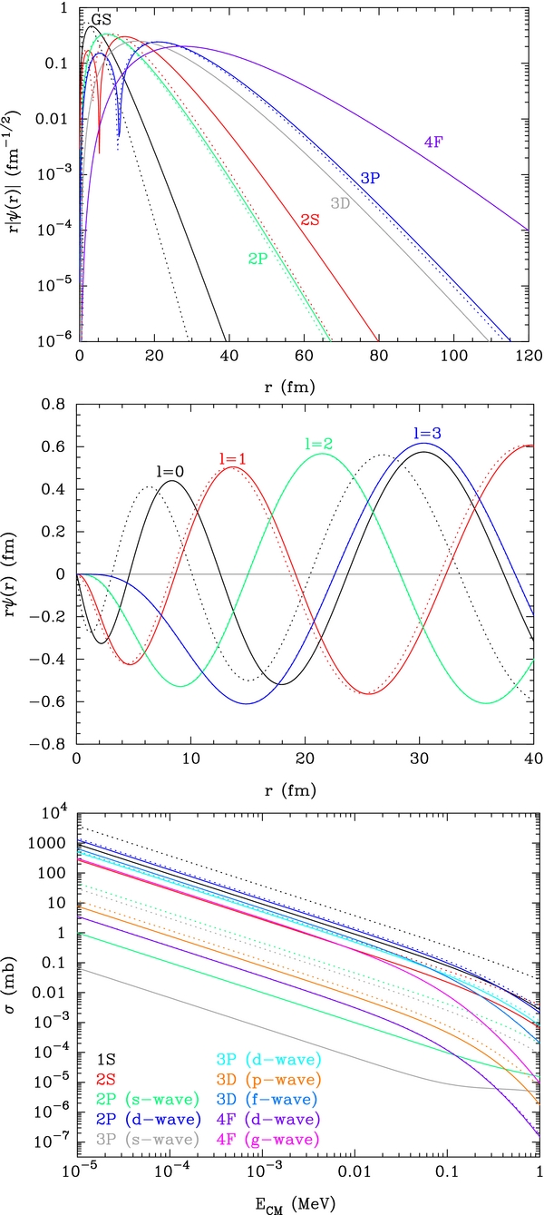
Figure 7. Same as Figure 6, but for mX = 10 GeV.
Download figure:
Standard image High-resolution imageFigure 8 shows bound-state wave functions (upper panel) and continuum wave functions (middle panel) at E = 0.07 MeV for the 7Be+X− system as a function of radius r for the case of mX = 100 GeV. Line types indicate the same quantities as in Figure 6. It is clear from a comparison of Figures 6–8 that deviations of the wave functions from those in the point-charge cases become larger as mX increases. We can see that deviations of wave functions for bound GS, 2S, 2P, and 3P states and scattering wave functions of l = 0 and l = 1 states are very large, and that a deviation exists for the l = 1 state, but it is not large. The bottom panel shows the recombination cross section as a function of the energy E. Line types indicate the same quantities as in Figure 6. The order of solid lines at E = 10−5 MeV is 4, 8, 6, 1, 10, 2, 9, 7, 3, 5. Differences in the solid and dotted lines are even larger than in the case of mX = 10 GeV (Figure 7).

Figure 8. Same as Figure 6 for the case of mX = 100 GeV.
Download figure:
Standard image High-resolution imageFigure 9 shows bound-state wave functions (upper panel) and continuum wave functions (middle panel) at E = 0.07 MeV as a function of radius r for the 7Be+X− system in the case of mX = 1000 GeV. Also shown is the recombination cross section as a function of the energy E (bottom panel). Thick solid and dotted lines indicate the same quantities as in Figure 6. The order of solid lines at E = 10−5 MeV is 4, 8, 6, 10, 1, 2, 9, 7, 3, 5. Since the reduced mass is similar to that in the case of mX = 100 GeV, this figure is rather similar to Figure 8. In order to check our calculations, we also calculate the wave functions and the cross sections for case of point-charge nuclei using the same code (a modified version of RADCAP) as used for the finite charge distribution case. Thin solid lines in the upper and middle panels show the calculated results which agree with analytical solutions (dotted lines) quite well.
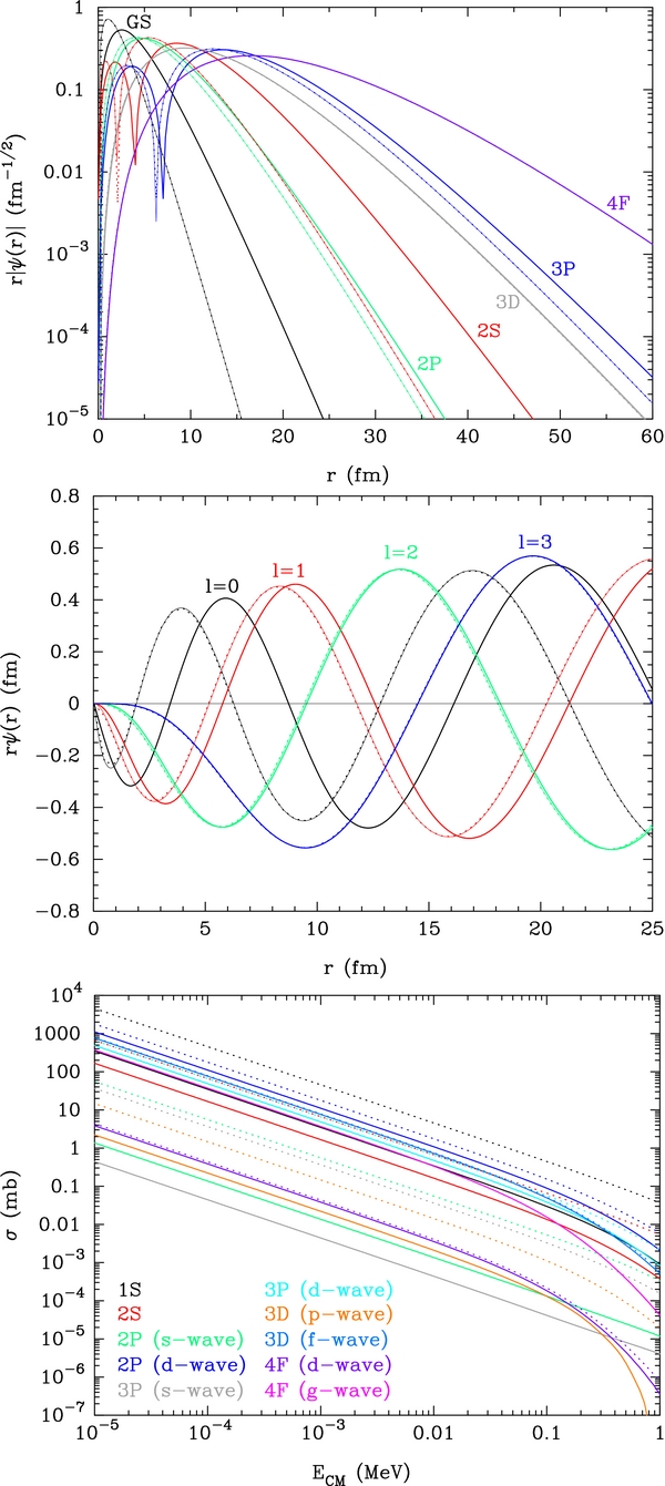
Figure 9. Same as Figure 6 for the case of mX = 1000 GeV. Thin solid lines in the upper and middle panels show results calculated under the assumption that 7Be has a point charge.
Download figure:
Standard image High-resolution imageWe found an important characteristic of the 7Be+X− recombination based upon our precise calculation including many transition channels. In the limit of a heavy X− particle, i.e., mX ≳ 100 GeV, the most important transition in the recombination is the d-wave → 2P. This fact does not hold in the case of the point-charge model. In that case, the transition p-wave → 1S is predominant (see the dotted lines in Figures 6–9). In the case of a finite size charge distribution, in addition to the main pathway of d-wave → 2P, cross sections for the transitions f-wave → 3D and d-wave → 3P are also larger than that for the GS formation. It is thus found that estimations of recombination cross sections taking into account only the GS as the final state may not be correct.
We note that our rate for mX = 1000 GeV is more than six times larger than the previous rate (Bird et al. 2008). We confirmed that the previous rate (Bird et al. 2008) is somewhat close to our rate when only taking into account the transition from the scattering p-wave to the bound 1S and 2S states. In Bird et al. (2008), it is described that the capture of 7Be directly to the GS of 7BeX has the largest cross section, closely followed by the capture to the 2S level. This is true for hydrogen-like ions composed of point-charged particles. However, we found that the most important transition is from the scattering d-wave to the bound 2P state. The previous rate (Bird et al. 2008) was adopted in most previous studies on BBN involving the X− particle, including studies by part of the present authors (Kusakabe et al. 2007, 2008, 2010). The nonresonant recombination rate is important for the 7Be destruction and also for constraining the parameter region for solving the Li problem. The significant improvement in the rate found in the present work therefore makes it possible to derive an improved constraint on the X− particle as shown in Section 8.
5.2. 7Li
5.2.1. Energy Levels
Table 9 shows binding energies for the 7LiX atomic states having main quantum numbers n from one to seven.
Table 9. Binding Energies of 7LiX Atomic States with Main Quantum Numbers n = 1–7 (keV)
| mX = 1 GeV | l = 0 | l = 1 | l = 2 | l = 3 | l = 4 | l = 5 | l = 6 |
|---|---|---|---|---|---|---|---|
| n = 1 | 198 | ||||||
| n = 2 | 50.7 | 52.0 | |||||
| n = 3 | 22.7 | 23.1 | 23.1 | ||||
| n = 4 | 12.8 | 13.0 | 13.0 | 13.0 | |||
| n = 5 | 8.23 | 8.31 | 8.31 | 8.31 | 8.31 | ||
| n = 6 | 5.73 | 5.77 | 5.77 | 5.77 | 5.77 | 5.77 | |
| n = 7 | 4.21 | 4.24 | 4.24 | 4.24 | 4.24 | 4.24 | 4.24 |
| mX = 10 GeV | l = 0 | l = 1 | l = 2 | l = 3 | l = 4 | l = 5 | l = 6 |
| n = 1 | 659 | ||||||
| n = 2 | 197 | 234 | |||||
| n = 3 | 92.9 | 104 | 105 | ||||
| n = 4 | 53.9 | 58.8 | 59.2 | 59.2 | |||
| n = 5 | 35.1 | 37.7 | 37.9 | 37.9 | 37.9 | ||
| n = 6 | 24.7 | 26.2 | 26.3 | 26.3 | 26.3 | 26.3 | |
| n = 7 | 18.3 | 19.2 | 19.3 | 19.3 | 19.3 | 19.3 | 19.3 |
| mX = 100 GeV | l = 0 | l = 1 | l = 2 | l = 3 | l = 4 | l = 5 | l = 6 |
| n = 1 | 847 | ||||||
| n = 2 | 277 | 354 | |||||
| n = 3 | 135 | 159 | 163 | ||||
| n = 4 | 79.5 | 89.9 | 91.8 | 91.9 | |||
| n = 5 | 52.4 | 57.7 | 58.8 | 58.8 | 58.8 | ||
| n = 6 | 37.1 | 40.2 | 40.8 | 40.8 | 40.8 | 40.8 | |
| n = 7 | 27.6 | 29.6 | 30.0 | 30.0 | 30.0 | 30.0 | 30.0 |
| mX = 1000 GeV | l = 0 | l = 1 | l = 2 | l = 3 | l = 4 | l = 5 | l = 6 |
| n = 1 | 872 | ||||||
| n = 2 | 289 | 372 | |||||
| n = 3 | 141 | 167 | 173 | ||||
| n = 4 | 83.6 | 94.8 | 97.1 | 97.2 | |||
| n = 5 | 55.1 | 61.0 | 62.2 | 62.2 | 62.2 | ||
| n = 6 | 39.0 | 42.5 | 43.2 | 43.2 | 43.2 | 43.2 | |
| n = 7 | 29.1 | 31.3 | 31.7 | 31.7 | 31.7 | 31.7 | 31.7 |
Download table as: ASCIITypeset image
5.2.2. 7Li(X−, γ)7LiX Resonant Rate
The resonant rates of the reaction 7Li(X−, γ)7LiX were calculated for mX = 1, 10, 100, and 1000 GeV in the WS40 model. The radius parameter for the WS40 model is R = 2.48 fm.
Table 10 shows calculated parameters of important transitions related to the reaction 7Li(X−, γ)7LiX for mX = 1, 100, and 1000 GeV. Similar to the recombination of 7Be+X−, the recombination can efficiently proceed via resonant reactions involving atomic states of  composed of the first nuclear excited state 7Li*[≡ 7Li*(0.478 MeV, 1/2−)]. Important resonances for
  satisfy EB ≲ 0.47761 MeV. We take into account atomic resonances with binding energies of 0.28 MeV ⩽EB ⩽ 0.48 MeV except for the atomic GS for the case of mX = 1 GeV. The transitions, matrix elements, radiative decay widths of the resonances, and resonance energies are listed in the second to fifth columns, respectively. For the case of mX = 1 GeV, there are no important resonances of atomic excited states because of the relatively small binding energies of 7LiX. The most important resonance in the recombination reaction is then the atomic GS of 7Li
 (1S), which can only decay into atomic states of the nuclear GS, i.e., 7Li
 and 7LiX. We take the measured rate for the radiative decay of 7Li* (Tilley et al. 2002) for the decay of 7Li
 (1S) into the GS 7LiX(1S).
Table 10. Calculated Parameters for 7Li(X−, γ)7LiX in the WS40 Model
| mX | Transition | τif | Γγ | Er |
|---|---|---|---|---|
| (GeV) | (fm) | (eV) | (MeV) | |
| 1 | 7Li (1S)→ 7LiX(1S) (1S)→ 7LiX(1S) |
⋅⋅⋅ | 0.00627a | 0.280 |
| 100 | 7Li (2P)→ 7Li (2P)→ 7Li (1S) (1S) |
3.91 | 1.26 | 0.124 |
| 1000 | 7Li (2P)→ 7Li (2P)→ 7Li (1S) (1S) |
3.81 | 1.34 | 0.105 |
Note.
aGiven by  with the lifetime 105 fs taken from that of the first excited 1/2− state of 7Li (Tilley et al. 2002).
Download table as: ASCIITypeset image
The resonant rates for the reaction 7Li(X−, γ)7LiX via Types 1 and 2 (only for mX = 1 GeV) transitions are derived to be
The rate for mX = 1 GeV corresponds to a pure nuclear transition from the resonance 7Li (1S) to the GS 7LiX(1S) (magnetic dipole transition Tilley et al. 2002). The rate for mX = 10 GeV is zero since there are no important resonances operating as a path for the recombination reaction. The rates for mX = 100 and 1000 GeV correspond to the atomic transition from the resonance 7Li
 (2P) to 7Li
 (1S).
(1S).
5.2.3. 7Li(X−, γ)7LiX Nonresonant Rate
The thermal nonresonant rate for the reaction 7Li(X−, γ)7LiX was derived as a function of temperature T by integrating the calculated cross section σ(E) over energy (Equation (10)). The derived rates are
Figure 10 shows bound-state wave functions (upper panel) and continuum wave functions (middle panel) at E = 0.07 MeV as a function of radius r for the 7Li+X− system with mX = 1 GeV. Also shown is the recombination cross section as a function of energy E (bottom panel). Line types indicate the same quantities as in Figure 6. The order of solid lines at E = 10−5 MeV is the same as that of dotted lines. In general, the trends of calculated results are similar to those of the 7Be+X− system (Figure 6). However, the Coulomb potential in the 7Li+X− system is smaller than that in the 7Be+X− system. Therefore, the spatial widths of wave functions in the former system are larger. The effect of the finite size of the charge distribution as shown by differences between the solid and dotted lines is then somewhat smaller in the 7Li+X− system than in the 7Be+X− system.

Figure 10. Same as Figure 6 for the 7Li+X− system with mX = 1 GeV.
Download figure:
Standard image High-resolution imageFigures 11–13 show bound-state wave functions (upper panel) and continuum wave functions (middle panel) at E = 0.07 MeV as a function of radius r for the 7Li+X− system in the case of mX = 10 GeV, 100 GeV, and 1000 GeV, respectively. Also shown is the recombination cross section as a function of the energy E (bottom panel). Line types indicate the same quantities as in Figure 6. The orders of solid lines at E = 10−5 MeV are 1, 4, 8, 6, 2, 10, 7, 9, 5, 3 in Figure 11, and 4, 1, 8, 6, 10, 2, 7, 9, 3, 5 in Figures 12 and 13, respectively. Similar to the case of the 7Be+X− system, larger mX values lead to larger differences in both the wave functions and the recombination cross sections between the finite-size charge and point-charge cases. We also find that this 7Li+X− system has the important characteristic that the transition d-wave → 2P is the most important for mX ≳ 100 GeV.
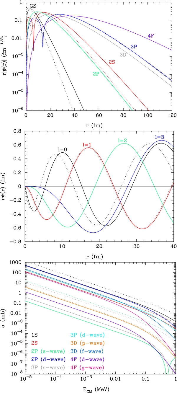
Figure 11. Same as Figure 6 for the 7Li+X− system with mX = 10 GeV.
Download figure:
Standard image High-resolution image
Figure 12. Same as Figure 6 for the 7Li+X− system with mX = 100 GeV.
Download figure:
Standard image High-resolution image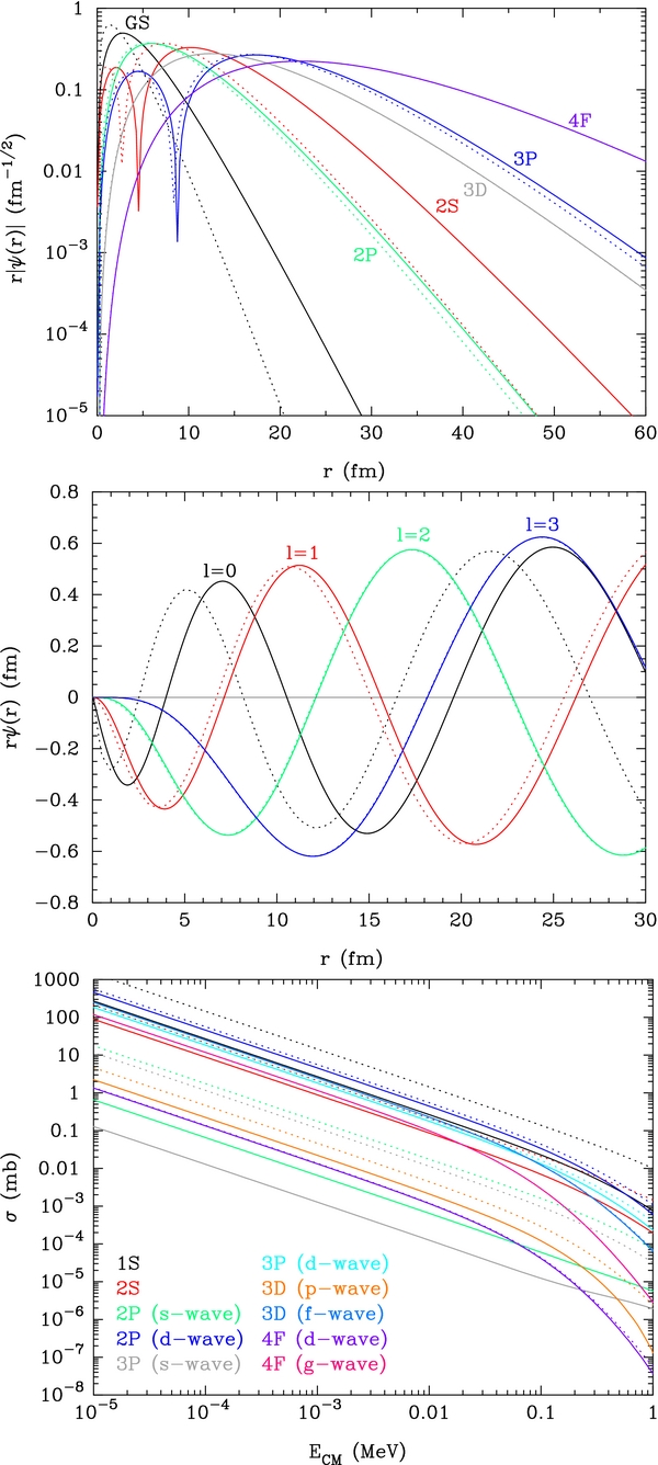
Figure 13. Same as Figure 6 for the 7Li+X− system with mX = 1000 GeV.
Download figure:
Standard image High-resolution image5.3. 9Be
5.3.1. Energy Levels
Table 11 shows the binding energies of 9BeX atomic states that have main quantum numbers n from one to seven.
Table 11. Binding Energies of 9BeX Atomic States with Main Quantum Numbers n = 1–7 (keV)
| mX = 1 GeV | l = 0 | l = 1 | l = 2 | l = 3 | l = 4 | l = 5 | l = 6 |
|---|---|---|---|---|---|---|---|
| n = 1 | 350 | ||||||
| n = 2 | 91.3 | 95.1 | |||||
| n = 3 | 41.1 | 42.3 | 42.3 | ||||
| n = 4 | 23.3 | 23.8 | 23.8 | 23.8 | |||
| n = 5 | 15.0 | 15.2 | 15.2 | 15.2 | 15.2 | ||
| n = 6 | 10.4 | 10.6 | 10.6 | 10.6 | 10.6 | 10.6 | |
| n = 7 | 7.68 | 7.77 | 7.77 | 7.77 | 7.77 | 7.77 | 7.77 |
| mX = 10 GeV | l = 0 | l = 1 | l = 2 | l = 3 | l = 4 | l = 5 | l = 6 |
| n = 1 | 1108 | ||||||
| n = 2 | 364 | 467 | |||||
| n = 3 | 178 | 210 | 216 | ||||
| n = 4 | 105 | 119 | 121 | 121 | |||
| n = 5 | 69.1 | 76.3 | 77.7 | 77.8 | 77.8 | ||
| n = 6 | 48.9 | 53.2 | 54.0 | 54.0 | 54.0 | 54.0 | |
| n = 7 | 36.4 | 39.1 | 39.7 | 39.7 | 39.7 | 39.7 | 39.7 |
| mX = 100 GeV | l = 0 | l = 1 | l = 2 | l = 3 | l = 4 | l = 5 | l = 6 |
| n = 1 | 1408 | ||||||
| n = 2 | 531 | 728 | |||||
| n = 3 | 272 | 335 | 364 | ||||
| n = 4 | 164 | 193 | 205 | 206 | |||
| n = 5 | 110 | 125 | 131 | 132 | 132 | ||
| n = 6 | 78.7 | 87.5 | 91.2 | 91.6 | 91.6 | 91.6 | |
| n = 7 | 59.0 | 64.7 | 67.0 | 67.3 | 67.3 | 67.3 | 67.3 |
| mX = 1000 GeV | l = 0 | l = 1 | l = 2 | l = 3 | l = 4 | l = 5 | l = 6 |
| n = 1 | 1448 | ||||||
| n = 2 | 558 | 768 | |||||
| n = 3 | 288 | 356 | 391 | ||||
| n = 4 | 175 | 205 | 220 | 222 | |||
| n = 5 | 117 | 133 | 141 | 142 | 142 | ||
| n = 6 | 83.9 | 93.4 | 97.8 | 98.5 | 98.5 | 98.5 | |
| n = 7 | 63.0 | 69.2 | 71.9 | 72.3 | 72.4 | 72.4 | 72.4 |
Download table as: ASCIITypeset image
5.3.2. 9Be(X−, γ)9BeX Nonresonant Rate
The nonresonant reaction rates for 9Be(X−, γ)9BeX were also calculated for mX = 1, 10, 100, and 1000 GeV in the WS40 model. The radius parameter for the WS40 model is R = 2.59 fm.
In the estimation of recombination rate for 9Be, the resonant reactions involving atomic states and nuclear excited states for 9Be* were neglected since even the first nuclear excited state has a large excitation energy of 1.684 MeV. We therefore only calculated the nonresonant rate.
The thermal nonresonant rate was derived as a function of temperature T by integrating the calculated cross section σ(E) over energy (Equation (10)). It is then
Figure 14 shows bound-state wave functions (upper panel) and continuum wave functions (middle panel) at E = 0.07 MeV as a function of radius r for the 9Be+X− system for the case of mX = 1 GeV. We also show recombination cross section as a function of the energy E (bottom panel). Line types indicate the same quantities as in Figure 6. The order of solid lines at E = 10−5 MeV is the same as that of the dotted lines. Trends of calculated results are similar to those of the 7Be+X− system (Figure 6).

Figure 14. Same as Figure 6 for the 9Be+X− system with mX = 1 GeV.
Download figure:
Standard image High-resolution imageFigures 15–17 show bound-state wave functions (upper panel) and continuum wave functions (middle panel) at E = 0.07 MeV as a function of radius r, and recombination cross sections as a function of the energy E (bottom panel) of the 9Be+X− system for the cases of mX = 10 GeV, 100 GeV, and 1000 GeV, respectively. Line types indicate the same quantities as in Figure 6. The orders of solid lines at E = 10−5 MeV are 4, 1, 8, 6, 10, 2, 7, 9, 3, 5 in Figure 15, and 4, 8, 6, 10, 1, 2, 9, 7, 3, 5 in Figures 16 and 17, respectively. Similar to the case of the 7Be+X− system, larger mX values lead to larger differences in wave functions and recombination cross sections between the finite-size charge and point-charge cases. We also find that the transition, d-wave → 2P, is most important for mX ≳ 100 GeV in this 9Be+X− system.

Figure 15. Same as Figure 6 for the 9Be+X− system with mX = 10 GeV.
Download figure:
Standard image High-resolution image
Figure 16. Same as Figure 6 for the 9Be+X− system with mX = 100 GeV.
Download figure:
Standard image High-resolution image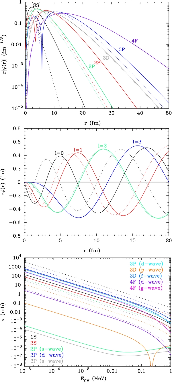
Figure 17. Same as Figure 6, but for the 9Be+X− system with mX = 1000 GeV.
Download figure:
Standard image High-resolution image5.4. 4He
5.4.1. Energy Levels
Table 12 shows the binding energies of 4HeX atomic states that have main quantum numbers n from one to seven.
Table 12. Binding Energies of 4HeX Atomic States with Main Quantum Numbers n = 1–7 (keV)
| mX = 1 GeV | l = 0 | l = 1 | l = 2 | l = 3 | l = 4 | l = 5 | l = 6 |
|---|---|---|---|---|---|---|---|
| n = 1 | 83.0 | ||||||
| n = 2 | 20.9 | 21.0 | |||||
| n = 3 | 9.29 | 9.33 | 9.33 | ||||
| n = 4 | 5.23 | 5.25 | 5.25 | 5.25 | |||
| n = 5 | 3.35 | 3.36 | 3.36 | 3.36 | 3.36 | ||
| n = 6 | 2.33 | 2.33 | 2.33 | 2.33 | 2.33 | 2.33 | |
| n = 7 | 1.71 | 1.71 | 1.71 | 1.71 | 1.71 | 1.71 | 1.71 |
| mX = 10 GeV | l = 0 | l = 1 | l = 2 | l = 3 | l = 4 | l = 5 | l = 6 |
| n = 1 | 263 | ||||||
| n = 2 | 69.0 | 72.3 | |||||
| n = 3 | 31.1 | 32.1 | 32.1 | ||||
| n = 4 | 17.7 | 18.1 | 18.1 | 18.1 | |||
| n = 5 | 11.4 | 11.6 | 11.6 | 11.6 | 11.6 | ||
| n = 6 | 7.92 | 8.03 | 8.03 | 8.03 | 8.03 | 8.03 | |
| n = 7 | 5.82 | 5.90 | 5.90 | 5.90 | 5.90 | 5.90 | 5.90 |
| mX = 100 GeV | l = 0 | l = 1 | l = 2 | l = 3 | l = 4 | l = 5 | l = 6 |
| n = 1 | 333 | ||||||
| n = 2 | 89.3 | 95.6 | |||||
| n = 3 | 40.6 | 42.5 | 42.5 | ||||
| n = 4 | 23.1 | 23.9 | 23.9 | 23.9 | |||
| n = 5 | 14.9 | 15.3 | 15.3 | 15.3 | 15.3 | ||
| n = 6 | 10.4 | 10.6 | 10.6 | 10.6 | 10.6 | 10.6 | |
| n = 7 | 7.66 | 7.81 | 7.81 | 7.81 | 7.81 | 7.81 | 7.81 |
| mX = 1000 GeV | l = 0 | l = 1 | l = 2 | l = 3 | l = 4 | l = 5 | l = 6 |
| n = 1 | 342 | ||||||
| n = 2 | 92.0 | 98.8 | |||||
| n = 3 | 41.9 | 43.9 | 43.9 | ||||
| n = 4 | 23.8 | 24.7 | 24.7 | 24.7 | |||
| n = 5 | 15.4 | 15.8 | 15.8 | 15.8 | 15.8 | ||
| n = 6 | 10.7 | 11.0 | 11.0 | 11.0 | 11.0 | 11.0 | |
| n = 7 | 7.91 | 8.07 | 8.07 | 8.07 | 8.07 | 8.07 | 8.07 |
Download table as: ASCIITypeset image
5.4.2. 4He(X−, γ)4HeX Nonresonant Rate
The nonresonant rates of the reaction 4He(X−, γ)4HeX were calculated for mX = 1, 10, 100, and 1000 GeV using the WS40 model. For this case, the radius parameter is R = 1.31 fm. Since all excited states of 4He* have excitation energies larger than 20 MeV, atomic states of nuclear excited states 4He are never important resonances in the recombination process. We then calculate only the nonresonant rate.
The thermal nonresonant rates were derived as a function of temperature T by integrating the calculated cross section σ(E) over energy (Equation (10)). The resultant rates are
Figure 18 shows bound-state wave functions (upper panel) and continuum wave functions (middle panel) at E = 0.07 MeV as a function of radius r for the 4He+X− system in the case of mX = 1 GeV. The recombination cross section is also given as a function of the energy E (bottom panel). Line types indicate the same quantities as in Figure 6. The order of solid lines at E = 10−5 MeV is the same as that of the dotted lines. Since the Coulomb potential in the 4He+X− system is small, the wave functions are more extended spatially. Therefore, the effect of the finite-size charge distribution is small as evidenced by the fact that the solid and dotted lines almost overlap in this figure.
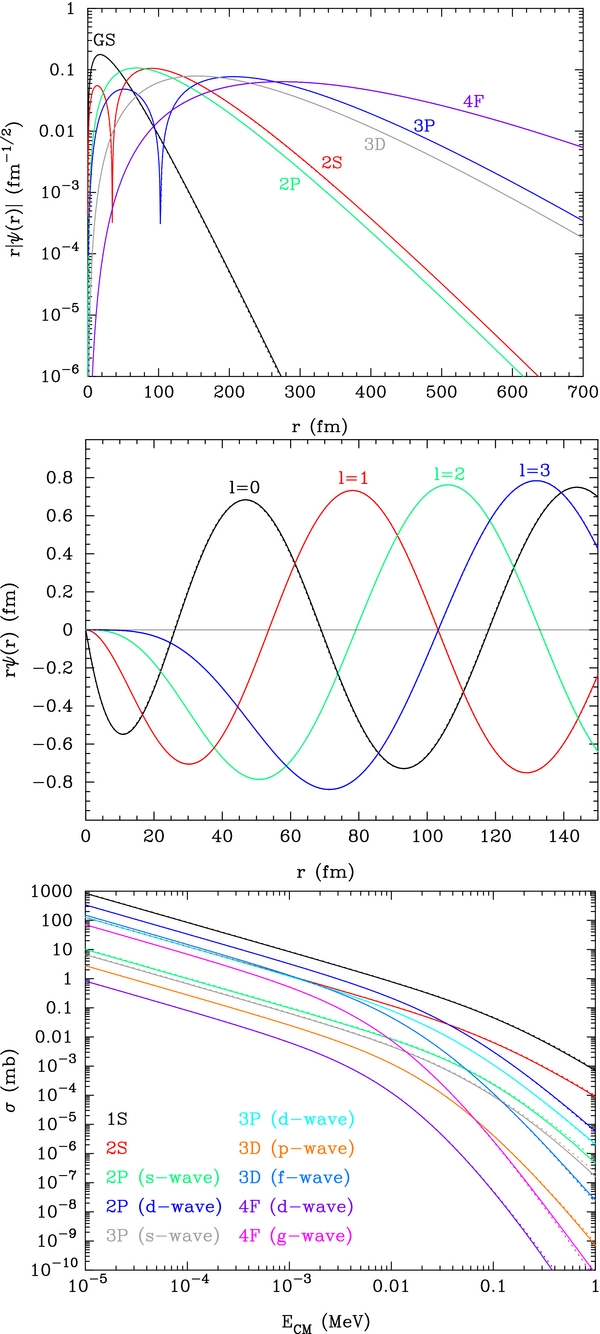
Figure 18. Same as Figure 6, but for the 4He+X− system with mX = 1 GeV.
Download figure:
Standard image High-resolution imageFigures 19–21 show bound-state wave functions (upper panel) and continuum wave functions (middle panel) at E = 0.07 MeV as a function of radius r for the 4He+X− system in the case of mX = 10 GeV, 100 GeV, and 1000 GeV, respectively. The recombination cross section is also shown as a function of the energy E (bottom panel). Line types indicate the same quantities as in Figure 6. In Figures 19–21, the orders of solid lines at E = 10−5 MeV are the same as that of the dotted lines. It is apparent that larger mX values lead to larger differences in the wave functions and recombination cross sections due to a finite-size versus a point-charge distribution. However, because of the small amplitude of the Coulomb potential, the effect of the finite-size nuclear charge does not significantly affect the wave functions and cross sections. As a result, even in the case of heavy X− particles (mX ≳ 100 GeV), the dominant transition contributing to the recombination is the p-wave → 1S, similarly to the case of the Coulomb potential for point charges.
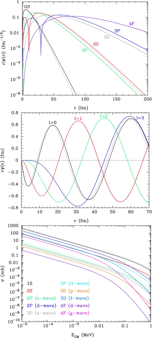
Figure 19. Same as Figure 6, but for the 4He+X− system with mX = 10 GeV.
Download figure:
Standard image High-resolution image
Figure 20. Same as Figure 6, but for the 4He+X− system with mX = 100 GeV.
Download figure:
Standard image High-resolution image
Figure 21. Same as Figure 6, but for the 4He+X− system with mX = 1000 GeV.
Download figure:
Standard image High-resolution image5.5. Other X-nuclei
As seen in the Sections 5.1–5.4, realistic wave functions and recombination cross sections for X-nuclei can be significantly different from those derived using two point-charged particles. Hence, the recombination rates based upon the Bohr atomic model that were utilized in the previous studies (e.g., Dimopoulos et al. 1990; de Rújula et al. 1990; Kohri & Takayama 2007; Kusakabe et al. 2007, 2008) should be considered uncertain by as much as one order of magnitude. Although precise recombination rates for minor nuclei are not yet derived, we assume that the Bohr atom formula (Bethe & Salpeter 1957) for the minor nuclei is sufficient. We adopt cross sections in the limit that the CM kinetic energy, E, is much smaller than the binding energy, EB. This is justified since the condition E = μv2/2 = 3T/2 ≪ EB with v the relative velocity of a nucleus A and X− always holds when the bound-state formation is more efficient than its destruction. The cross sections are thus given by
where e = 2.718 is the base of the natural logarithm. The thermal reaction rate is then given by
where Q9 = Q/MeV is the Q-value in units of MeV, and we defined a rate coefficient C1 = 1.37 × 10⁴(e1/e)2Q9/A5/2. The Q-value for the recombination is equal to the binding energy of the X-nucleus EB.
The thermal rate for reverse reaction is related to that for the forward reaction through the reciprocity theorem. Using the relation between the reverse rate 〈C + D〉 and the forward rate 〈A + B〉 (Fowler et al. 1967; Angulo et al. 1999), the reverse rate coefficient is defined for a non-radiative reaction A(B, C)D by
where gi = 2Ii + 1 accounts for the spin degrees of freedom with Ii the nuclear spin of species i. For a radiative reaction A(B, γ)C, on the other hand, the reverse rate coefficient is given by
where nγ = 2ζ(3)T3/π2 is the number density of photon with ζ(3) = 1.202 the Riemann zeta function of 3.
Table 13 shows approximate recombination rates for nuclei which are not treated in Section 5. The second and third columns correspond to the rate coefficients C1 and reverse rate coefficients Cr, respectively (Equations (58) and (60)), for the case of mX = 1 GeV. The C1 and Cr values for mX = 10, 100, and 1000 GeV are listed in the fourth to ninth columns.
Table 13. Approximate Recombination Rates
| Reaction | mX = 1 GeV | 10 GeV | 100 GeV | 1000 GeV | ||||
|---|---|---|---|---|---|---|---|---|
| C1 | Cr | C1 | Cr | C1 | Cr | C1 | Cr | |
| 1H(X−, γ)1HX | 1.05 × 10⁴ | 0.368 | 4.55 × 10³ | 0.863 | 4.04 × 10³ | 0.985 | 3.98 × 10³ | 0.985 |
| 2H(X−, γ)2HX | 6.77 × 10³ | 0.576 | 1.79 × 10³ | 2.160 | 1.42 × 10³ | 2.783 | 1.38 × 10³ | 2.783 |
| 3H(X−, γ)3HX | 5.61 × 10³ | 0.694 | 1.08 × 10³ | 3.543 | 7.74 × 10² | 5.106 | 7.45 × 10² | 5.106 |
| 3He(X−, γ)3HeX | 3.55 × 10⁴ | 0.694 | 1.30 × 10⁴ | 3.543 | 1.12 × 10⁴ | 5.106 | 1.10 × 10⁴ | 5.106 |
| 6Li(X−, γ)6LiX | 6.64 × 10⁴ | 0.857 | 1.76 × 10⁴ | 7.451 | 1.35 × 10⁴ | 14.38 | 1.31 × 10⁴ | 14.38 |
| 8Li(X−, γ)8LiX | 5.63 × 10⁴ | 0.909 | 1.13 × 10⁴ | 9.684 | 7.80 × 10³ | 22.08 | 7.46 × 10³ | 22.08 |
| 8B(X−, γ)8BX | 2.06 × 10⁵ | 0.909 | 5.53 × 10⁴ | 9.684 | 4.13 × 10⁴ | 22.08 | 3.98 × 10⁴ | 22.08 |
| 10B(X−, γ)10BX | 1.77 × 10⁵ | 0.942 | 3.83 × 10⁴ | 11.62 | 2.64 × 10⁴ | 30.77 | 2.52 × 10⁴ | 30.77 |
| 11B(X−, γ)11BX | 1.66 × 10⁵ | 0.954 | 3.26 × 10⁴ | 12.50 | 2.16 × 10⁴ | 35.45 | 2.05 × 10⁴ | 35.45 |
| 12B(X−, γ)12BX | 1.58 × 10⁵ | 0.965 | 2.86 × 10⁴ | 13.31 | 1.83 × 10⁴ | 40.34 | 1.73 × 10⁴ | 40.34 |
| 11C(X−, γ)11CX | 2.64 × 10⁵ | 0.954 | 5.83 × 10⁴ | 12.50 | 4.00 × 10⁴ | 35.45 | 3.80 × 10⁴ | 35.45 |
| 12C(X−, γ)12CX | 2.49 × 10⁵ | 0.965 | 5.01 × 10⁴ | 13.31 | 3.31 × 10⁴ | 40.34 | 3.13 × 10⁴ | 40.34 |
Download table as: ASCIITypeset image
6. 9Be PRODUCTION FROM 7Li
We suggest the possibility of a significant production of 9Be catalyzed by the negatively charged X− particle through the deuteron transfer reaction 7LiX(d, X−)9Be. This reaction rate depends on both resonant and nonresonant components. Since a realistic theoretical estimate of the rate for this reaction is not currently available, we adopt a simple ansatz that the astrophysical S factor for the reaction can be taken from the existing data for 7Li(d, nα)4He, i.e., S = 30 MeV b (Caughlan & Fowler 1988). We note that the cross section values for 7Li(d, nα)4He recommended by the Evaluated Nuclear Data File (ENDF/B-VII.1, 2011; Chadwick et al. 2011) correspond to S ∼ 10 MeV b for an energy range of 0.1 MeV ⩽E ⩽ 1 MeV.
Realistic theoretical estimates of the nonresonant cross section for 7LiX(d, X−)9Be would be difficult (M. Kamimura 2013, private communication). Since the structure of the 9Be nucleus is approximately described as α + α + n, there is no existing study on the probability that the 9Be nucleus is described as 7Li+d bound states. In addition, experiments on the low-energy nuclear scattering of 7Li+d are needed to construct the imaginary potential for 7Li+d elastic scattering in the quantum mechanical calculations. Hence, the cross section for 7LiX(d, X−)9Be assumed in this study is probably uncertain by as much as an order of magnitude, and could be much smaller.
7. β-DECAY AND NONRESONANT NUCLEAR REACTIONS
Mass excesses of X-nuclei and Q-values for possible reactions associated with the X− particle were calculated using the binding energies of X-nuclei derived in Section 3. The β-decay rates of X-nuclei (AX), ΓβX are estimated using experimental values for normal nuclei (A), Γβ, taking into account the momentum phase space factor related to the reaction Q-value. The adopted rates are then given by ΓβX = Γβ(QX/Q)5, where QX and Q are Q-values for the β-decay of AX and A, respectively. The decay rate Γβ is related to the half life T1/2, i.e., Γβ = ln 2/T1/2. An exception to this is the β-decay rate of 6BeX. In this case, the β-decay rate is estimated from that of 6He assuming an approximate isospin symmetry. Adopted data values are as follows: (1) Q = 3.508 MeV and Γβ = 0.859 s−1 for 6He(,  )6Li (Tilley et al. 2002), (2) Q = 16.005 MeV and Γβ = 0.825 s−1 for 8Li(,
  )8Be (Tilley et al. 2004), and (3) Q = 17.979 MeV and Γβ = 0.900 s−1 for 8B(, e+νe)8Be (Tilley et al. 2004).
Table 14 shows the adopted β-decay rates for X-nuclei. The second and third columns correspond to the Q-value and the decay rate ΓβX, respectively, for the case of mX = 1 GeV. The Q and ΓβX values for mX = 10, 100, and 1000 GeV are listed in the fourth to ninth columns.
Table 14. β-decay Rates
| Reaction | mX = 1 GeV | 10 GeV | 100 GeV | 1000 GeV | ||||
|---|---|---|---|---|---|---|---|---|
| QX (MeV) | ΓβX (s−1) | QX (MeV) | ΓβX (s−1) | QX (MeV) | ΓβX (s−1) | QX (MeV) | ΓβX (s−1) | |
| 6BeX(, e+νe)6LiX | 3.636 | 1.027 | 3.422 | 0.759 | 3.364 | 0.697 | 3.357 | 0.689 |
8LiX(,  )8BeX )8BeX |
16.407 | 0.934 | 15.915 | 0.802 | 15.704 | 0.750 | 15.676 | 0.744 |
| 8BX(, e+νe)8BeX | 17.296 | 0.742 | 17.095 | 0.699 | 17.054 | 0.691 | 17.049 | 0.690 |
Download table as: ASCIITypeset image
For nonresonant thermonuclear reaction rates between two charged nuclei, the astrophysical S-factors for X-nuclear reactions are taken to be as the same as those for the corresponding normal nuclear reactions (Caughlan & Fowler 1988; Smith et al. 1993). However, changes in the reduced mass and charge numbers are corrected exactly the same as in Kusakabe et al. (2008). For the reactions 6LiX(p, 3He)4HeX, 7BeX(p, γ)8BX, 4HeX(d, X−)6Li, 4HeX(t, X−)7Li, and 4HeX(3He, X−)7Be, the cross sections have been calculated in a quantum mechanical model (Hamaguchi et al. 2007; Kamimura et al. 2009). We therefore take those astrophysical S-factors from the published results, corrected for changes in the reduced mass. Since both forward and reverse reaction rates depend upon mX, they are different from the reaction rates estimated under the assumption of mX → ∞, which have been already published (Kusakabe et al. 2008).
For reactions between a neutron and X-nuclei and also those between nuclei and neutral X-nuclei, Coulomb repulsion does not exist. However, the reactions have already been found to be unimportant within the parameter region for which the predicted light element abundances are consistent with observational constraints (Kusakabe et al. 2010). We therefore utilize the same rates as assumed in Kusakabe et al. (2008) for the neutron-induced non-radiative reactions, and those published in Kamimura et al. (2009) for reactions of neutral X-nuclei.
Table 15 shows parameters of nuclear reaction rates for X-nuclei. The second and third columns correspond to the reverse rate coefficient Cr (Equations (59) and (60)) and the Q9-value, respectively, for the case of mX = 1 GeV. The Cr and Q9 values for mX = 10, 100, and 1000 GeV are listed in the fourth to ninth columns. Since the baryon density is low in the early universe, the rates for three-body reactions are small. Therefore, the reverse reactions of 6LiX(p, 3He α)X−, 7BeX(n, p7Li)X−, 7LiX(p, 2α)X−, and 1HX(7Li, 2α)X− are neglected in our calculation, and the reverse rate coefficients are not shown in this table.
Table 15. Reverse Reaction Coefficients and Q-values for Nuclear Reactions in the WS40 Model
| Reaction | mX = 1 GeV | 10 GeV | 100 GeV | 1000 GeV | ||||
|---|---|---|---|---|---|---|---|---|
| Cr | Q9 | Cr | Q9 | Cr | Q9 | Cr | Q9 | |
| 3HeX(d, p)4HeX | 6.108 | 213.050 | 7.641 | 213.536 | 8.376 | 213.822 | 8.478 | 213.862 |
| 3HeX(α, γ)7BeX | 1.415 | 21.464 | 2.690 | 27.768 | 3.742 | 30.115 | 3.925 | 30.421 |
| 4HeX(d, γ)6LiX | 1.695 | 18.390 | 2.305 | 21.182 | 2.716 | 22.238 | 2.782 | 22.375 |
| 4HeX(d, X−)6Li | 1.973 | 16.141 | 0.309 | 14.047 | 0.203 | 13.235 | 0.193 | 13.130 |
| 4HeX(t, γ)7LiX | 1.277 | 29.960 | 1.942 | 33.210 | 2.464 | 34.581 | 2.553 | 34.766 |
| 4HeX(t, X−)7Li | 1.438 | 27.662 | 0.225 | 25.567 | 0.148 | 24.756 | 0.141 | 24.651 |
| 4HeX(3He, γ)7BeX | 1.277 | 21.401 | 1.942 | 27.219 | 2.464 | 29.281 | 2.553 | 29.547 |
| 4HeX(3He, X−)7Be | 1.438 | 17.444 | 0.225 | 15.349 | 0.148 | 14.538 | 0.141 | 14.433 |
| 4HeX(α, γ)8BeX | 3.299 | 1.986 | 5.503 | 8.250 | 7.483 | 10.610 | 7.846 | 10.922 |
| 4HeX(6Li, γ)10BX | 1.927 | 56.985 | 3.723 | 66.752 | 5.745 | 70.332 | 6.163 | 70.811 |
| 6LiX(n, t)4HeX | 0.950 | 53.263 | 0.698 | 48.376 | 0.593 | 46.508 | 0.579 | 46.266 |
| 6LiX(p, γ)7BeX | 1.214 | 66.763 | 1.357 | 69.789 | 1.461 | 70.795 | 1.478 | 70.923 |
| 6LiX(p, 3He α)X− | ⋅⋅⋅ | 44.399 | ⋅⋅⋅ | 39.513 | ⋅⋅⋅ | 37.645 | ⋅⋅⋅ | 37.403 |
| 6LiX(α, γ)10BX | 1.727 | 55.699 | 2.453 | 62.675 | 3.212 | 65.199 | 3.364 | 65.539 |
| 7LiX(p, γ)8BeX | 6.622 | 201.967 | 7.267 | 204.981 | 7.788 | 205.969 | 7.879 | 206.096 |
| 7LiX(p, 2α)X− | ⋅⋅⋅ | 199.017 | ⋅⋅⋅ | 193.673 | ⋅⋅⋅ | 191.490 | ⋅⋅⋅ | 191.200 |
| 7LiX(α, γ)11BX | 4.317 | 104.484 | 5.818 | 111.338 | 7.497 | 113.795 | 7.850 | 114.130 |
| 8LiX(p, γ)9BeX | 2.111 | 197.719 | 2.285 | 200.809 | 2.438 | 201.835 | 2.467 | 201.968 |
| 6BeX(n, p)6LiX | 0.333 | 57.210 | 0.333 | 54.724 | 0.333 | 54.051 | 0.333 | 53.971 |
| 7BeX(n, p)7LiX | 1.000 | 17.422 | 1.000 | 14.854 | 1.000 | 14.164 | 1.000 | 14.083 |
| 7BeX(n, p7Li)X− | ⋅⋅⋅ | 15.124 | ⋅⋅⋅ | 7.212 | ⋅⋅⋅ | 4.338 | ⋅⋅⋅ | 3.968 |
| 7BeX(p, γ)8BX | 1.326 | 3.655 | 1.455 | 6.440 | 1.559 | 7.215 | 1.578 | 7.312 |
| 7BeX(d, p)8BeX | 14.24 | 193.572 | 15.63 | 194.019 | 16.75 | 194.317 | 16.95 | 194.363 |
| 7BeX(α, γ)11CX | 4.317 | 92.305 | 5.818 | 99.941 | 7.497 | 102.664 | 7.850 | 103.038 |
| 8BeX(p, γ)9BX | 2.111 | −0.081 | 2.285 | 2.688 | 2.438 | 3.446 | 2.467 | 3.541 |
| 9BeX(p, γ)10BX | 0.980 | 78.540 | 1.049 | 81.611 | 1.116 | 82.524 | 1.128 | 82.641 |
| 9BeX(p, 6Li)4HeX | 0.506 | 21.556 | 0.281 | 14.858 | 0.193 | 12.191 | 0.182 | 11.831 |
| 10BeX(p, γ)11BX | 0.433 | 132.395 | 0.459 | 135.205 | 0.487 | 135.932 | 0.492 | 136.023 |
| 9BX(p, γ)10CX | 6.846 | 49.053 | 7.326 | 53.070 | 7.789 | 54.451 | 7.879 | 54.637 |
| 10BX(p, γ)11CX | 3.030 | 103.370 | 3.215 | 107.055 | 3.406 | 108.260 | 3.445 | 108.422 |
| 11BX(p, γ)12CX | 7.002 | 187.715 | 7.375 | 191.414 | 7.791 | 192.632 | 7.879 | 192.797 |
| 1HX(α, p)4HeX | 2.090 | 0.815 | 5.686 | 2.793 | 7.679 | 3.582 | 7.967 | 3.684 |
| 1HX(7Li, 2α)X− | ⋅⋅⋅ | 201.168 | ⋅⋅⋅ | 201.050 | ⋅⋅⋅ | 201.028 | ⋅⋅⋅ | 201.026 |
| 1HX(7Be, X−)8B | 3.517 | 1.448 | 1.497 | 1.331 | 1.328 | 1.309 | 1.312 | 1.306 |
| 2HX(α, d)4HeX | 1.333 | 0.762 | 2.272 | 2.577 | 2.752 | 3.312 | 2.820 | 3.408 |
| 2HX(α, X−)6Li | 2.637 | 16.903 | 0.703 | 16.624 | 0.560 | 16.547 | 0.546 | 16.538 |
| 3HX(α, t)4HeX | 1.108 | 0.736 | 1.386 | 2.394 | 1.519 | 3.050 | 1.538 | 3.135 |
| 3HX(α, X−)7Li | 1.597 | 28.397 | 0.313 | 27.961 | 0.225 | 27.806 | 0.217 | 27.786 |
Download table as: ASCIITypeset image
Although the Q-value for the 8BeX(p, γ)9BX reaction is negative in the case of mX = 1 GeV, its rate is estimated by considering only the reduced mass factor. Since the |Q| value is very small, it can be regarded as effectively zero in the relevant temperature range.
8. BBN REACTION NETWORK
We utilized a modified (Kusakabe et al. 2008, 2010) version of the Kawano reaction network code (Kawano 1992; Smith et al. 1993) to calculate nucleosynthesis for four different X− particle masses, mX. The nuclear charge distribution was assumed to be given by the WS40 model. The free X− particle and bound X-nuclei are encoded as new species whose abundances are to be calculated. Reactions involving the X− particle are encoded as new reactions. The mass excesses of X-nuclei are input into the code. In this way, the energy generation through the recombination of normal nuclei and an X− particle, and the nuclear reactions of X-nuclei are precisely taken into account in the thermodynamics of the expanding universe (Kawano 1992).
Our BBN code includes many reactions associated with the X− particle. It then solves the non-equilibrium nuclear and chemical reaction network associated with the X− with improved reaction rates derived from quantum many-body calculations (Kamimura et al. 2009). The neutron lifetime was updated to be 878.5 ± 0.7stat ± 0.3sys s (Serebrov & Fomin 2010; Mathews et al. 2005) based upon improved measurements (Serebrov et al. 2005). Rates for reactions of normal nuclei with mass numbers A ⩽ 10 have been updated with the JINA REACLIB Database V1.0 (Cyburt et al. 2010). The baryon-to-photon ratio was taken from the WMAP determination (Spergel et al. 2003, 2007; Larson et al. 2011; Hinshaw et al. 2013) ΛCDM model (WMAP9 data only): i.e., η = (6.19 ± 0.14) × 10−10 (Hinshaw et al. 2013).
Reaction rates derived in this paper are included in the code. We note that the nonresonant radiative neutron capture reactions of X-nuclei considered in the previous study (Kusakabe et al. 2008) are switched off for the following reason. Rates for the reactions generally depend on mX. When mX is much larger than the nucleon mass, the radiative neutron capture reactions via electric multipole transitions are strongly hindered because of the very small effective charges (Kusakabe et al. 2009). In addition, independently of whether or not the mass of the mX is large, the nucleosynthesis triggered by the X− particle occurs rather late in the BBN epoch when the neutron abundance is already small. Thus, neglecting the reactions does not significantly change the time evolutions of the nuclear abundances.
Recombination rates for 7Be(X−, γ)7BeX, 7Li(X−, γ)7LiX, 9Be(X−, γ)9BeX, and 4He(X−, γ)4HeX were modified. 9BeX production through 8BeX, i.e., 4HeX(α, γ)8BeX(n, γ)9Be, depends significantly on the energy levels of 8BeX and 9BeX (Pospelov 2007a; Kamimura et al. 2009; Cyburt et al. 2012), and precise calculations with a quantum four-body model by another group is under way (Kamimura et al. 2010). In this paper, we neglect those reaction series and leave that discussion as a future work. The reaction 4HeX(α, γ)8BeX is thus not included, and the abundance of 8BeX is not shown in the figures below.
9. RESULTS
We show calculated results of BBN for four values of mX. First, we analyze the time evolution for abundances of normal and X-nuclei. Then, we update constraints on the parameters characterizing the X− particle.
The two free parameters in this BBN calculation are the ratio of number abundance of the X− particles to the total baryon density, YX = nX/nb, and the decay lifetime of the X− particle, τX. The lifetime is assumed to be much smaller than the age of the present universe, i.e., ≪14 Gyr (Hinshaw et al. 2013). The primordial X-particles from the early universe are thus by now long extinct. When the mX value is small, the annihilation cross section for the X− and its antiparticle X+ is expected to be large. Since a large cross section tends to a small freeze-out abundance of X−, it is naturally expected that the abundance YX would be very small for small mX. However, we also perform calculations for large values of YX even in the case of a small mX value taking into account the possibility that there may be a difference in number abundances of X− and X+. If the abundance of X− had been larger than X+, the freeze-out abundances could have been much larger than that for the case of equal abundances of X− and X+. In this case, however, charge neutrality still requires the condition of zero net global charge density during the BBN epoch.
As for the fate of X-nuclei, it is assumed that the total kinetic energy of products generated from the decay of the X− is large enough so that all X-nuclei can decay into normal nuclei plus the decay products of X−. The X particle is detached from X-nuclei with its rate given by the X− decay rate. The lifetime of X-nuclei is therefore given by the lifetime of the X− particle itself.
To identify the important reactions that affect the abundances of 6Li, 7Li, 7Be, and 9Be, we tried multiple calculations by switching off respective reactions. A detailed analysis of the nuclear flow is described below.
9.1. Abundance Constraints
Observational constraints on the deuterium abundance are taken from the mean value of 10 quasi-stellar object absorption line systems, and the abundance corresponding to the best measured damped Lyman alpha system of quasi-stellar object SDSS J1419+0829, i.e., log(D/H) = −4.58 ± 0.02 and log(D/H) = −4.596 ± 0.009, respectively (Pettini & Cooke 2012). Constraints on the primordial 3He abundance are taken from the mean value of Galactic H ii regions measured through the 8.665 GHz hyperfine transition of 3He+, i.e., 3He/H = (1.9 ± 0.6) × 10−5 (Bania et al. 2002). Constraints on the 4He abundance are taken from observational values of metal-poor extragalactic H ii regions, i.e., Yp = 0.2565 ± 0.0051 (Izotov & Thuan 2010) and Yp = 0.2561 ± 0.0108 (Aver et al. 2010). We take the observational constraint on the 7Li abundance from the central value of log(7Li/H) =−12 + (2.199 ± 0.086) derived in the 3D NLTE model of Sbordone et al. (2010). On the other hand, the constraint on the 6Li abundance is chosen more conservatively. We adopted the least stringent 2σ (95% C.L.) upper limit for all stars reported in Lind et al. (2013), i.e., 6Li/H = (0.9 ± 4.3) × 10−12 for the G64-12 (NLTE model with five free parameters).
9.2. mX = 1 GeV
9.2.1. Nucleosynthesis
Figure 22 shows the calculated abundances of normal nuclei (panel (a)) and X nuclei (panel (b)) as a function of T9 for mX = 1 GeV. Curves for 1H and 4He correspond to the mass fractions, Xp (1H) and Yp (4He) in total baryonic matter, while the other curves correspond to number abundances with respect to that of hydrogen. The dotted lines show the result of the SBBN model. The abundance and the lifetime of the X− particle are assumed to be YX = 0.05 and τX = ∞, respectively, for this example.
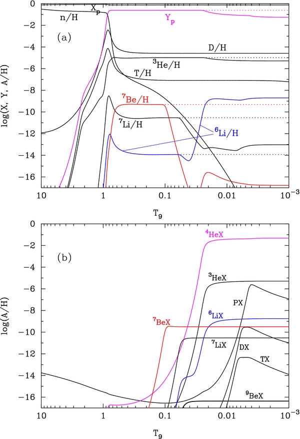
Figure 22. Calculated abundances of normal nuclei (a) and X-nuclei (b) as a function of T9 for mX = 1 GeV. Xp and Yp are the mass fractions of 1H and 4He, in total baryonic matter, while the other curves correspond to number abundances with respect to that of hydrogen. The abundance and lifetime of the X− particle are taken to be YX = nX/nb = 0.05 and τX = ∞, respectively. The dotted lines show the results of the SBBN model.
Download figure:
Standard image High-resolution imageEarly in the BBN epoch (T9 ≳ 1), pX is the only X-nuclide with an abundance larger than AX/H >10−17. Its abundance is the equilibrium value determined by the balance between the recombination of p and X− and the photoionization of pX. When the temperature decreases to T9 ≲ 1, 4He is produced as in SBBN (panel (a)). Simultaneously, the abundance of 4HeX increases through the recombination of 4He and X− (panel (b)). As the temperature decreases further, the recombination of nuclei with X− gradually proceeds in order of decreasing binding energies of AX, similar to the recombination of nuclei with electrons.
7Be first recombines with X− via the 7Be(X−, γ)7BeX reaction at T9 ≲ 0.1. The produced 7BeX nuclei are then slightly destroyed via the 7BeX(p, γ)8BX reaction. In the late epoch, the 7Be abundance increases through the reaction 4HeX(3He, X−)7Be at T9 ∼ 0.03–0.02.
The 6Li abundance decreases through the recombination reaction 6Li(X−, γ)6LiX operating at T9 ≲ 0.05. However, soon after the start of recombination, it is produced through the reaction 4HeX(d, X−)6Li at T9 ∼ 0.03–0.02. After this production, the 6LiX abundance also increases through recombination. In the late epoch, the 6Li abundance increases through the reaction 2HX(α, X−)6Li at T9 ∼ 4 × 10⁻³.
At T9 ≲ 0.05, the 7Li abundance decreases through the recombination reaction 7Li(X−, γ)7LiX. A small amount of 7Li is later produced through the reactions 4HeX(t, X−)7Li (T9 ∼ 0.02–0.01), and 3HX(α, X−)7Li [T9 ∼ (6–5) × 10−3].
9Be is predominantly produced through the reaction 7LiX(d, X−)9Be at T9 ∼ 0.06–0.05. At T9 ≲ 0.05, the recombination 9Be(X−, γ)9BeX enhances the abundance of 9BeX. The abundance of 9Be is small and not seen in this figure since it is converted to 9BeX via the recombination. We note that the proton capture reaction 9BeX(p, 6Li)4HeX does not work efficiently at this temperature of 9BeX production.
The recombination of 7Be with an X− particle and the subsequent radiative proton capture of 7BeX occurs at T9 ∼ 0.1 although the effect of the latter reaction cannot be seen well in this figure. In this case, the abundances of 7Be and 7BeX only change through the recombination at T9 ∼ 0.1. The abundance ratio of 7Be to 7BeX is then simply described with chemical equilibrium (Rybicki & Lightman 1979) as
where the spin factor of X− is gX = 1 and only the GS of 7BeX is considered so that  .
.
The baryon number density determined from the CMB WMAP measurement is
where ρb and ρc are the baryon density and the present critical density, respectively. Ωb = 0.0463 ± 0.0024 is the baryon density parameter, z is the redshift of the universe, which is related to temperature as (1 + z) = T/T0 where T0 = 2.7255 K is the present radiation temperature of the universe (Fixsen 2009), and h = H0/(100 km s−1 Mpc−1) =0.700 ± 0.022 is the reduced Hubble constant with Hubble constant H0. The cosmological parameters have been taken from values determined from the WMAP (Spergel et al. 2003, 2007; Larson et al. 2011; Hinshaw et al. 2013) (ΛCDM model; WMAP9 data only).
We define the recombination temperature Trec(A) at which abundances of the ionized nuclei A and the bound state AX are equal. The Trec(A) value is determined as a function of the abundance of X−, YX, using Equations (61) and (62). For example, the recombination temperature of 7Be for the case of mX = 1 GeV and YX = 0.05 is Trec(7Be) = 8.49 keV (corresponding to T9 = 0.0985). Since the recombination proceeds at temperatures lower than in the case of larger mX, the number density of protons at recombination is smaller. As a result, the rate for 7BeX to experience radiative proton capture in the temperature range of T9 ≲ 0.1 is small. The reduction of the 7BeX abundance through the proton capture is therefore less efficient than in the cases with mX = 100 GeV and 1000 GeV. However, it is still much more efficient than the case with mX = 10 GeV because of the smaller resonant energy in the resonant reaction 7BeX(p, γ)8BX (see Section 4).
9.2.2. Constraints on the X− Particle
Figure 23 shows contours of calculated final lithium abundances for the case of mX = 1 GeV. These are normalized to the values observed in MPSs, i.e., d(6Li) = 6LiCal/6LiObs (blue lines) and d(7Li) = 7LiCal/7LiObs (red lines). The final 7Li abundance is a sum of the abundances of 7Li and 7Be produced in BBN. This is because 7Be is converted to 7Li via the electron capture at a later epoch. The dashed lines around the line of d(7Li) = 1 correspond to the 2σ uncertainty in the observational constraint. The gray region located to the right of the contours for d(6Li) = 10 and/or the 2σ lower limit, d(7Li) = 0.67, are excluded by the overproduction of 6Li and underproduction of 7Li, respectively. The orange region is the interesting parameter region in which a significant 7Li reduction occurs without inducing an overproduction of 6Li. Dotted lines are contours of the calculated abundance ratio of 9Be/H assuming a rate for the reaction 7LiX(d, X−)9Be as described above in Section 6.

Figure 23. Contours of constant lithium abundances relative to the observed values in MPSs, i.e., d(6Li) = 6LiCal/6LiObs (blue lines) and d(7Li) = 7LiCal/7LiObs (red lines) for the case of mX = 1 GeV. The adopted observational constraint on the 7Li abundance is the central value of log(7Li/H) =−12 + (2.199 ± 0.086) derived in the 3D NLTE model of Sbordone et al. (2010). The 6Li constraint is taken from the 2σ upper limit for the G64-12 (NLTE model with five parameters; Lind et al. 2013) of 6Li/H = (0.9 ± 4.3) × 10−12. Dashed lines around the line of d(7Li) = 1 correspond to the 2σ uncertainty in the observational constraint. The gray region located to the right from the contours of d(6Li) = 10 or the 2σ lower limit, d(7Li) = 0.67, is excluded by the overproduction of 6Li and underproduction of 7Li, respectively. The orange region is the interesting parameter region in which a significant reduction in 7Li is realized without an overproduction of 6Li. Dotted lines are contours of the abundance ratio of 9Be/H predicted when the unknown rate for the reaction 7LiX(d, X−)9Be is adopted as described in the text.
Download figure:
Standard image High-resolution imageIf the X− lifetime is long enough, larger X− abundances lead to more production of 6Li. This is because the production rate of 6Li through the reaction 4HeX(d, X−)6Li is proportional to the abundance of 4HeX which is proportional to the X− abundance as long as nX ⩽ nα. On the other hand, for large YX values the amount of 7Be destruction is not proportional to the X− abundance. The reason is that the amount of 7Be destruction roughly depends upon the recombination temperature and the conversion rate of 7BeX through the reaction 7BeX(p, γ)8BX. However, the recombination temperature is almost independent of YX. Therefore, the conversion rate is independent of YX although it is dependent on np. The destruction is therefore not efficient even if the YX values were very high.
The excluded gray region corresponds to YX ≳ 10−3 in the limit of a long X−-particle lifetime τX ≳ 108 s. This region is determined from the overproduction of 6Li. The orange region corresponding to a solution to the 7Li problem is located at YX ≳ 0.1 and τX ∼ 5 × 10³–105 s. Within this region, the primordial 9Be abundance is predicted to be 9Be/H ≲ 3 × 10⁻¹⁶. This is much larger than the SBBN value of 9.60 × 10⁻¹⁹ (Coc et al. 2012). Since the abundances of D, 3He, and 4He are not significantly altered, the adopted constraints on their primordial abundances are satisfied in this region.
Figure 24 shows the same contours for calculated abundances of 6, 7Li and 9Be as in Figure 23. In this case, the instantaneous charged-current decay of 7BeX → 7Li+X0 (Jittoh et al. 2007, 2008, 2010; Bird et al. 2008) is also taken into account. In this case, the X− particle interacts not only via its charge but also a weak interaction (Jittoh et al. 2007, 2008, 2010). 7BeX can then be converted to 7Li plus a neutral particle X0. Other X-nuclei may also decay depending upon the mass of the X0. The prohibition of 6Li overproduction, however, limits the length of the lifetime of the X− as seen in Figure 23. Effects of the weak decay catalyzed by the X− then appear through the conversion of X-nuclei produced just before the epoch of 6Li production.

Figure 24. Same as in Figure 23, but the charged-current decay of 7BeX → 7Li+X0 is also included.
Download figure:
Standard image High-resolution imageAbove the recombination temperature for 4HeX at which 6Li production also proceeds, 6LiX, 7LiX, and 7BeX can all be produced with large fractions of bound states (see Figure 22). Among these three X-nuclei, 7BeX is the most abundant and its abundance evolution affects the parameter region for a solution to the Li problem. Therefore, for simplicity, we only consider the decay of 7BeX here.
The contours for the 6Li abundance are similar to those in Figure 23. On the other hand, the 7Li abundance is much different from that in Figure 23 because of the different processes for 7Be destruction. Including the charged-current decay of 7BeX, the destruction rate of 7Be in this model is the same as the recombination rate of 7Be itself. In the model without the decay, the destruction rate requires that 7BeX nuclei produced via the recombination then experience a proton capture reaction without being re-ionized to a 7Be+X− free state. The different processes of 7BeX destruction therefore cause a difference in the efficiency for the final 7Li reduction. In this model with the decay, the amount of 7Be destruction roughly scales as YX unlike the model without the decay.
The excluded region is wider than in Figure 23. This region is determined from the 7Li underproduction. This region also involves lower values of τX than in Figure 23. The solution to the 7Li problem is at YX ≳ 8 × 10⁻⁴ and τX ≳ 102 s (orange region). In this region, the 9Be abundance is calculated to be 9Be/H ≲3 × 10⁻¹⁷.
9.3. mX = 10 GeV
9.3.1. Nucleosynthesis
Figure 25 shows the same abundances as a function of T9 as in Figure 22, but for the case of mX = 10 GeV and without the decay of 7BeX.
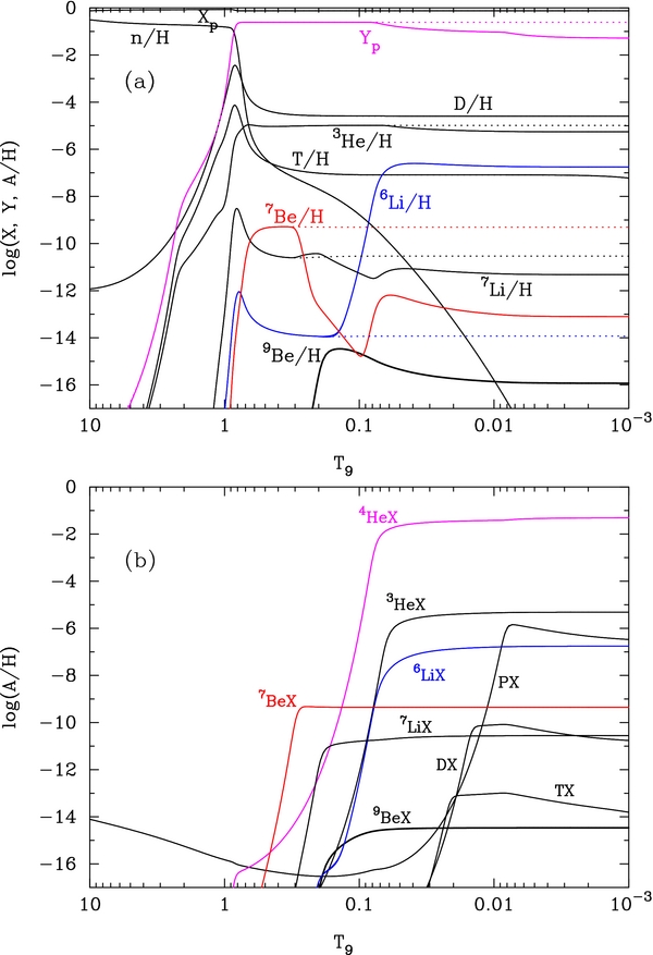
Figure 25. Same as in Figure 22, but for the case of mX = 10 GeV.
Download figure:
Standard image High-resolution imageThe 7Be nuclide recombines with X− at Trec(7Be) = 25.1 keV (T9 = 0.291). Although this temperature is higher than in the case of mX = 1 GeV, the resonant peak in the 7BeX(p, γ)8BX reaction is higher. The efficiency for 7BeX destruction is then smaller than that for mX = 1 GeV. During a late epoch, the 7Be abundance increases mainly through the reaction 4HeX(3He, X−)7Be at T9 ≲ 0.1. In the same epoch, the 7Be abundance increases also through the reaction 6Li(p, γ)7Be. However, in this case the production rate is much smaller than that via 4HeX(3He, X−)7Be. It is thus found that 7Be is produced by the 6Li(p, γ)7Be reaction if the abundance of 6Li during BBN is much larger than in SBBN as realized in this model by including the X− particle.
6Li is produced through the reaction 4HeX(d, X−)6Li at T9 ∼ 0.06. 6LiX is then produced through the recombination 6Li(X−, γ)6LiX.
At first the 7Li abundance increases through the two reaction pathways of 7BeX(n, p7Li)X− and 7BeX(n, p)7LiX(γ, X−)7Li at T9 ∼ 0.3–0.2. This is seen as a bump in the abundance curve. The existence of this bump depends upon the reaction rates of 7BeX(n, p7Li)X− and 7BeX(n, p)7LiX, which are assumed to be the same as that of 7Be(n, p)7Li in this paper. This possible bump appears during the epoch when the recombination of 7Be has started but that of 7Li has not. Then, the 7Li abundance decreases through the recombination reaction 7Li(X−, γ)7LiX at T9 ∼ 0.2–0.1. The proton capture reaction 7LiX(p, 2α)X− also partly destroys the 7LiX nuclei produced via the recombination. Finally, 7Li is produced through the reaction 4HeX(t, X−)7Li at T9 ∼ 0.07–0.06.
9Be is produced through the reaction 7LiX(d, X−)9Be at T9 ∼ 0.2–0.1. The recombination of 9Be increases the abundance of 9BeX at T9 ∼ 0.2–0.1. When the proton-capture reaction 9BeX(p, 6Li)4HeX is operative at T9 ≳ 0.07, it decreases the abundance of 9BeX.
9.3.2. Constraints on the X− Particle
Figure 26 shows the same contours for calculated abundances of 6, 7Li and 9Be as in Figure 23 without the decay of 7BeX, but for mX = 10 GeV. The excluded gray region is larger than that in Figure 23 because of the enhanced production rate of 6Li. In addition, there is no parameter region for the solution to the 7Li problem because of the smaller destruction rate for 7Be.
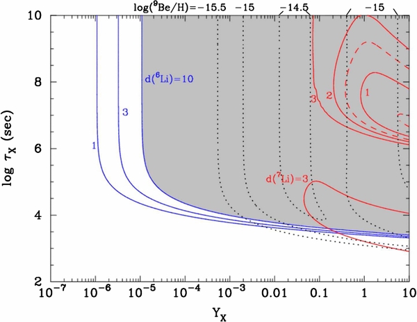
Figure 26. Same as in Figure 23, but for the case of mX = 10 GeV. Note that there is no interesting parameter region in which a 7Li reduction occurs without an overproduction of 6Li.
Download figure:
Standard image High-resolution imageFigure 27 shows the same contours for calculated abundances of 6, 7Li and 9Be as in Figure 23, but for mX = 10 GeV and with the decay of 7BeX. The contours for the 6Li abundance are similar to those in Figure 26. The 7Li abundance is different from that in Figure 25 for the same reason described above for Figure 24. The excluded region is determined from the combination of 7Li underproduction and 6Li overproduction. It is wider than in Figure 26. The region for the 7Li problem is at YX ≳ 10−3 and τX ∼ 102–104 s. The 9Be abundance in this region is 9Be/H ≲ 10−15.
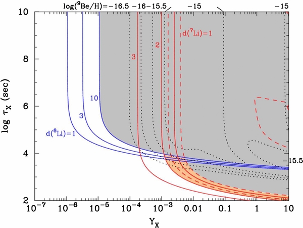
Figure 27. Same as in Figure 23, but for the case of mX = 10 GeV when the charged-current decay of 7BeX → 7Li+X0 is included.
Download figure:
Standard image High-resolution image9.4. mX = 100 GeV
9.4.1. Nucleosynthesis
Figure 28 shows the same abundances as a function of T9 as in Figure 22 without the decay of 7BeX, but for the case of mX = 100 GeV.

Figure 28. Same as in Figure 22, but for the case of mX = 100 GeV.
Download figure:
Standard image High-resolution imageThe 7Be nuclide recombines with X− at Trec(7Be) = 30.9 keV (T9 = 0.359). The efficiency of 7BeX destruction through the reaction 7BeX(p, γ)8BX at T9 = 0.3–0.2 is larger than in the cases with mX = 1 GeV and 10 GeV as seen in this figure. This high efficiency is because of the higher recombination temperature and the relatively smaller peak of the resonant reaction 7BeX(p, γ)8BX. During the later epoch, the 7Be abundance increases mainly through the reaction 4HeX(3He, X−)7Be and somewhat less through the reaction 6Li(p, γ)7Be.
6Li is produced through the reaction 4HeX(d, X−)6Li at T9 ∼ 0.1. The abundance of 6LiX increases through the recombination reaction 6Li(X−, γ)6LiX. Some of the 6LiX nuclei are then destroyed through proton capture via the 6LiX(p, 3Heα)X− reaction in the temperature range of T9 ≳ 0.05.
In the interval of recombination temperatures for 7Be and 7Li, i.e., T9 ∼ 0.3–0.2, the 7Li abundance at first increases through the neutron-induced reactions on 7BeX as in the case of mX = 10 GeV. Then, the 7Li abundance decreases through recombination with X− at T9 ≲ 0.2. At T9 ≳ 0.05, the proton capture reaction 7LiX(p, 2α)X− partly destroys 7LiX nuclei produced via the recombination. Finally, 7Li is produced through the reaction 4HeX(t, X−)7Li at T9 ≲ 0.1.
9Be is produced through the reaction 7LiX(d, X−)9Be at T9 ∼ 0.3–0.1. The recombination 9Be(X−, γ)9BeX reaction enhances the abundance of 9BeXat T9 ∼ 0.2–0.1. The proton capture reaction 9BeX(p, 6Li)4HeX then decreases the abundance of 9BeX at T9 ≳ 0.1.
9.4.2. Constraints on the X− Particle
Figure 29 shows the same contours for calculated abundances of 6, 7Li and 9Be as in Figure 23 without the decay of 7BeX, but for mX = 100 GeV. The excluded gray region is even larger than that for mX = 10 GeV because of the enhanced production rate of 6Li. The parameter region for the solution to the 7Li problem is at YX ≳ 0.07 and τX ∼ (0.6–3) × 103 s. The 9Be abundance in this region is 9Be/H ≲ 3 × 10⁻¹⁶.
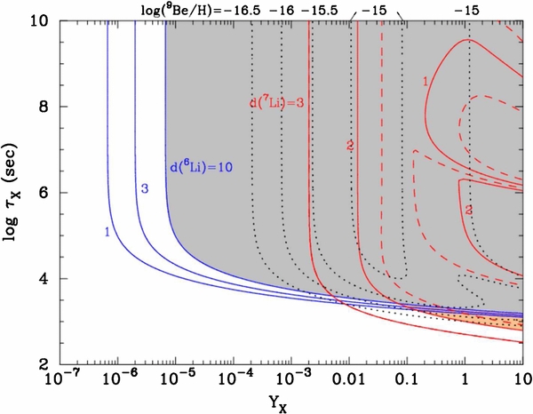
Figure 29. Same as in Figure 23, but for the case of mX = 100 GeV.
Download figure:
Standard image High-resolution imageFigure 30 shows the same contours for calculated abundances of 6, 7Li and 9Be as in Figure 23, but for mX = 100 GeV and with the decay of 7BeX. The excluded region is determined from the combination of the 7Li underproduction and the 6Li overproduction. The region for the 7Li problem is at YX ≳ 6 × 10⁻³ and τX ∼ 102–4 × 10³ s. In this region, the 9Be abundance is 9Be/H ≲ 3 × 10⁻¹⁶.
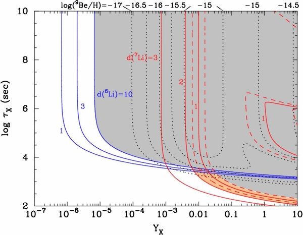
Figure 30. Same as in Figure 23, but for the case of mX = 100 GeV and the charged-current decay of 7BeX → 7Li+X0 is included.
Download figure:
Standard image High-resolution image9.5. mX = 1000 GeV
9.5.1. Nucleosynthesis
Figure 31 shows the same abundances as a function of T9 as in Figure 22 without the decay of 7BeX, but for the case of mX = 1000 GeV. This result is very similar to that for mX = 100 GeV except for the abundance of 7BeX.
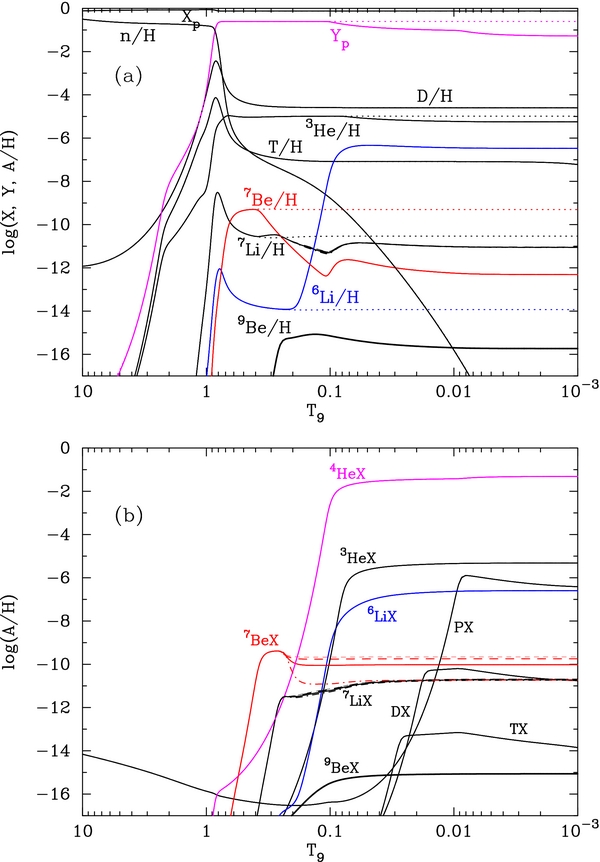
Figure 31. Same as in Figure 22, but for the case of mX = 1000 GeV.
Download figure:
Standard image High-resolution imageThe recombination temperature of 7Be is the same as in the case of mX = 100 GeV, i.e., Trec(7Be) = 30.9 keV (T9 = 0.359). The efficiency of 7BeX destruction through the reaction 7BeX(p, γ)8BX is slightly larger than that for mX = 100 GeV mainly because of the lower resonance energy of the reaction 7BeX(p, γ)8BX.
BBN calculations for mX = 1000 GeV are performed for four cases of reaction rates for 7BeX(p, γ)8BX and 8BeX(p, γ)9BX. Three cases correspond to Gaussian (thick dashed lines), WS40 (solid lines), and square well (dot–dashed lines) models for nuclear charge distributions studied in this paper (Section 4), while one case (thin dashed lines) corresponds to the previous calculation (Kusakabe et al. 2008) in which the adopted reaction rate for 7BeX(p, γ)8BX was derived from a quantum many-body model (Kamimura et al. 2009). It is found that amounts of 7BeX destruction vary significantly when the nuclear charge distributions are changed. The result for our Gaussian charge distribution model (thick dashed line) is close to that for the quantum many-body model (thin dashed line slightly above the thick dashed line) in which the charge distribution of the cluster components has also been assumed to be Gaussian. The differences in the curves for 7BeX thus indicate the effect of uncertainties in the charge density inferred from measurements of rms radii.
9.5.2. Constraints on the X− Particle
Figure 32 shows the same contours for calculated abundances of 6, 7Li and 9Be as in Figure 23 without the decay of 7BeX, but for mX = 1000 GeV. The parameter region for the solution to the 7Li problem is at YX ≳ 0.04 and τX ∼ (0.6–3) × 103 s. The 9Be abundance in this region is 9Be/H ≲ 3 × 10⁻¹⁶.

Figure 32. Same as in Figure 23, but for the case of mX = 1000 GeV.
Download figure:
Standard image High-resolution imageFigure 33 shows the same contours for calculated abundances of 6, 7Li and 9Be as in Figure 23, but for mX = 1000 GeV and with the decay of 7BeX also included. The region for the solution of the 7Li problem does not significantly differ from that for mX = 100 GeV, and is at YX ≳ 6 × 10⁻³ and τX ∼ 102–4 × 10³ s. The 9Be abundance in this region is 9Be/H ≲ 3 × 10⁻¹⁶.

Figure 33. Same as in Figure 23, but for the case of mX = 1000 GeV and the charged-current decay of 7BeX → 7Li+X0 is also included.
Download figure:
Standard image High-resolution image9.6. Comparison with Previous Constraints
Previous constraints are all derived in the limit of mX → ∞. It is therefore appropriate to compare them to the new constraints for the largest mass case, i.e., mX = 1000 GeV. We compare rates of nuclear recombination with X− first, and parameter regions for the 7Li reduction second.
9.6.1. Recombination Rates
Figure 34 shows rates for the recombination of 7Be, 7Li, 9Be, and 4He with X− as a function of temperature T9 in the case of mX = 1000 GeV. Solid lines correspond to the recombination rates derived in this paper: Equations (24) and (28) for 7Be, Equations (44) and (48) for 7Li, Equation (52) for 9Be, and Equation (56) for 4He. Dashed lines, on the other hand, correspond to the rates adopted in the previous studies (e.g., Kusakabe et al. 2008, 2010): Equation (2.9) of Bird et al. (2008) for 7Be, and Equation (58) with mX → ∞ for other nuclides. The 7Be rate in the present study is much larger than the previous rate. The present rates for 7Li and 9Be are also significantly larger than the previous rates. The present 4He rate is, on the other hand, not significantly different for temperatures T9 ≲ 0.1 where the recombination effectively proceeds. The new precise rates for 7Be, 7Li, and 9Be are larger than the previous rates, while that for 4He is smaller than the previous rate.
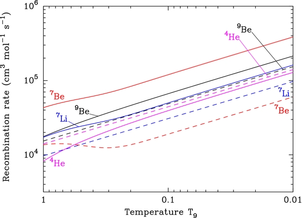
Figure 34. Rates for recombination of 7Be, 7Li, 9Be, and 4He with X− in the case of mX = 1000 GeV as a function of temperature. Solid lines show the recombination rates derived in this paper, while dashed lines show the rates adopted in the previous studies (see the text).
Download figure:
Standard image High-resolution image9.6.2. Case without 7BeX Decay
When the charged-current decay of 7BeX → 7Li+X0 is absent, the following reactions predominantly determine the abundance evolution of 7Be, 7Li, and 6Li: (1) 7Be(X−, γ)7BeX, (2) 7BeX(p, γ)8BX, (3) 7Li(X−, γ)7LiX, (4) 7LiX(p, 2α)X−, (5) 4He(X−, γ)4HeX, and (6) 4HeX(d, X−)6Li. We updated the recombination rates for (1), (3), (5), and also the resonant proton capture rate for (2). The rates for (4) and (6) are taken from the same reference (Kamimura et al. 2009) as adopted in the previous studies.
In the theoretical calculation of 7Li/H, the most important reactions are (1) and (2). The new recombination rate for (1) is about five times larger than the previous rate (Figure 34) at the recombination temperature of T9 ∼ 0.36 (Section 9.5.1). On the other hand, the adopted destruction rate for (2) for the WS40 model is about 2.7 times larger than the previous rate (Figure 5) at the destruction temperature T9 ∼ 0.3 (Figure 31). Because of increases in the two reaction rates, the effective rate for 7Be destruction (or reduction in the final 7Li/H value) becomes higher than the previous one.
Second, the observational constraint on the abundance of 7Li/H has been updated from 7Li/H  (95 % confidence limits; Ryan et al. 2000) to log(7Li/H) =−12 + (2.199 ± 0.086) (Sbordone et al. 2010). As a result, curves of d(7Li) = 2 correspond to different abundances: 7Li/H =3.16 × 10⁻¹⁰ in this study, while 7Li/H =2.46 × 10⁻¹⁰ in the previous studies. In this study, therefore, we need less destruction of 7Be to realize d(7Li) = 2.
Both the theoretical and observational improvements indicate that it is easier to reduce the primordial 7Li abundance to the level of d(7Li) = 2. The contours of d(7Li) therefore move left by a factor of about 20 in the parameter plane of Figure 32. In the parameter region around d(7Li) = 2, a partial destruction of 7Be is realized. In this region, the destruction rate of 7Be is proportional to the product of reaction rates (1) and (2). The factor of ∼20 can be explained by this proportionality and the difference in the destruction fraction of 7Be required from observations.
The 6Li/H abundance, on the other hand, is not much changed from that in the previous studies both theoretically and observationally. In the theoretical part, the most important reactions are (5) and (6). The new recombination rate of (5) is lower than the previous rate by only about 10% (Figure 34) at the recombination temperature T9 ∼ 0.1 (Figure 31). In the observational part, the constraint has been updated from 6Li/H =(7.1 ± 0.7) × 10−12 (the average of stars with 6Li detections in Asplund et al. 2006) to 6Li/H = (0.9 ± 4.3) × 10−12 (the least stringent 2σ upper limit from Lind et al. 2013). Curves of d(6Li) = 10 then correspond to 6Li/H =9.5 × 10⁻¹¹ in this study, and 6Li/H =7.1 × 10⁻¹¹ in the previous studies. These slight changes do not move the contour of d(6Li) = 10 much. The contour then moves left only by a factor of about 1.4.
The interesting parameter region for the 7Li reduction subsequently moves upper left. The constraint on the 7Li abundance is significantly changed while that on the 6Li abundance is not changed. The parameter region is therefore exclusively affected by the change of the 7Li contour. The minimum X− abundance required for the effective 7Li reduction is YX = 0.04 in this study. This value is only about four percent of the previous estimate YX ∼ 1 (Kusakabe et al. 2010).
9.6.3. Case with 7BeX Decay
When the charged-current decay of 7BeX → 7Li+X0 is operative, the 7Be destruction rate is determined only by (1) 7Be(X−, γ)7BeX since the 7BeX nucleus is assumed to be instantaneously destroyed.
In the theoretical calculation of 7Li/H, the new larger rate of (1) moves the contours of d(7Li) to the left by a factor of about five. The constraint on the 6Li/H abundance is the same as in the case without 7BeX decay. The interesting parameter region then moves to upper left because of the changes of the theoretical result and the observational constraint on the 7Li abundance. The minimum X− abundance required for the effective 7Li reduction is YX = 6 × 10⁻³ in this study. This value is about a factor of seven below that of the previous estimate YX ∼ 0.04 (Kusakabe et al. 2008).
10. SUMMARY
We have completed a new detailed study of the effects of a long-lived negatively CHAMP, i.e., X−, on BBN. The BBN model including the X− particle is motivated by the discrepancy between the 7Li abundances predicted in SBBN model and those inferred from spectroscopic observations of MPSs. In the BBN model including the X−, 7Be is destroyed via a recombination reaction with the X− followed by a radiative proton capture reaction, i.e., 7Be(X−, γ)7BeX(p, γ)8BX. Since the primordial 7Li abundance is mainly from the abundance of 7Be produced during BBN, this 7Be destruction leads to a reduction of the primordial 7Li abundance, and it can explain the observed abundances. In addition, 6Li is produced via the recombination of 4He and X− followed by a deuteron capture reaction, i.e., 4He(X−, γ)4HeX(d, X−)6Li. Although the effects of many possible reactions have been studied, the 9Be abundance is not significantly enhanced in this BBN model.
In this paper, we have also made a new study of the effects of uncertainties in the nuclear charge distributions on the binding energies of nuclei and X− particles, the reaction rates, and the resultant BBN. We also calculated new radiative recombination rates for 7Be, 7Li, 9Be, and 4He with an X− taking into account the contributions from many partial waves of the scattering states. We also suggest a new reaction of 9Be production that enhances the primordial 9Be abundance to a level that might be detectable in future observations of MPSs.
In detail, this work can be summarized as follows.
- 1.We assumed three shapes for the nuclear charge density, i.e., WS, Gaussian, and homogeneous sphere types which were parameterized to reproduce the experimentally measured rms charge radii. The potentials between the X− and nuclei were then derived by folding the Coulomb potential and the nuclear charge densities (Section 2). Binding energies for nuclei plus X− were calculated for the different nuclear charge densities and different masses of the X−, mX. Along with the binding energies of the GS X-nuclei, those of the first atomic excited states of 8B
 and 9B were derived since these states provide important resonances in the 7Be(p, γ)8BX and 8Be(p, γ)9BX reactions (Section 3). Resonant rates for radiative proton capture were then calculated. We found that the different charge distributions result in reaction rates that can differ by significant factors depending upon the temperature. This is because the rates depend on the resonance energies that are sensitive to relatively small changes in binding energies of X-nuclei caused by the different nuclear charge distributions (Section 4).
 - 2.We also calculated new precise rates for the radiative recombinations of 7Be, 7Li, 9Be, and 4He with an X− for four choices of the mass, mX. For that purpose, binding energies and wave functions of the respective X-nuclei were derived for several bound states. In the recombination process for 7Be and 7Li, bound states of the nuclear first excited states, 7Be* and 7Li*, with X− can operate as effective resonances. These resonant reaction rates as well as transition matrices, radiative decay widths of the resonances, and resonance energies were calculated using derived wave functions. For 9Be and 4He, however, there are no important resonances in the recombination processes since the resonance energies are much higher than the typical temperatures corresponding to the recombination epoch. (Section 5)
- 3.For the four nuclei 7Be, 7Li, 9Be, and 4He, we calculated continuum-state wave functions for l = 0 to 4, and nonresonant recombination rates for the respective partial waves of scattering states and bound states. It was found that the finite sizes of the nuclear charge distributions causes deviations in the bound and continuum wave functions compared to those derived assuming that nuclei are point charges. These deviations are larger for larger mX and for heavier nuclei with a larger charge. In addition, the effect of the finite charge distribution predominantly affects the wave functions for tightly bound states and those for scattering states with small angular momenta l. We found the important characteristics of the 7Be+X− recombination. That is, for the heavy X−, mX ≳ 100 GeV, the most important transition in the recombination is the d-wave → 2P. Transitions f-wave → 3D and d-wave → 3P are also more efficient than that for the GS formation. This fact is completely different from the formation of hydrogen-like electronic ions described by the point-charge distribution. In this case the transition p-wave → 1S is predominant. The same characteristics that the transition d-wave → 2P is most important was found for the recombinations of 7Li and 9Be. Since 4He is lighter and its charge is smaller than 7Li and 7, 9Be, the effect of a finite charge distribution is smaller. In the 4He recombination, therefore, the transition p-wave → 1S is dominant as in the case of a point-charge nucleus. Recombination rates for other nuclei were estimated using a simple Bohr atomic model formula (Section 5).
- 4.Our nonresonant rate for the 7Be(X−, γ)7BeX reaction with mX = 1000 GeV is more than six times larger than the previously estimated rate (Bird et al. 2008). This difference is caused by our treatment of many bound states and many partial waves for the scattering states (Section 5). This improvement in the rate provides an improved constraint on the X− particle properties (Section 9).
- 5.We have also suggested a new reaction for 9Be production, i.e., 7LiX(d, X−)9Be. We adopted an example reaction rate using the astrophysical S-factor for the reaction 7Li(d, nα)4He as a starting point (Section 6). This reaction was found to significantly enhance the primordial 9Be abundance from our BBN network calculation (Section 9).
- 6.Using the binding energies of X-nuclei calculated in Section 3, mass excesses of X-nuclei along with rates and Q-values for reactions involving the X− particle were calculated for four cases of mX. The reaction network included the β-decays of X-nuclei, nuclear reactions of X-nuclei and their inverse reactions. Q-values and reverse reaction coefficients were found to be heavily dependent on mX (Section 7). The X−-particle mass dependence of the Q-value is especially important for the resonant reaction 7BeX(p, γ)8BX (Section 9).
- 7.We constructed an updated BBN code that includes the new reaction rates derived in this paper (Section 8). BBN calculations based on this code were then shown for four cases of mX. It was found that the amounts of 7Be destruction depend significantly on the assumed charge distribution form of the 7Be nucleus for the mX = 1000 GeV case. Finally, we derived new most realistic constraints on the initial abundance and the lifetime of the X− particle. Parameter regions for the solution to the 7Li problem were identified for the respective mX cases. We also derived the expected primordial 9Be abundances predicted in the allowed parameter regions. The predicted 9Be abundances are larger than in the SBBN model, but smaller than the present observational upper limit from MPSs (Section 9).
- 8.Some discussion was also given for E1 transitions that simultaneously change both nuclear and atomic states of 7BeX and 7LiX. These are hindered because of the near orthogonality of the atomic and nuclear wave functions. It was suggested, however, that for exotic atoms composed of nuclei and an X− with mass much larger than the nucleon mass, this orthogonality in the atomic and nuclear wave functions can be somewhat broken. Such exotic atoms may, therefore, have large rates for E1 transitions that simultaneously change nuclear and atomic states (the Appendix).


We are grateful to Professor Masayasu Kamimura for discussion on the reaction cross sections. This work was supported by the National Research Foundation of Korea (grant Nos. 2012R1A1A2041974, 2014R1A2A2A05003548, 2012M7A1A2055605), and in part by Grants-in-Aid for Scientific Research of JSPS (24340060), and Scientific Research on Innovative Areas of MEXT (20105004). Work at the University of Notre Dame (G.J.M.) was supported by the U.S. Department of Energy under Nuclear Theory grant DE-FG02-95-ER40934.
APPENDIX: TRANSITIONS OF EXOTIC ATOMS THAT SIMULTANEOUSLY CHANGE BOTH NUCLEAR AND ATOMIC STATES
Here we discuss in detail the Type 3 transitions in the 7Be(X−, γ)7BeX reaction that was addressed in Section 5.1.
A.1. Electric Dipole Transition Rate
The reduced probability for a transition from an initial state (i) to a final state (f) is given by
where Ik, Mk, and  are the spins, the magnetic quantum numbers, and the wave functions, respectively, of state k for initial (i) and final (f) states, with μ = Mi − Mf. We consider the three-body system of α, 3He, and X− located at the position vectors
  for i = 1 (α), 2 (3He), and 3 (X−), respectively. This system has bound states of 7BeX. The system of 7LiX can be considered similarly to this system. The electric dipole (E1) operator is given by
  (E1, μ)
  where qi is the electric charge,
  is the distance from the origin to the position of particle i, and
  are the spherical surface harmonics.
A.2. Hindrance of the Matrix Element
The wave function describing atoms composed of a nucleus with A = 7 and a negatively CHAMP X− is approximately given by a product of functions of a 7Z nuclear state and a 7ZX atomic state, i.e.,
where  is the nuclear wave function for the two-body system of particles 1 and 2, with the spin jβ and magnetic quantum numbers mβ for β = 1 (for state i) and 2 (for state f).
  is the atomic wave function for the two-body system of particles (1+2)+3, with nk, lk, and mk the main, azimuthal, and magnetic quantum numbers, respectively. (jβmβlkmk|IkMk) is the Clebsch–Gordan coefficient for (β, k) =(1, i) and (2, f).

are Jacobi coordinates, where  is the mass of particle i. The atomic wave function is then simply given by
  for k = i and f.
One can consider transitions which change the atomic and nuclear states simultaneously. This type of transition proceeds from states (7Be )*a or 7Be
 to (7BeX)*a or 7BeX, where the initial states are atomic excited states or GS composed of the first nuclear excited state 7Be*(1/2−), and the final states are atomic excited states or GS of the nuclear GS 7Be(3/2−). We show that the E1 rates for such transitions are smaller than those for typical E1 allowed nuclear transitions. For simplicity, we approximately neglect the finite-size charge distributions of α and 3He, and assume that all three particles are point charges. Then, the electric dipole moment is given by
where  and qr are defined as coefficients of
  and
and  , respectively.
Using Equations (A2) and (A4), the matrix element in Equation (A1) can be rewritten as
The orthogonality of the wave functions satisfies the conditions of  and
and  = 0 if both the nuclear and atomic states change in the reaction. This E1 matrix element is thus found to be zero.
A.3. E1 Rate Enhanced by a Heavy X− Particle
Contrary to the approximate estimation described above, the E1 transition rate is not expected to vanish, although it is hindered compared to the E1 rate for allowed nuclear transitions. This is because particles can have charge distributions of finite size. In the present case, α and 3He have a finite charge distribution. We explain this effect by comparing the electronic ion, 7Be3 +, and the exotic ion of the massive X− particle, 7BeX.
Average radii of electronic ions composed of an electron and light nuclei are  while the average radii of nuclear wave functions for light nuclei are
  . Since the two radius scales are different from each other by a large factor, the atomic and nuclear wave functions can be separately considered for the following reason: (1) nuclear wave functions are not affected by the existence of the electrons which are far away from the nuclei, and (2) atomic wave functions are not affected by the nuclear charge distribution since the Coulomb potential between an electron and the nucleus does not depend on the nuclear charge distribution except at very small atomic radii r' comparable to the nuclear charge radius.
When the mass of the X− is larger than ∼1 GeV, however, the average radii of 7BeX atomic states approach  . This is roughly the same order of magnitude as the charge radius of the 7Be nucleus. At large nuclear radii, therefore, effects of the Coulomb forces by the X− particle are not completely negligible in nuclear wave functions. Nuclear wave functions then depend not only on the nuclear radii but also on atomic radii. In addition, at small atomic radii the effects of the finite nuclear charge distribution reflecting a nuclear cluster structure are not completely negligible in atomic wave functions. Atomic wave functions then depend not only on atomic radii but also on nuclear radii. Therefore, nuclear and atomic wave functions are not strictly orthogonal, and the E1 matrix element is finite.
It is physically interesting that rates for E1 transitions simultaneously changing nuclear and atomic states can be larger if the X− particle is heavier. The rates are expected to be large for not only the hypothetical X− particle predicted in beyond the standard model physics, but also known negatively charged heavy particles such as μ−, π−,  , and so on. For example, ordinary and radiative muon captures on a proton, in which the latter just corresponds to the recombination process in this work, were performed in TRIUMF (Jonkmans et al. 1996), but the theoretical interpretation is still under discussions (Cheoun et al. 2003).
In addition to the pure Coulomb force, spin-dependent interactions can exist between an X− particle and nuclear clusters if the X− particle has a spin. In this paper, we assumed a spinless X− particle. In general, however, spin dependent interactions can mix states of A + X− and A* + X− so that the overlap integrals can be non-zero (M. Kamimura 2013, private communication).
Footnotes
- 7
[A/B] =log (nA/nB) − log (nA/nB)☉, where ni is the number density of i and the subscript ☉ indicates the solar value for elements A and B.
- 8
7Be produced during the BBN is transformed into 7Li by electron capture in the epoch of the recombination of 7Be and electron much later than the BBN epoch. The primordial 7Li abundance is therefore the sum of abundances of 7Li and 7Be produced in BBN. In SBBN with the baryon-to-photon ratio inferred from WMAP, 7Li is produced mostly as 7Be during the BBN.
- 9
Throughout the paper, we use natural units, ℏ = c = kB = 1, for the reduced Planck constant ℏ, the speed of light c, and the Boltzmann constant kB. We use the usual notation 1(2,3)4 for a reaction 1 + 2 → 3 + 4.
- 10
In the RADCAP code, there was an error in the numerical value of π, which was corrected.
- 11
In Bird et al. (2008), the effect of direct capture to the state 7Be
(2S) is estimated in the extreme assumption that the 2S state lies above the threshold of 7Be+X− with a resonance energy of 10 keV (Equation (2.11) of Bird et al. 2008). However, a three-body calculation for the α+3He+X− system has confirmed that the 2S state is below the energy threshold, and thus not a resonance. The resonant rate without the effect of the 2S state, i.e., Equation (2.9) of Bird et al. (2008), should therefore be used (M. Kamimura 2008, private communication; Section 3.6 in Kamimura et al. 2009). - 12
It appears that Equation (31) of Bertulani (2003) has an error.
