

Abstract
Imaging the Universe during the first hundreds of millions of years remains one of the exciting challenges facing modern cosmology. Observations of the redshifted 21 cm line of atomic hydrogen offer the potential of opening a new window into this epoch. This will transform our understanding of the formation of the first stars and galaxies and of the thermal history of the Universe. A new generation of radio telescopes is being constructed for this purpose with the first results starting to trickle in. In this review, we detail the physics that governs the 21 cm signal and describe what might be learnt from upcoming observations. We also generalize our discussion to intensity mapping of other atomic and molecular lines.
Export citation and abstract BibTeX RIS
This article was invited by K Kirby.
1. Introduction
Our understanding of cosmology has matured significantly over the last 20 years. In that time, observations of the Universe from its infancy, 400 000 years after the Big Bang, through to the present day, some 13.7 billion years later, have given us a basic picture of how the Universe came to be the way it is today. Despite this progress much of the first billion years of the Universe, a period when the first stars and galaxies formed, is still an unobserved mystery.
Astronomers have an advantage over archaeologists in that the finite speed of light gives them a way of looking into the past. The further away an object is located the longer the light that it emits takes to reach an observer today. The image recorded at a telescope is therefore a picture of the object long ago when the light was first emitted. The construction of telescopes both on the Earth, such as Keck, Subaru and Very Large Telescope (VLT), and in space, such as the Hubble Space Telescope, has enabled astronomers to directly observe galaxies out to distances corresponding to a time when the Universe was a billion years old.
Added to this, observations at microwave frequencies reveal the cooling afterglow of the Big Bang. This cosmic microwave background (CMB) decoupled from the cosmic gas 400 000 years after the Big Bang when the Universe cooled sufficiently for protons and electrons to combine to form neutral hydrogen. Radiation from this time is able to reach us directly, providing a snapshot of the primordial Universe.
Despite current progress, connecting these two periods represents a considerable challenge. Our understanding of structure is based upon the observation of small perturbations in the temperature maps of the CMB. These indicate that the early Universe was inhomogeneous at the level of 1 part in 100 000. Over time the action of gravity causes the growth of these small perturbations into larger non-linear structures, which collapse to form sheets, filaments and halos. These non-linear structures provide the framework within which galaxies form via the collapse and cooling of gas until the density required for star formation is reached.
The theoretical picture is well established, but the middle phase is largely untested by observations. To improve on this astronomers are pursuing two main avenues of attack. The first is to extend existing techniques by building larger, more sensitive, telescopes at a variety of wavelengths. On the ground, there are plans for optical telescopes with an aperture diameter of 24–39 m—the Giant Magellan Telescope (GMT), the Thirty Meter Telescope (TMT) and the European Extremely Large Telescope (E-ELT)—that would be able to detect an individual galaxy out to redshifts z > 10. In space, the James Webb Space Telescope (JWST) will operate at infrared wavelengths and potentially image some of the first galaxies at z ∼ 10–15. Other efforts involve the Atacama Large Millimeter/Submillimeter Array (ALMA), which will observe the molecular gas that fuels star formation in galaxies during reionization (z = 8 − 10). These efforts target individual galaxies although the objects of interest are far enough away that only the brightest sources may be seen.
This review focuses on an alternative approach based upon making observations of the redshifted 21 cm line of neutral hydrogen. This 21 cm line is produced by the hyperfine splitting caused by the interaction between electron and proton magnetic moments. Hydrogen is ubiquitous in the Universe, amounting to ∼75% of the gas mass present in the intergalactic medium (IGM). As such, it provides a convenient tracer of the properties of that gas and of major milestones in the first billion years of the Universe's history.
The 21 cm line from gas during the first billion years after the Big Bang redshifts to radio frequencies 30–200 MHz making it a prime target for a new generation of radio interferometers currently being built. These instruments, such as the Murchison Widefield Array (MWA), the LOw Frequency ARray (LOFAR), the Precision Array to Probe the Epoch of Reionization (PAPER), the 21 cm Array (21CMA) and the Giant Meter-wave Radio Telescope (GMRT), seek to detect the radio fluctuations in the redshifted 21 cm background arising from variations in the amount of neutral hydrogen. Next generation instruments (e.g. the Square Kilometre Array (SKA)) will be able to go further and might make detailed maps of the ionized regions during reionization and measure properties of hydrogen out to z = 30. These observations constrain the properties of the IGM and by extension the cumulative impact of light from all galaxies, not just the brightest ones. In combination with direct observations of the sources they provide a powerful tool for learning about the first stars and galaxies. They will also provide information about active galactic nuclei (AGNs), such as quasars, by observing the ionized bubbles surrounding individual AGNs.
In addition to learning about galaxies and reionization, 21 cm observations have the potential to inform us about fundamental physics too. Part of the signal traces the density field giving information about neutrino masses and the initial conditions from the early epoch of cosmic inflation in the form of the power spectrum. However spin-temperature fluctuations driven by astrophysics also contribute to the signal. Getting at this cosmology is a challenge, since the astrophysical effects must be understood before cosmology can be disentangled. One possibility is to exploit the effect of redshift space distortions, which also produce 21 cm fluctuations but directly trace the density field. In the long term, 21 cm cosmology may allow precision measurements of cosmological parameters by opening up large volumes of the Universe to observation.
The goal of this review is to summarize the physics that determines the 21 cm signal, along with a comprehensive overview of related astrophysics. Figure 1 provides a summary of the 21 cm signal showing the key features of the signal with the relevant cosmic time, frequency and redshift scales indicated. The earliest period of the signal arises in the period after thermal decoupling of the ordinary matter (baryons) from the CMB, so that the gas is able to cool adiabatically with the expansion of the Universe. In these cosmic 'Dark Ages', before the first stars have formed, the first structures begin to grow from the seed inhomogeneties thought to be produced by quantum fluctuations during inflation. The cold gas can be seen in a 21 cm absorption signal, which has both a mean value (shown in the bottom panel) and fluctuations arising from variation in density (shown in the top panel). Once the first stars and galaxies form, their light radically alters the properties of the gas. Scattering of Lyα photons leads to a strong coupling between the excitation of the 21 cm line spin states and the gas temperature. Initially, this leads to a strong absorption signal that is spatially varying due to the strong clustering of the rare first generation of galaxies. Next, the x-ray emission from these galaxies heats the gas leading to a 21 cm emission signal. Finally, UV photons ionize the gas producing dark holes in the 21 cm signal within regions of ionized bubbles surrounding groups of galaxies. Eventually all of the hydrogen gas, except for that in a few dense pockets, is ionized.

Figure 1. The 21 cm cosmic hydrogen signal. (a) Time evolution of fluctuations in the 21 cm brightness from just before the first stars formed through to the end of the reionization epoch. This evolution is pieced together from redshift slices through a simulated cosmic volume [1]. Coloration indicates the strength of the 21 cm brightness as it evolves through two absorption phases (purple and blue), separated by a period (black) where the excitation temperature of the 21 cm hydrogen transition decouples from the temperature of the hydrogen gas, before it transitions to emission (red) and finally disappears (black) owing to the ionization of the hydrogen gas. (b) Expected evolution of the sky-averaged 21 cm brightness from the 'Dark Ages' at redshift 200 to the end of reionization, sometime before redshift 6 (solid curve indicates the signal; dashed curve indicates Tb = 0). The frequency structure within this redshift range is driven by several physical processes, including the formation of the first galaxies and the heating and ionization of the hydrogen gas. There is considerable uncertainty in the exact form of this signal, arising from the unknown properties of the first galaxies. Reproduced with permission from [2]. Copyright 2010 Nature Publishing Group.
Download figure:
Standard imageThroughout this review, we will make reference to parameters describing the standard ΛCDM cosmology. These describe the mass densities in non-relativistic matter Ωm = 0.26, dark energy ΩΛ = 0.74 and baryons Ωb = 0.044 as a fraction of the critical mass density. We further parametrize the Hubble parameter H0 = 100h km s−1 Mpc−1 with h = 0.74. Finally, the spectrum of fluctuations is described by a logarithmic slope or 'tilt' nS = 0.95, and the variance of matter fluctuations today smoothed on a scale of 8h−1 Mpc is σ8 = 0.8. The values quoted are indicative of those found by the latest measurements [3].
The layout of this review is as follows. We first discuss the basic atomic physics of the 21 cm line in section 2. In section 3, we turn to the evolution of the sky-averaged 21 cm signal and the feasibility of observing it. In section 4 we describe 3D 21 cm fluctuations, including predictions from analytical and numerical calculations. After reionization, most of the 21 cm signal originates from cold gas in galaxies (which is self-shielded from the background of ionizing radiation). In section 5 we describe the prospects for intensity mapping (IM) of this signal as well as using the same technique to map the cumulative emission of other atomic and molecular lines from galaxies without resolving the galaxies individually. The 21 cm forest that is expected against radio-bright sources is described in section 6. Finally, we conclude with an outlook for the future in section 7.
We direct interested readers to a number of other worthy reviews on the subject. Reference [4] provides a comprehensive overview of the entire field, and [5] takes a more observationally orientated approach focusing on the near term observations of reionization.
2. Physics of the 21 cm line of atomic hydrogen
2.1. Basic 21 cm physics
As the most common atomic species present in the Universe, hydrogen is a useful tracer of local properties of the gas. The simplicity of its structure—a proton and electron—belies the richness of the associated physics. In this review, we will be focusing on the 21 cm line of hydrogen, which arises from the hyperfine splitting of the 1S ground state due to the interaction of the magnetic moments of the proton and the electron. This splitting leads to two distinct energy levels separated by ΔE = 5.9 × 10⁻⁶ eV, corresponding to a wavelength of 21.1 cm and a frequency of 1420 MHz. This frequency is one of the most precisely known quantities in astrophysics having been measured to great accuracy from studies of hydrogen masers [6].
The 21 cm line was theoretically predicted by van de Hulst in 1942 [7] and has been used as a probe of astrophysics since it was first detected by Ewen and Purcell in 1951 [8]. Radio telescopes look for emission by warm hydrogen gas within galaxies. Since the line is narrow with a well measured rest frame frequency it can be used in the local Universe as a probe of the velocity distribution of gas within our galaxy and other nearby galaxies. The 21 cm rotation curves are often used to trace galactic dynamics. Traditional techniques for observing 21 cm emission have only detected the line in relatively local galaxies, although the 21 cm line has been seen in absorption against radio-loud background sources from individual systems at redshifts z ≲ 3 [9, 10]. A new generation of radio telescopes offers the exciting prospect of using the 21 cm line as a probe of cosmology.
In passing, we note that other atomic species show hyperfine transitions that may be useful in probing cosmology. Of particular interest are the 8.7 GHz hyperfine transition of 3He+ [11, 12], which could provide a probe of helium reionization, and the 92 cm deuterium analogue of the 21 cm line [13]. The much lower abundance of deuterium and 3He compared with neutral hydrogen makes it more difficult to take advantage of these transitions.
In cosmological contexts the 21 cm line has been used as a probe of gas along the line of sight to some background radio source. The detailed signal depends upon the radiative transfer through gas along the line of sight. We recall the basic equation of radiative transfer for the specific intensity Iν (per unit frequency ν) in the absence of scattering along a path described by coordinate s [14]:

where absorption and emission by gas along the path are described by the coefficients αν and jν, respectively.
To simplify the discussion, we will work in the Rayleigh–Jeans limit, appropriate here since the relevant photon frequencies ν are much smaller than the peak frequency of the CMB blackbody. This allows us to relate the intensity Iν to a brightness temperature T by the relation Iν = 2kBTν2/c2, where c is the speed of light and kB is Boltzmann's constant. We will also make use of the standard definition of the optical depth
 . With this we may rewrite (1) to give the radiative transfer for light from a background radio source of brightness temperature TR along the line of sight through a cloud of optical depth τν and uniform excitation temperature Tex so that the observed temperature
 at a frequency ν is given by

The excitation temperature of the 21 cm line is known as the spin temperature TS. It is defined through the ratio between the number densities ni of hydrogen atoms in the two hyperfine levels (which we label with a subscript 0 and 1 for the 1S singlet and 1S triplet levels, respectively)

where g1/g0 = 3 is the ratio of the statistical degeneracy factors of the two levels, and T⋆ ≡ hc/kλ21 cm = 0.068 K.
With this definition, the optical depth of a cloud of hydrogen is then

where n0 = nH/4 with nH being the hydrogen density, and we have denoted the 21 cm cross-section as σ(ν) = σ0φ(ν), with σ0 ≡ 3c2A10/8πν2, where A10 = 2.85 × 10⁻¹⁵ s−1 is the spontaneous decay rate of the spin–flip transition, and the line profile is normalized so that ∫φ(ν) dν = 1. To evaluate this expression we need to find the column length as a function of frequency s(ν) to determine the range of frequencies dν over the path ds that correspond to a fixed observed frequency νobs. This can be done in one of two ways: by relating the path length to the cosmological expansion ds = −c dz/(1 + z)H(z) and the redshifting of light to relate the observed and emitted frequencies νobs = νem/(1 + z) or assuming a linear velocity profile locally v = (dv/ds)s (the well-known Sobolev approximation [15]) and using the Doppler law νobs = νem(1 − v/c) self-consistently to
 . Since the latter case describes the well-known Hubble law in the absence of peculiar velocities these two approaches give identical results for the optical depth. The latter picture brings out the effect of peculiar velocities that modify the local velocity–frequency conversion.
The optical depth of this transition is small at all relevant redshifts, yielding a differential brightness temperature


Here
 is the neutral fraction of hydrogen, δb is the fractional overdensity in baryons and the final term arises from the velocity gradient along the line of sight ∂rvr.
The key to the detectability of the 21 cm signal hinges on the spin temperature. Only if this temperature deviates from the background temperature, will a signal be observable. Much of this review will focus on the physics that determines the spin temperature and how spatial variation in the spin temperature conveys information about astrophysical sources.
Three processes determine the spin temperature: (i) absorption/emission of 21 cm photons from/to the radio background, primarily the CMB; (ii) collisions with other hydrogen atoms and with electrons; and (iii) resonant scattering of Lyα photons that cause a spin–flip via an intermediate excited state. The rate of these processes is fast compared with the deexcitation time of the line, so that to a very good approximation the spin temperature is given by the equilibrium balance of these effects. In this limit, the spin temperature is given by [16]

where Tγ is the temperature of the surrounding bath of radio photons, typically set by the CMB so that Tγ = TCMB; Tα is the color temperature of the Lyα radiation field at the Lyα frequency and is closely coupled to the gas kinetic temperature TK by recoil during repeated scattering and xc, xα are the coupling coefficients due to atomic collisions and scattering of Lyα photons, respectively. The spin temperature becomes strongly coupled to the gas temperature when xtot ≡ xc+xα≳1 and relaxes to Tγ when xtot ≪ 1.
Two types of background radio sources are important for the 21 cm line as a probe of astrophysics. Firstly, we may use the CMB as a radio background source. In this case, TR = TCMB and the 21 cm feature is seen as a spectral distortion to the CMB blackbody at appropriate radio frequencies (since fluctuations in the CMB temperature are small δTCMB ∼ 10−5 the CMB is effectively a source of uniform brightness). The distortion forms a diffuse background that can be studied across the whole sky in a similar way to CMB anisotropies. Observations at different frequencies probe different spherical shells of the observable Universe, so that a 3D map can be constructed. This is the main subject of section 4.
The second situation uses a radio-loud point source, for example a radio-loud quasar, as the background. In this case, the source will always be much brighter than the weak emission from diffuse hydrogen gas, TR ≫ TS, so that the gas is seen in absorption against the source. The appearance of lines from regions of neutral gas at different distances to the source leads to a 'forest' of lines known as the '21 cm forest' in analogy to the Lyα forest. The high brightness of the background source allows the 21 cm forest to be studied with high frequency resolution so probing small-scale structures (∼kpc) in the IGM. For useful statistics, many lines of sight to different radio sources are required, making the discovery of high redshift radio sources a priority. We leave discussion of the 21 cm forest to section 6.
Note that we have a number of different quantities with units of temperature, many of which are not true thermodynamic temperatures. TR and δTb are measures of radio intensity. TS measures the relative occupation numbers of the two hyperfine levels. Tα is a colour temperature describing the photon distribution in the vicinity of the Lyα transition. Only the CMB blackbody temperature TCMB and TK are genuine thermodynamic temperatures.
2.2. Collisional coupling
Collisions between different particles may induce spin–flips in a hydrogen atom and dominate the coupling in the early Universe where the gas density is high. Three main channels are available: collisions between two hydrogen atoms and collisions between a hydrogen atom and an electron or a proton. The collisional coupling for a species i is [4, 16]

where C10 is the collisional excitation rate and
 is the specific rate coefficient for spin deexcitation by collisions with species i (in units of cm3 s−1).
The total collisional coupling coefficient can be written as

where
 is the scattering rate between hydrogen atoms,
 is the scattering rate between electrons and hydrogen atoms and
 is the scattering rate between protons and hydrogen atoms.
The collisional rates require a quantum mechanical calculation. Values for
have been tabulated as a function of Tk [17, 18], the scattering rate between electrons and hydrogen atoms
was considered in [19] and the scattering rate between protons and hydrogen atoms
was considered in [20]. Useful fitting functions exist for these scattering rates: the H–H scattering rate is well fit in the range 10 K < TK < 103 K by
 [21]; and the e–H scattering rate is well fit by
![$\log(\kappa^{\rm eH}_{1-0}/{\rm cm^3\,s^{-1}})=-9.607+0.5\log T_{\rm K}\times\exp[-(\log T_{\rm K})^{4.5}/1800]$](https://content.cld.iop.org/journals/0034-4885/75/8/086901/revision1/rpp295494ieqn010.gif) for T ⩽ 104 K and
for T ⩽ 104 K and
 [22].
[22].
During the cosmic Dark Ages, where the coupling is dominated by collisional coupling the details of the process become important. For example, the above calculations make use of the assumption that the collisional cross-sections are independent of velocity; the actual velocity dependance leads to a non-thermal distribution for the hyperfine occupation [23]. This effect can lead to a suppression of the 21 cm signal at the level of 5%, which although small is still important from the perspective of using the 21 cm signal from the Dark Ages for precision cosmology.
2.3. Wouthuysen–Field effect
For most of the redshifts that are likely to be observationally probed in the near future collisional coupling of the 21 cm line is inefficient. However, once star formation begins, resonant scattering of Lyα photons provides a second channel for coupling. This process is generally known as the Wouthuysen–Field effect [16, 24] and is illustrated in figure 2, which shows the hyperfine structure of the hydrogen 1S and 2P levels. Suppose that hydrogen is initially in the hyperfine singlet state. Absorption of a Lyα photon will excite the atom into either of the central 2P hyperfine states (the dipole selection rules ΔF = 0, 1 and no F = 0 → 0 transitions make the other two hyperfine levels inaccessible). From here emission of a Lyα photon can relax the atom to either of the two ground state hyperfine levels. If relaxation takes the atom to the ground level triplet state then a spin–flip has occurred. Hence, resonant scattering of Lyα photons can produce a spin–flip.

Figure 2. Left panel: hyperfine structure of the hydrogen atom and the transitions relevant for the Wouthuysen–Field effect [25]. Solid line transitions allow spin–flips, while dashed transitions are allowed but do not contribute to spin–flips. Right panel: illustration of how atomic cascades convert Lyn photons into Lyα photons. Reproduced with permission from [25]. Copyright 2006 Wiley.
Download figure:
Standard imageThe physics of the Wouthuysen–Field effect is considerably more subtle than this simple description would suggest. We may write the coupling as

where Pα is the scattering rate of Lyα photons. Here we have related the scattering rate between the two hyperfine levels to Pα using the relation P01 = 4Pα/27, which results from the atomic physics of the hyperfine lines and assumes that the radiation field is constant across them [26].
The rate at which Lyα photons scatter from a hydrogen atom is given by

where σν ≡ χαφα(ν) is the local absorption cross-section, χα ≡ (πe2/mec)fα is the oscillation strength of the Lyα transition, φα(ν) is the Lyα absorption profile and Jν(ν) is the angle-averaged specific intensity of the background radiation field (by number).
Making use of this expression, we can express the coupling as

where Jα is the specific flux evaluated at the Lyα frequency. Here we have introduced
 , with J∞ being the flux away from the absorption feature, as a correction factor of order unity to describe the detailed structure of the photon distribution in the neighbourhood of the Lyα resonance.
Equation (13) can be used to calculate the critical flux required to produce xα = Sα. We rewrite (13) as
 , where
![$J_\alpha^{\rm C}\equiv1.165\times10^{10}[(1+z)/20]{\rm \,cm^{-2}\,s^{-1}\,Hz^{-1}\,sr^{-1}}$](https://content.cld.iop.org/journals/0034-4885/75/8/086901/revision1/rpp295494ieqn014.gif) . The critical flux can also be expressed in terms of the number of Lyα photons per hydrogen atom
. The critical flux can also be expressed in terms of the number of Lyα photons per hydrogen atom
![$J_\alpha^{\rm C}/n_{\rm H}=0.0767[(1+z)/20]^{-2}$](https://content.cld.iop.org/journals/0034-4885/75/8/086901/revision1/rpp295494ieqn015.gif) . In practice, this condition is easy to satisfy once star formation begins.
. In practice, this condition is easy to satisfy once star formation begins.
The above physics couples the spin temperature to the colour temperature of the radiation field, which is a measure of the shape of the radiation field as a function of frequency in the neighbourhood of the Lyα line defined by [27]

where nν = c2Jν/2ν2 is the photon occupation number. Some care must to taken with this definition; other definitions that do not obey detailed balance can be found in the literature.
Typically, Tc ≈ TK, because in most cases of interest the optical depth to Lyα scattering is very large leading to a large number of scatterings of Lyα photons that bring the radiation field and the gas into local equilibrium for frequencies near the line centre [28]. At the level of microphysics this relation occurs through the process of scattering Lyα photons in the neighbourhood of the Lyα resonance, which leads to a distinct feature in the frequency distribution of photons. Without going into the details, one can understand the formation of this feature in terms of the 'flow' of photons in frequency. Redshifting with the cosmic expansion leads to a flow of photons from high to low frequency at a fixed rate. As photons flow into the Lyα resonance they may scatter to larger or smaller frequencies. Since the cross-section is symmetric, one would expect the net flow rate to be preserved. However, each time a Lyα photon scatters from a hydrogen atom it will lose a fraction of its energy hν/mpc2 due to the recoil of the atom. This loss of energy increases the flow to lower energy and leads to a deficit of photons close to line centre. As this feature develops scattering redistributes photons leading to an asymmetry about the line. This asymmetry is exactly that required to bring the distribution into local thermal equilibrium with Tc ≈ TK.
The shape of this feature determines Sα and, since recoils source an absorption feature, ensures Sα ⩽ 1. At low temperatures, recoils have more of an effect and the suppression of the Wouthuysen–Field effect is most pronounced. If the IGM is warm then this suppression becomes negligible [29–32]. The above discussion has neglected processes whereby the distribution of photons is changed by spin-exchanges. Including this complicates the determination of TS and Tc considerably since they must then be iterated to find a self-consistent solution for the level- and photon-populations [30]. However, the effect of spin–flips on the photon distribution is small ≲10%.
A useful approximation for Sα is outlined in [31]: Sα ≈ exp(−1.79α), where α ≡ η (3a/2πγ)1/3, a = Γ/(4πΔνD), Γ the inverse lifetime of the upper 21 cm level, ΔνD/ν0 = (2kBTK/mc2)1/2 is the Doppler parameter, ν0 the line centre frequency,
 and
and
 is the mean frequency drift per scattering due to recoil, which is accurate at the 5% level provided that TK ≳ 1 K and the Gunn–Peterson optical depth τGP is large.
In the astrophysical context, we will primarily be interested in photons redshifting into the Lyα resonance from frequencies below the Lyβ resonance. In addition, Lyα photons can be produced by atomic cascades from photons redshifting into higher Lyman series resonances. These atomic cascades are illustrated in figure 2, where the probability of converting a Lyn photon into a Lyα photon is set by the atomic rate coefficients and can be found in tabular form in [25, 30]. For large n, approximately 30% conversion is typical. These photons are injected into the Lyα line rather than being redshifted from outside of the line. This changes their contribution to the Wouthuysen–Field coupling since the photon distribution is now one-sided. Similar processes to those described above apply to the redistribution of these photons, and they can lead to an important amplification of the Lyα flux.
This discussion gives a sense of some of the subtleties that go into determining the strength of the Lyα coupling. These effects can modify the 21 cm signal at the ∼10% level, which will be important as observations begin to detect 21 cm fluctuations. At this stage, it appears that the underlying atomic physics is understood, although the details of Lyα radiative transfer still requires some work.
3. Global 21 cm signature
3.1. Outline
Next we examine the cosmological context of the 21 cm signal. We may express the 21 cm brightness temperature as a function of four variables Tb = Tb(TK, xi, Jα, nH), where xi is the volume-averaged ionized fraction of hydrogen. In calculating the 21 cm signal, we require a model for the global evolution of and fluctuations in these quantities. Before looking at the evolution of the signal quantitatively, we will first outline the basic picture to delineate the most important phases.
An important feature of Tb is that its dependence on each of these quantities saturates at some point, for example once the Lyα flux is high enough the spin and kinetic gas temperatures become tightly coupled and further variation in Jα becomes irrelevant to the details of the signal. This leads to conceptually separate regimes where variation in only one of the variables dominating fluctuations in the signal. These different regimes can be seen in figure 1 and are shown in schematic form in figure 3 for clarity. We now discuss each of these phases in turn.
- 200 ≲ z ≲ 1100. The residual free electron fraction left after recombination allows Compton scattering to maintain thermal coupling of the gas to the CMB, setting TK = Tγ. The high gas density leads to effective collisional coupling so that TS = Tγ and we expect
 and no detectable 21 cm signal.
 - 40 ≲ z ≲ 200. In this regime, the gas cools adiabatically so that TK ∝ (1 + z)2 leading to TK < Tγ and collisional coupling sets TS < Tγ, leading to
and an early absorption signal. At this time, Tb fluctuations are sourced by density fluctuations, potentially allowing the initial conditions to be probed [23, 33].
- z⋆ ≲ z ≲ 40. As the expansion continues, decreasing the gas density, collisional coupling becomes ineffective and radiative coupling to the CMB sets TS = Tγ, and there is no detectable 21 cm signal.
-
. Once the first sources switch on at z⋆, they emit both Lyα photons and x-rays. In general, the emissivity required for Lyα coupling is significantly less than that for heating TK above Tγ. We therefore expect a regime where the spin temperature is coupled to cold gas so that TS ∼ TK < Tγ and there is an absorption signal. Fluctuations are dominated by density fluctuations and variation in the Lyα flux [25, 34, 35]. As further star formation occurs the Lyα coupling will eventually saturate (xα ≫ 1), so that by a redshift zα the gas will everywhere be strongly coupled.
-
. After Lyα coupling saturates, fluctuations in the Lyα flux no longer affect the 21 cm signal. By this point, heating becomes significant and gas temperature fluctuations source Tb fluctuations. While TK remains below Tγ we see a 21 cm signal in absorption, but as TK approaches Tγ hotter regions may begin to be seen in emission. Eventually by a redshift zh the gas will be heated everywhere so that
.
-
. After the heating transition, TK > Tγ and we expect to see a 21 cm signal in emission. The 21 cm brightness temperature is not yet saturated, which occurs at zT, when TS ∼ TK ≫ Tγ. By this time, the ionization fraction has likely risen above the per cent level. Brightness temperature fluctuations are sourced by a mixture of fluctuations in ionization, density and gas temperature.
-
. Continued heating drives TK ≫ Tγ at zT and temperature fluctuations become unimportant. TS ∼ TK ≫ Tγ and the dependence on TS may be neglected in equation (7), which greatly simplifies analysis of the 21 cm power spectrum [36]. By this point, the filling fraction of H ɪɪ regions probably becomes significant and ionization fluctuations begin to dominate the 21 cm signal [37].
-
. After reionization, any remaining 21 cm signal originates primarily from collapsed islands of neutral hydrogen (damped Lyα systems).


Figure 3. Cartoon of the different phases of the 21 cm signal. The signal transitions from an early phase of collisional coupling to a later phase of Lyα coupling through a short period where there is little signal. Fluctuations after this phase are dominated successively by spatial variation in the Lyα, x-ray and ionizing UV radiation backgrounds. After reionization is complete there is a residual signal from neutral hydrogen in galaxies.
Download figure:
Standard imageMost of these epochs are not sharply defined, and so there could be considerable overlap between them. In fact, our ignorance of early sources is such that we cannot definitively be sure of the sequence of events. The above sequence of events seems most likely and can be justified on the basis of the relative energetics of the different processes and the probable properties of the sources. We will discuss this in more detail as we quantify the evolution of the sources.
Perhaps the largest uncertainty lies in the ordering of zα and zh. Reference [38] explores the possibility that zh > zα, so that x-ray preheating allows collisional coupling to be important before the Lyα flux becomes significant. Simulations of the very first mini-quasar [21, 39] also probe this regime and show that the first luminous x-ray sources can have a great impact on their surrounding environment. We note that these studies ignored Lyα coupling, and that an x-ray background may generate significant Lyα photons [35], as we discuss in section 3.5. Additionally, while these authors looked at the case where the production of Lyα photons was inefficient, one can consider the case where heating is much more efficient. This can be the case where weak shocks raise the IGM temperature very early on [40] or if exotic particle physics mechanisms such as dark matter annihilation are important. Clearly, there is still considerable uncertainty in the exact evolution of the signal making the potential implications of measuring the 21 cm signal very exciting.
3.2. Evolution of global signal
Having outlined the evolution of the signal qualitatively, we will turn to the details of making quantitative predictions. In calculating the 21 cm signal it will help us to treat the IGM as a two phase medium. Initially, the IGM is composed of a single mostly neutral phase left over after recombination. This phase is characterized by a gas temperature TK and a small fraction of free electrons xe. This is the phase that generates the 21 cm signal.
Once galaxy formation begins, energetic UV photons ionize H ɪɪ regions surrounding, first individual galaxies and then clusters of galaxies. These UV photons have a very short mean free path in a neutral medium leading to the ionized H ɪɪ regions having a very sharp boundary (although the boundary can be softened if the ionizing photons are particularly hard [41]). We may therefore treat the ionized H ɪɪ bubbles as a second phase in the IGM characterized by a volume filling fraction xi (provided that the free electron fraction is small xi is approximately the mean ionization fraction). We will assume that these bubbles are fully ionized and that the temperature inside the bubbles is fixed at
 determining the collisional recombination rate inside these bubbles. Since the photons that redshift into the Lyα resonance initially have long mean free paths, we may treat the Lyα flux Jα as being the same in both phases (although in practice, since there is no 21 cm signal from the fully ionized bubbles, it is only the Lyα flux in the mostly neutral phase that matters). To determine the 21 cm signal at a given redshift, we must calculate the four quantities xi, xe, TK and Jα. We begin by describing the evolution of the gas temperature TK,

Here, the first term accounts for adiabatic cooling of the gas due to the cosmic expansion while the second term accounts for other sources of heating/cooling j with  j the heating rate per unit volume for the process j.
Next, we consider the volume filling fraction xi and the ionization of the neutral IGM xe


In these expressions, we define Λi to be the rate of production of ionizing photons per unit time per baryon applied to H ɪɪ regions, Λe is the equivalent quantity in the bulk of the IGM, αA = 4.2 × 10⁻¹³ cm3 s−1 is the case-A recombination coefficient at T = 104 K, αB(T) is the case-B recombination rate (whose temperature dependence can be obtained from [42]), and
 is the clumping factor.
Superficially these look the same, since in each case the ionization rate is a balance between ionizations and recombinations. The main distinction lies in the manner in which we treat the recombinations. In the fully ionized bubbles, recombinations occur in those dense clumps of material capable of self-shielding against ionizing radiation. These overdense regions will have a locally enhanced recombination rate, making it important to account for the inhomogeneous distribution of matter through the clumping factor C. Since recombinations will occur on the edge of these neutral clumps, secondary photons produced by the recombinations will likely be absorbed inside the clumps rather than in the mean IGM, justifying the use of case-A recombination [43]. In contrast, recombinations in the bulk of the neutral IGM will occur at close to mean density in gas with temperature TK. Here recombination radiation will be absorbed in the IGM, so we must use case-B recombination. By keeping track of this carefully our evolution matches that of RECFAST [42].
This two phase approximation will eventually break down should xe become close to unity, indicating that most of the IGM has been ionized and that there is no clear distinction between ionized bubbles and a neutral bulk IGM. In most of our models, xe remains small until the end of reionization making this a reasonable approximation.
3.3. Growth of H ɪɪ regions
The growth of ionized H ɪɪ regions is governed by the interplay between ionization and recombination, both of which contain considerable uncertainties. We may write the ionization rate per hydrogen atom as

with Nion being the number of ionizing photons per baryon produced in stars, fesc the fraction of ionizing photons that escape the host halo and AHe a correction factor for the presence of helium. Here
 is the star-formation rate (SFR) density as a function of redshift, which is still poorly known observationally. For a present-day initial mass function of stars, Nion ∼ 4 × 10³, whereas for very massive (>102M⊙) stars of primordial composition, Nion ∼ 105 [44, 45].
We model the SFR as tracking the collapse of matter, so that we may write the SFR per (comoving) unit volume

where
 is the cosmic mean baryon density today and f⋆ is the fraction of baryons converted into stars. This formalism is appropriate for z ≳ 10, as at later times star formation as a result of mergers becomes important.
With these assumptions, we may rewrite the ionization rate per hydrogen atom as

where fcoll(z) is the fraction of gas inside collapsed objects at z and the ionization efficiency parameter ζ is given by

This model for xi is motivated by a picture of H ɪɪ regions expanding into neutral hydrogen [46]. In calculating fcoll, we use the Sheth–Tormen [47] mass function dn/dm and determine a minimum mass mmin for collapse by requiring the virial temperature Tvir ⩾ 104 K, appropriate for cooling by atomic hydrogen. Decreasing this minimum galaxy mass, say to the virial temperature corresponding to molecular hydrogen cooling (∼300 K), will allow star formation to occur at earlier times, shifting the features that we describe in redshift.
The sources of ionizing photons in the early Universe are believed to have been primarily galaxies. However, the properties of these galaxies are currently only poorly constrained. Recent observations with the Hubble Space Telescope provide some of the best constraints on early galaxy formation. Faint galaxies are identified as being at high redshift using a 'Lyα dropout technique' where a naturally occurring break in the galaxy spectrum at the Lyα wavelength 1216 Å is seen in different colour filters as a galaxy is redshifted. So far, galaxies at redshifts up to z ∼ 10 have been found providing information on the sources of reionization. There are unfortunately considerable limitations on the existing surveys owing to their small sky coverage, which makes it unclear whether those galaxies seen are properly representative, and the limited frequency coverage. Even more problematic for our purposes is that the optical frequencies at which the galaxies are seen do not correspond to the UV photons that ionize the IGM. Our limited understanding of the mass distribution of the emitting stars introduces an uncertainty in the number of ionizing photons per baryon Nion is emitted by galaxies. There is also considerable uncertainty in the fraction of ionizing photons fesc that escape the host galaxy to ionize the IGM.
The recombination rate is primarily important at late times once a significant fraction of the volume has already been ionized. At this stage, dense clumps within an ionized bubble can act as sinks of ionizing photons slowing or even stalling further expansion of the bubble. The degree to which gas resides in these dense clumps is an important uncertainty in modelling reionization. Important hydrodynamic effects, such as the evaporation of gas from a halo as a result of photoionization heating [48], can significantly modify the clumping factor.
A simple model for the clumping factor [43] assumes that the Universe will be fully ionized up to some critical overdensity Δc. If the probability distribution for the gas density PV(Δ) is specified, we may then write the clumping factor as

The quantity PV(Δ) can be modelled analytically starting from a consideration of behaviour of low density voids and accounting for Gaussian initial conditions. The analytic form resembles that of a Gaussian with a power law tail [43] and can be measured from simulations [49]. To accurately capture the clumping one should self-consistently perform a full hydrodynamical simulation of reionization, since thermal feedback can modify the gas density distribution [48].
To set the critical density Δc, we account for the patchy nature of reionization, which proceeds via the expansion and overlap of ionized bubbles [50]. The size of bubbles will become limited if the mean free path of ionized photons becomes shorter than the size of the bubble, for example if the bubble contains many small self-shielded absorbers. The mean free path of ionizing photons can be related to the underlying density field as

Here λ0 is an unknown normalization constant that was found by [43] in the context of simulations at z = 2–4 to be well fit by λ0H(z) = 60 km s−1. This scaling relationship is likely to be very approximate, but we make use of it for convenience. With this we can fix Δi within an ionized bubble by setting the relevant Rb = λi(Δc). We then average the clumping factor over the distribution of bubble sizes (discussed in more details later) to get the mean clumping factor.
3.4. Heating and ionization
To determine the heating rate, we must integrate equation (15) and therefore we must specify which heating mechanisms are important. At high redshifts, the dominant mechanism is Compton heating of the gas arising from the scattering of CMB photons from the small residual free electron fraction. Since these free electrons scatter readily from the surrounding baryons this transfers energy from the CMB to the gas. Compton heating serves to couple TK to Tγ at redshifts z ≳ 150, but becomes ineffective below that redshift. In our context, it serves to set the initial conditions before star formation begins. The heating rate per particle for Compton heating is given by [51]

where fHe is the helium fraction (by number), uγ is the energy density of the CMB, σT = 6.65 × 10⁻²⁵ cm2 is the Thomson cross-section, and we define

At lower redshifts, the growth of non-linear structures leads to other possible sources of heat. Shocks associated with large scale structure occur as gas separates from the Hubble flow and undergoes turnaround before collapsing onto a central overdensity. After turnaround different fluid elements may cross and shock due to the differential accelerations. Such turnaround shocks could provide considerable heating of the gas at late times [40].
Another source of heating is the scattering of Lyα photons off hydrogen atoms, which leads to a slight recoil of the nucleus that saps energy from the photon. It was initially believed that this would provide a strong source of heating sufficient to prevent the possibility of seeing the 21 cm signal in absorption. Early calculations showed that by the time the scattering rate required for Lyα photons to couple the spin and gas temperatures was reached, the gas would have been heated well above the CMB temperature [52]. These early estimates, however, did not account for the way the distribution of Lyα photon energies was changed by scattering. This spectral distortion is a part of the photons coming into equilibrium with the gas and serves to greatly reduce the heating rate [29, 31, 32, 52]. While Lyα heating can be important it typically requires very large Lyα fluxes and so is most relevant at late times and may be insufficient to heat the gas to the CMB temperature alone.
The most important source of energy injection into the IGM is likely via x-ray heating of the gas [29, 53–55]. While shock heating dominates the thermal balance in the present-day Universe, during the epoch we are considering they heat the gas only slightly before x-ray heating dominates. For sensible source populations, Lyα heating is mostly negligible compared with x-ray heating [32, 56].
Since x-ray photons have a long mean free path, they are able to heat the gas far from the source, and can be produced in large quantities once compact objects are formed. The comoving mean free path of an x-ray with energy E is [4]

Thus, the Universe will be optically thick over a Hubble length to all photons with energy below
![$E\sim2[(1+z)/15]^{1/2}\bar{x}_{\rm{H\, {\scriptsize I}}}^{1/3}\,{\rm keV}$](https://content.cld.iop.org/journals/0034-4885/75/8/086901/revision1/rpp295494ieqn030.gif) . The E−3 dependence of the cross-section means that heating is dominated by soft x-rays, which fluctuate on small scales. In addition, though, there will be a uniform component to the heating from harder x-rays.
. The E−3 dependence of the cross-section means that heating is dominated by soft x-rays, which fluctuate on small scales. In addition, though, there will be a uniform component to the heating from harder x-rays.
X-rays heat the gas primarily through photoionization of H ɪ and He ɪ: this generates energetic photo-electrons, which dissipate their energy into heating, secondary ionizations, and atomic excitation. With this in mind, we calculate the total rate of energy deposition per unit volume as

where we sum over the species
 , He ɪ and He ɪɪ, ni is the number density of species i, hνth = Eth is the threshold energy for ionization, σν, i is the cross-section for photoionization and Jν is the number flux of photons of frequency ν.
We may divide this energy into heating, ionization and excitation by inserting the factor fi(ν, xe), defined as the fraction of energy converted into form i at a specific frequency. This allows us to calculate the contribution of x-rays to both the heating and the partial ionization of the bulk IGM. The relevant division of the x-ray energy depends on both the x-ray energy E and the free electron fraction xe and can be calculated by Monte Carlo methods. This partitioning of x-ray energy in this way was first calculated by [57] and subsequently updated [58, 59]. In the following calculations, we make use of fitting formula for the fi(ν) calculated by [57], which are approximately independent of ν for hν ≳ 100 eV, so that the ionization rate is related to the heating rate by a factor fion/(fheatEth).
The x-ray number flux is found from

where
 is the comoving photon emissivity for x-ray sources and ν' is the emission frequency at z' corresponding to an x-ray frequency ν at z

The optical depth is given by

where we calculate the cross-sections using the fits of [60]. Care must be taken here, as the cross-sections have a strong frequency dependence and the x-ray photon frequency can redshift considerably between emission and absorption. In practice, the abundance of He ɪɪ may be neglected [53].
X-rays may be produced by a variety of different sources with three main candidates at high redshifts being identified as starburst galaxies, supernova remnants (SNRs), and miniquasars [61–63]. Galaxies with high rates of star formation produce copious numbers of x-ray binaries, whose total x-ray luminosity can be considerable. Two populations of x-ray binaries may be identified in the local Universe distinguished by the mass of the donor star which feeds its black hole companion—low-mass x-ray binaries (LMXBs) and high-mass x-ray binaries (HMXBs). The short life time of HMXBs (tHMXB ∼ 107 yr) leads the x-ray luminosity
 to track the SFR. At the same time, the longer lived LMXBs (tLMXB ∼ 1010 yr) tracks the total mass of stars formed. Since we will focus on the early Universe and on the first billion years of evolution, when few LMXBs are expected to have formed, the dominant contribution to LX in galaxies is likely to be from HMXBs [64]. This has conventionally been defined in terms of a parameter fX such that the emissivity per unit (comoving) volume per unit frequency

where
 is the SFR density and the spectral distribution function is a power law with index αS

and the pivot energy hν0 = 1 keV. We assume emission within the band 0.2–30 keV and set L0 = 3.4 × 1040 fX erg s−1 Mpc−3, where fX is a highly uncertain constant factor [63]. For a spectral index αS = 1.5, roughly corresponding to that for starburst galaxies, fX = 1 corresponds to the emission of approximately 560 eV for every baryon converted into stars.
This normalization was chosen so that, with fX = 1, the total x-ray luminosity per unit SFR is consistent with that observed in starburst galaxies at the present epoch [64, 65]. Since then improved observations have revised this figure owing to better separation of the contribution from LMXBs and HMXBs. While the data are still as of yet fairly patchy and show considerable scatter fX ≈ 0.2 seems a better fit to the most recent data in the local Universe [66, 67]. Extrapolating observations from the present day to high redshift is fraught with uncertainty, and we note that this normalization is very uncertain and probably evolves with redshift [68]. In particular, the metallicity evolution of galaxies with redshift is likely to impact the ratio of black holes to neutron stars that form the compact object in the HMXBs and with it the efficiency of x-ray production. Additionally, the fraction of stars in binaries may evolve with redshift and is only poorly constrained at high redshifts [69].
Other sources of x-rays are inverse Compton scattering of CMB photons from the energetic electrons in supernova remnants. Estimates of the luminosity of such sources is again highly uncertain, but of a similar order of magnitude as from HMXBs [61]. Like HMXBs, the x-ray luminosity from supernovae remnants is expected to track the SFR. Finally, miniquasars—accretion onto black holes with intermediate masses in the range 101−5 M⊙—can produce significant levels of x-rays. Since the early formation of black holes depends sensitively on the source of seed black holes and their subsequent merger history there is again considerable uncertainty. For simplicity, we will assume that miniquasars similarly track the SFR. In reality, of course, their evolution could be considerably more complex [70, 71].
The total x-ray luminosity at high redshift is constrained by observations of the present-day unresolved soft x-ray background (SXRB). An early population of x-ray sources would produce hard x-rays that would redshift to lower energies contributing to this background. Since there will be faint x-ray sources at lower redshift that also contribute to this background, the SXRB can be used to place a conservative upper limit on the amount of x-ray production at early times. This rules out complete reionization by x-rays but allows considerable latitude for heating [72].
Since heating requires considerably less energy than ionization, fX is still relatively unconstrained with values as high as fX ≲ 103 possible without violating constraints from the CMB polarization anisotropies on the optical depth for electron scattering. Constraining this parameter will mark a step forward in our understanding of the thermal history of the IGM and the population of x-ray sources at high redshifts.
3.5. Coupling
Finally, we need to specify the evolution of the Lyα flux. This is produced by stellar emission (Jα,⋆) and by x-ray excitation of H ɪ (Jα,X). Photons emitted by stars, between Lyα and the Lyman limit, will redshift until they enter a Lyman series resonance. Subsequently, they may generate Lyα photons via atomic cascades [25, 30]. The Lyα flux from stars Jα,⋆ arises from a sum over the Lyn levels, with the maximum n that contributes nmax ≈ 23 determined by the size of the H ɪɪ region of a typical (isolated) galaxy (see [34] for details). The average Lyα background is then

where zmax(n) is the maximum redshift from which emitted photons will redshift into the level n Lyman resonance, ν'n is the emission frequency at z' corresponding to absorption by the level n at z, frecycle(n) is the probability of producing a Lyα photon by cascade from level n and
 is the comoving photon number emissivity for stellar sources. We connect
to the SFR in the same way as for x-rays in equation (32), and define
is the comoving photon number emissivity for stellar sources. We connect
to the SFR in the same way as for x-rays in equation (32), and define
 to be the spectral distribution function of the stellar sources.
Stellar sources typically have a spectrum that falls rapidly above the Lyβ transition. We consider models with present-day (Population I and II) and very massive (Population III) stars. In each case, we take
to be a broken power law with one index describing emission between Lyα and Lyβ, and a second describing emission between Lyβ and the Lyman limit (see [25] for details). The details of the signal depend primarily on the total Lyα emissivity and not on the shape of the spectrum (but see [54, 73] for details of how precision measurements of the 21 cm fluctuations might say something about the source spectrum).
For convenience, we define a parameter controlling the normalization of the Lyα emissivity fα by setting the total number of Lyα photons emitted per baryon converted into stars as Nα = fαNα,ref where we take the reference values appropriate for normal (so-called, Population I and II) stars Nα,ref = 6590 [34, 74]. For comparison, in this notation, the very massive (III) stars have [44], Nα = 3030 (fα = 0.46), when the contribution from higher Lyman series photons is included. We expect the value of fα to be close to unity, since stellar properties are relatively well understood.
Photoionization of H ɪ or He ɪ by x-rays may also lead to the production of Lyα photons. In this case, some of the primary photo-electron's energy ends up in excitations of H ɪ [57], which on relaxation may generate Lyα photons [35, 52, 73]. The rate at which Lyα photons are produced X,α can be calculated in the same way as the contribution to heating by x-rays, but with the appropriate change in the fraction of the total x-ray energy that goes into excitations rather than heating.
Calculating the fraction of energy that goes into producing Lyα photons is a problem that has been considered by a number of authors. Early work [57, 75] focused on the amount of energy that went into atomic excitations as a whole, but we require only the fraction that leads to Lyα production. Although excitations to the 2P level will always generate Lyα photons, only some fraction of excitations to other levels will lead to Lyα generating cascades. The rest will end with two photon decay from the 2S level. This has been addressed by Monte Carlo simulation of the x-ray scattering process using up to date cross-sections in [58, 59]. These simulations find that around pα ≈ 0.7 of the total energy that goes into excitation ends up as Lyα photons, consistent with simple estimates based on the atomic cross-sections [54].
This Lyα flux Jα,X produced by x-ray excitation may be found by balancing the rate at which Lyα photons are produced via cascades with the rate at which photons redshift out of the Lyα resonance [35], giving

The relative importance of Lyα photons from x-rays or directly produced by stars is highly dependent upon the nature of the sources that existed at high redshifts. Furthermore, it can vary significantly from place to place. In general, x-rays with their long mean free path seem likely to dominate the Lyα flux far from sources while the contribution from stellar sources dominates closer in [35].
3.6. Astrophysical sources and histories
In the above sections, we have outlined the mathematical formalism for describing the 21 cm signal and have omitted a detailed discussion of the sources. This was deliberate; although we have a reasonable understanding of the physical processes involved, our knowledge of the properties of early sources of radiation is highly uncertain.
Many models of galaxy formation assume that the first stars to form from the collapse of primordial gas are very massive (∼10–100 M⊙) Population III stars [44]. This is predicated on the inference that the absence of coolants more efficient than molecular hydrogen leads to monolithic collapse into a single massive star rather than fragmentation into many lower mass stars. This assumption has recently begun to be challenged by new numerical simulations that use 'sink particles' to better follow the collapsing gas for many dynamical times. Such simulations show that fragmentation into many ∼0.1–1 M⊙ stars may be the preferred channel of star formation [76]. This would naturally explain tentative observations of low-mass metal-free stars [77] and could lead to a much higher fraction of early x-ray binaries [69]. Once earlier generations of star formation have enriched the IGM with metals low-mass Population II stars will begin to form due to more efficient gas cooling [78]. Different predictions for the mode of star formation will lead to quite different IGM histories.
We have three radiation backgrounds to account for—ionizing UV, x-ray and Lyman series photons (identified as those photons with energy 10.2 eV ⩽ E < 13.6 eV). For each of these radiation fields we must specify a single parameter: the ionization efficiency ζ, the x-ray emissivity fX and the Lyα emissivity fα. These parameters enter our model as a factor multiplying the SFR and are therefore individually degenerate with the star-formation efficiency f⋆. This split provides a natural separation between the physics of the sources and the SFR and, in practice, one might imagine using observations of the SFR by other means as a way of breaking the degeneracy between them. In addition to these parameters, we must specify the minimum mass halo in which galaxies form Mmin and make use of the Sheth–Tormen mass function of dark matter halos.
We now show results for the 21 cm global signal that explore this parameter space to give a sense of how the signal depends on these astrophysical parameters. Model A uses (Nion,IGM, fα, fX, f*) = (200, 1, 1, 0.1) giving zreion = 6.47 and τ = 0.063. Model B uses (Nion,IGM, fα, fX, f*) = (600, 1, 0.1, 0.2) giving zreion = 9.76 and τ = 0.094. Model C uses (Nion,IGM, fα, fX, f*) = (3000, 0.46, 1, 0.15) giving zreion = 11.76 and τ = 0.115.
Figure 4 shows several examples of the global 21 cm signal and the associated evolution in the neutral fraction and gas temperatures. While the details of the models may vary considerably, all show similar basic properties. At high redshift, 10 ≫ z ≲ 200, the gas temperature cools adiabatically faster than the CMB (since the residual fraction of free electrons is insufficient to couple the two temperatures). At the same time, collisional coupling is effective at coupling spin and gas temperatures leading to the absorption trough seen at the right of the lower panel. The details of this trough are fixed by cosmology and therefore may be predicted relatively robustly. The minimum of this trough corresponds to the point at which collisional coupling starts to become relatively ineffective.

Figure 4. Top panel: evolution of the CMB temperature TCMB (dotted curve),the gas kinetic temperature TK (dashed curve) and the spin temperature TS (solid curve). Middle panel: evolution of the gas fraction in ionized regions xi (solid curve) and the ionized fraction outside these regions (due to diffuse x-rays) xe (dotted curve). Bottom panel: evolution of mean 21 cm brightness temperature Tb. In each panel we plot curves for model A (thin curves), model B (medium curves) and model C (thick curves). Reproduced with permission from [79]. Copyright 2008 American Physical Society.
Download figure:
Standard imageOnce star formation begins, the spin and gas temperatures again become tightly coupled leading to a second, potentially deeper, absorption trough. The minimum of this trough corresponds to the point when x-ray heating switches on heating the gas above the CMB temperature leading to an emission signal. The signal then reaches the curve for a saturated signal (TS ≫ TCMB) briefly before the ionization of neutral hydrogen diminishes it.
The ordering of these events is determined primarily by the energetics of the processes involved and by the basic properties of the reasonable source spectra. For example, ionization requires at least one ionizing photon with energy E ⩾ 13.6 eV per baryon while depositing only ∼10% of that energy per baryon would heat the gas to TK ≳ 104 K. However, the details of the shape of the curve after star formation begins are highly uncertain—in our model we have neglected any possible redshift evolution in the various photon emissivity parameters—but the basic structure of one emission feature and two absorption troughs are likely to be robust. By determining the positions of the various turning points in the signal one could hope to constrain the underlying astrophysics and learn about the first stars and galaxies.
3.7. Exotic heating
One of the key points to take away from this discussion is that the 21 cm global signal plays the role of a very sensitive calorimeter of the IGM gas temperature. Provided that the coupling is saturated and that the IGM is close to neutral there is a direct connection between the 21 cm brightness temperature and the IGM temperature. Many models of physics beyond the Standard Model make concrete predictions for exotic heating of the IGM. For example, dark matter annihilation in the early Universe can act as a source of x-rays leading to heating. In this subsection, we consider some of the possibilities that have been advanced for exotic heating mechanisms and discuss the possibility of constraining them.
Perhaps the most commonly considered source of heating in the Dark Ages is that of dark matter annihilation [80–84]. Dark matter is widely assumed to explain the observed galaxy rotation curves as well as the detailed features of the CMB acoustic peaks. Simple models of dark matter production and freeze out in the early Universe lead to a prediction for the annihilation cross-section required to leave a freeze out abundance corresponding to the measured value of the dark matter density parameter, ΩDM.
Depending on the dark matter mass, which for fixed ΩDM determines the dark matter number density nDM, annihilation of dark matter in the later Universe may be an important source of heating. It is important to note that there are two regimes in which dark matter annihilation may be important. Since the annihilation rate scales as
 the rate may be large at early times where nDM has yet to be diluted by the cosmic expansion. Alternatively, dark matter annihilation can become important once significant numbers of collapsed dark matter halos form, leading to a local enhancement in the dark matter density [85].
Alternatives to dark matter annihilation include dark matter decaying into Standard Model particles or photons leading to the deposition of energy in the IGM [81, 82]. The different density dependence of dark matter decay and annihilation might lead to distinguishable redshift evolution of the heating. Further, models where dark matter contains an internal excited state that relaxes to the ground state releasing energy have been proposed [86].
Many other scenarios for exotic heating of the IGM have been put forward, emphasizing the interest in a new technique for distinguishing models of new physics. Primordial black holes produced in the early Universe may evaporate after recombination if their masses lie in the range 1014–1017 g [87] and the Hawking radiation given off could provide a strong heating source [88]. Moving cosmic strings produce wakes that stir the IGM imparting heat into the gas. These were originally put forward as a source of density fluctuations for seeding the growth of structure. While ruled out for this purpose, cosmic strings might be further constrained via their heating effect on the IGM [89].
Incorporating the heating effect arising from exotic sources requires a knowledge of the energy spectrum of photons produced by the source, which must then be carefully processed to determine how much of the radiative energy is ultimately deposited into the IGM. The cross-section for photon absorption has a number of minima, which reflect windows at which the IGM is transparent to photons so that rather than being absorbed they may propagate to the present as a diffuse background. For most scenarios, this consideration greatly constrains the amount of energy deposited as heat in the IGM. Figure 5 illustrates the various processes that dominate the loss of energy from an energetic photon at z = 300.

Figure 5. Optical depths per time for various photon-IGM processes, in units of the Hubble time, at z = 300, assuming a neutral IGM. These include processes which deposit energy directly into the IGM (pair production and photoionization), processes which redistribute photons (2γ → 2γ) and ones that do both (Compton). At very low energies, photoionization is the dominant process; at very high energies, e± pair production dominates. Reproduced with permission from [87].
Download figure:
Standard image3.8. Detectability of the global signal with small numbers of dipoles
The global 21 cm signal could potentially be measured by absolute temperature measurements as a function of frequency, averaged over the sky. Since the global signal is constant over different large patches of the sky, experimental efforts to measure it do not need high angular resolution and can be carried out with just a single dipole. The attempted measurement is complicated however by the need to remove galactic foregrounds, which are much larger than the desired signal. Foreground removal is predicated on the assumption of spectral smoothness of the foregrounds in contrast to the frequency structure of the signal. This should allow removal of the foregrounds by, for example, fitting a low order polynomial to the foregrounds leaving the 21 cm signal in the residuals. This methodology requires very precise calibration of the instrumental frequency response, which could otherwise become confused with the foregrounds.
The first experimental efforts to detect the 21 cm global signal have been carried out by the COsmological Reionization Experiment (CORE) [90] and the Experiment to Detect the Reionization Step (EDGES) [91]. These have been analysed using a tanh model of reionization that depends upon the redshift of reionization zr and its duration Δz. EDGES is presently able to rule out the most rapid models of reionization that occur over a redshift interval as short as Δz < 0.06 [92]. These first experimental efforts should be seen as the first steps along a road that may lead to considerably better constraints. Other experiments using different experimental approaches are underway. Some of these use individual dipoles, such as the Shaped Antenna measurement of the RAdio Spectrum (SARAS) [93] and the Broadband Instrument for the Global HydrOgen ReionizatioN Signal (BIGHORNS) [94], while others are exploring ways of using many dipoles as with the Large-aperture Experiment to Detect the Dark Ages (LEDA) [95].
Theoretical estimates for the ability of a single dipole experiment to constrain models of the 21 cm signal can be made via the Fisher matrix formalism [96]. For a single dipole experiment, the Fisher matrix may be written as [97]

where tint is the total integration time (before systematics limit the performance), and we divide the total bandwidth B into Nchannel frequency bins {νn} running between [νmin, νmax]. For the 21 cm global signature, our observable is the antennae temperature Tsky(ν) = Tfg(ν) + Tb(ν), where we assume the dipole sees the full sky so that spatial variations can be ignored. Best case errors on the parameters {pi}, which include both foreground and signal model parameters, are then given by
 .
.
Such estimates show that global 21 cm experiments should be able to constrain realistic reionization models with Δz ≲ 2 [97, 98]. The results of integrating for 500 h between 100 and 200 MHz with a single dipole are shown in figure 6, where the reionization history has been parametrized with a tanh function.

Figure 6. 95% constraint region on a tanh reionization model Tb(z) = T21 tan h[(z − zr)/Δz] of the end of reionization for an EDGES-like experiment assuming Npoly = 3 (solid curve), 6 (dashed curve), 9 (dotted curve) and 12 (dotted–dashed curve). Also plotted are the 68 and 95% contours for the WMAP5 electron scattering optical depth constraint combined with a prior that xi(z = 6.5) > 0.95 (green and red coloured regions). Reproduced with permission from [97]. Copyright 2010 American Physical Society.
Download figure:
Standard imageIn addition to constraining reionization, global 21 cm experiments might be used to probe the thermal evolution of the IGM at redshifts z > 12. Such high redshifts are very difficult to probe via the 21 cm fluctuations (discussed later) since they require very large collecting areas. Global experiments bypass this requirement, but still suffer from the larger foregrounds at lower frequencies. By going to high redshifts such experiments could place constraints on x-ray heating and Lyα coupling giving information about when the first black holes and galaxies form, respectively. The absorption feature resulting from this physics can potentially be larger (∼100 mK) making it a good target for observations. Figure 7 shows how the global 21 cm signal can vary with different values of fX and fα. Measuring the global signal would offer a useful avenue for distinguishing these models although there is some degeneracy between the two parameters.

Figure 7. Dependence of 21 cm signal on the x-ray (top panel) and Lyα (bottom panel) emissivity. In each case, we consider examples with the emissivity reduced or increased by a factor of up to 100. Note that in our model fX and fα are really the product of the emissivity and the star-formation efficiency. Reproduced with permission from [97]. Copyright 2010 American Physical Society.
Download figure:
Standard imageEDGES-type experiments at frequencies ν < 100 MHz are underway from the ground and a lunar orbiting dipole experiment—the Dark Ages Radio Experiment (DARE) [99]—has also been proposed. Lunar orbit offers a number of advantages including being shielded from terrestrial radio frequency interference (RFI) while on the far side of the Moon and the ability to use the Moon to chop the beam aiding instrumental calibration [100]. DARE would be targeted at the 40–120 MHz range ideal for measuring the deep absorption feature and determining fX and fα.
4. 21 cm tomography
The 21 cm global signal can be viewed as a zeroth order approximation to the full 21 cm signal, as it is averaged over large angular scales. The full 3D signal will be highly inhomogeneous as a result of the spatial variation in the different radiation fields and properties of the IGM. In this section, we consider the physics underlying 21 cm brightness fluctuations in 3D and detail the existing techniques for calculating the statistical properties of the signal.
Ultimately, one might wish to make use of fully numerical simulations of the relevant physics and so produce detailed maps of the 21 cm signal along thelight cone. At present, the large dynamic range required and the computational cost make this a dream for the future. For the moment, it is important to make use of a variety of analytic, semi-numerical and numerical techniques to calculate the expected 21 cm signal. These different methods complement one another in speed, accuracy and detail, as we describe below.
Fluctuations in the 21 cm signal may be expanded to linear order [4]

where each δi describes the fractional variation in the quantity i and we include fluctuations in the baryon density (b), neutral fraction (x), Lyα coupling coefficient (α), gas temperature (T) and line-of-sight peculiar velocity gradient (∂v). The expansion coefficients are given by

In this expression, we have treated all the terms as being of a similar size, but it is important to realize that fluctuations in xH can be of order unity. This means that terms in higher order of δx, which one might naively think to be small, can still contribute at a significant level to the power spectrum.
In general, homogeneity and isotropy of the Universe suggest that the power spectrum of brightness temperature fluctuations should be spherically symmetric in Fourier space, i.e. it should only depend on k = |k| for a wavevector k of a given Fourier mode. However, redshift space distortions induced by peculiar velocities break this symmetry since the direction to the observer becomes important and so only a cylindrical symmetry is preserved. This symmetry may be useful in separating signal from foregrounds, which typically do not share this symmetry (see e.g. [101]). In Fourier space and at linear order, we may write the peculiar velocity term δ∂v = −μ2δ [102], where μ is cosine of the angle between the line of sight and the wavevector k of the Fourier mode. With this, we may use (36) to form the power spectrum

Here we note that all quartic terms must be quadratic in xH and separate them depending upon whether they contain powers of δ∂v or not. Those that contain powers of δ∂v will not be isotropic and will lead to the angular dependence of
 (see [103] for further discussion).
We may rewrite equation (38) in a more compact form

where we have grouped those quartic terms with anomalous μ dependence into the term Pf(k, μ)(k, μ). In principle, high precision measurements of the 3D power spectrum will allow the separation of
 into these four terms by their angular dependence on powers of μ2 [104]. The contribution of the Pf(k, μ)(k, μ) term, with its more complicated angular dependence, threatens this decomposition [103]. Since this term is only important during the final stages of reionization, we will not discuss it in detail in this paper noting only that the angular decomposition by powers of μ2 may not be possible when ionization fluctuations are important.
It is unclear whether the first generation of 21 cm experiments will be able to achieve the high signal to noise required for this separation [103]. Instead, they might measure the angle averaged quantity

(where we neglect the Pf(k, μ)(k, μ) term). One typically plots the power per logarithmic interval Δ = [k3P(k)/2π2]1/2.
4.1. Redshift space distortions
Peculiar velocity effects can have a significant effect on the 21 cm signal. At linear order, the effects of peculiar velocities are well understood [102, 104, 105] since the δ∂v term is simply related to the total density field. However, as the density field evolves and non-linear corrections to the velocity field become important the picture can change in ways that are not yet well understood.
Redshift space effects become important because our observations are made in frequency space, while theory makes predictions most directly in coordinate space. The conversion between the two is affected by the local bulk velocity of the gas. We may write the comoving distance to an object as

where we introduce
 as the comoving Hubble parameter. Using
makes the notion compact and comes from introducing the conformal time coordinate η related to the proper time t via dη = dt/a(t), where a(t) is the usual scale factor, so that the comoving Hubble parameter
as the comoving Hubble parameter. Using
makes the notion compact and comes from introducing the conformal time coordinate η related to the proper time t via dη = dt/a(t), where a(t) is the usual scale factor, so that the comoving Hubble parameter
 .
.
Including the effects of peculiar velocity, the true coordinate distance to an object with measured redshift z is

Writing our coordinates as
 in real space and
 in redshift space gives the mapping between the two as

Accounting for this difference in the coordinate systems leads to the redshift space distortions. In linear theory, we have

where we are assuming the Universe to be matter dominated so that the growth factor
 . The Fourier transform of this result introduces the factor μ2. More generally, large peculiar velocities can lead to the so-called 'finger of God' effects from virialized structures and greatly complicate efforts to separate components via the angular structure of the power spectrum [106–108]. Mistakenly attempting to use the form (40) would lead to significantly biased results [107], and so new estimators calibrated by simulations are needed.
4.2. Ionization fluctuations
Reionization is a complicated process involving the balancing of ionizing photons originating in highly clustered collections of galaxies and recombinations in dense clumps of matter. It is perhaps surprising then that one can produce remarkably robust models of the topology of reionization by simply counting the number of ionizing photons. This basic insight lies at the centre of the analytic calculation of ionization fluctuations [37, 109].
Imagine a spherical region of gas containing a total mass of ionized gas mion. As an ansatz for determining whether this region of gas will be ionized, we can ask whether the region contains a quantity of galaxies sufficient to ionize it. Connecting to the language we set up earlier when discussing the 21 cm global signal, we ask whether the following condition is satisfied:

where ζ is the ionizing efficiency and mgal is the total mass in galaxies. Note this is essentially the condition that the galaxies produce enough ionizing photons to have ionized all the gas within the region.
This condition equates to asking if the collapse fraction exceeds a critical value fcoll ⩾ fx ≡ ζ−1. From the definition of the collapse fraction (making use of the Press–Schechter [110] mass fraction for analytic simplicity), these can be translated into a condition on the mass overdensity if a region is to self-ionize

where K(ζ) = erf−1(1 − ζ−1). This condition for self-ionization can be used to calculate the probability distribution of ionized regions or bubble sizes nbub(m) by reference to the excursion set formalism [111]. Smoothing a Gaussian density field on decreasing mass scales corresponds to a random walk in overdensity. Once the overdensity for a region crosses the ionization threshold, the mass enclosed will be ionized. This is similar to the mass function calculations of Press–Schechter or Sheth–Tormen, except with a mass dependent rather than constant barrier. The distribution of bubbles sizes found from this analytic calculation has been shown to be a good match to numerical reionization simulations at the same neutral fraction [112, 113].
To connect the bubble distribution (a one-point statistic) to the power spectrum (a two-point statistic) requires extra thought. It is possible to generalise the basic excursion set formalism to keep track of two correlated random walks corresponding to two spatially separated locations. This very directly gives the two-point correlation function for the ionization (or density) field [114, 115]. Unfortunately the resulting expressions are somewhat complicated to deal with and simpler more approximate calculations can be more useful. We follow [37], which incorporates some simple ansatzes for the form of Pxx and Pxδ based upon the expected clustering properties of the bubbles.
4.3. Fluctuations in the coupling
Next we consider fluctuations in the Lyα coupling [25, 34]. Provided that we neglect the mild temperature dependence of Sα [32], the fluctuations in the coupling are simply sourced by fluctuations in the flux and we may write
 .
.
Density perturbations at redshift z' source fluctuations in Jα seen by a gas element at redshift z via three effects. First, the number of galaxies traces, but is biased with respect to, the underlying density field. As a result an overdense region will contain a factor [1 + b(z')δ] more sources, where b(z') is the (mass-averaged) bias, and will emit more strongly. Next, photon trajectories near an overdense region are modified by gravitational lensing, increasing the effective area by a factor (1 + 2δ/3). Finally, peculiar velocities associated with gas flowing into overdense regions establish an anisotropic redshift distortion, which modifies the width of the region contributing to a given observed frequency. Given these three effects, we can write
 , where we compute the window function Wα,⋆(k) for a gas element at z by adding the coupling due to Lyα flux from each of the Lyn resonances and integrating over radial shells [34],

where D(z) is the linear growth function, r = r(z, z') is the distance to the source and the jl(x) are spherical Bessel functions of order l. The first term in brackets accounts for galaxy bias while the second describes velocity effects. The ratio D(z')/D(z) accounts for the growth of perturbations between z' and z. Each resonance contributes a differential comoving Lyα flux
 , calculated from equation (33). This analytic prescription has been bound to match later simulations fairly well [116]. At present, simulations generally do not account for the full Lyα radiative transfer so this agreement is not unexpected and comparisons with future, more detailed simulations will be needed.
On large scales, Wα,⋆(k) approaches the average bias of sources, while on small scales it dies away rapidly encoding the property that the Lyα flux becomes more uniform. In addition to the fluctuations in Jα,⋆, there will be fluctuations in Jα, X. We discuss these below, but note in passing that the effective value of Wα is the weighted average Wα = ∑iWα, i(Jα, i/Jα) of the contribution from stars and x-rays.
This description of the coupling fluctuations neglects one important piece of physics. Namely, it assumes that UV photons redshift until they reach the line centre of a Lyman series resonance and only then they scatter. At redshifts before reionization the Universe is filled with neutral hydrogen leading to an optical depth for scattering of Lyα photons that is very large τα ≳ 105. While this is reduced for higher series transitions, the Universe is optically thick for all but the highest n transitions. This has the consequence that photons will preferentially scatter in the wings of the line and only a few will make it to the line centre.
The related implications have been investigated in the literature [117–119]. Since UV photons scatter in the wings of the line they will travel a significantly reduced distance from the source before scattering. This reduces the size of the coupled region around a source and acts to steepen the flux profile surrounding a source. These effects increase the variance in the Lyα flux on small scales. This can be incorporated into our analytic formalism as a modification to the
term in (47) to account for the modified flux profile around individual sources. For our purposes, we will neglect this since it adds considerable numerical complication without modifying the qualitative features of the power spectrum.
Once the effect of the optical depth is taken into account, another limitation of this approach becomes apparent. We have assumed that the photons propagate through a uniform IGM with mean properties. Density inhomogeneities and especially velocity flows may modify the propagation and scattering of UV photons leading to extra fluctuations that have not been accounted for here.
This becomes especially apparent when one recalls that the sources are placed in ionized bubbles. This means that on small scales there are regions where there is no coupling because there is no neutral hydrogen. A simple way to account for this is by changing the lower limit of (47) to
 , the typical size of an ionized region [119]. Clearly, if the patch of gas being considered is closer to a source than the H ɪɪ region that surrounds that source then the patch will be ionized and there will be no signal. This leads to a reduction in power on small scales. For the sharp cutoff of [119] one numerically sees oscillation in the power spectrum, but in reality averaging over a distribution of ionized bubble sizes would remove these oscillations yielding a smooth reduction in power.
4.4. Formalism for temperature and ionization fluctuations from x-rays
We next turn to fluctuations in the gas temperature and the free electron fraction in the IGM. Following on from our discussion of the global history, we will assume that the evolution of TK and xe is driven by the effect of x-rays and will consider the fluctuations δT, and δe that arise from clustering of the x-ray sources. In doing so, we will follow the approach of [54].
Before plunging into the calculation, it is worth detailing some of the issues that face radiative transfer of x-ray photons. The cross-section for x-ray photoionization depends sensitively on photon energy E, σ ∼ E−3, so that we must keep track of separate energies. Most importantly, this energy dependence means that the IGM is optically thick for soft x-rays (E ∼ 20 eV), but optically thin for hard x-rays (E ≳ 1 keV). Moreover, heating is a continuous process and the temperature of a gas element depends on its past history. This is different from UV coupling where only the Lyα flux at a given redshift is important. We must therefore be careful to track the change in fluctuations in the heating and integrate these to get the temperature fluctuations at a later time. Insight can be gained by looking at the results of 1D numerical simulations of x-ray radiative transfer [53, 55].
The prescription we adopt here describes x-ray fluctuations produced by the clustering of x-ray sources. We neglect the possibility of Poisson fluctuations in the distribution of x-ray sources, since it is not clear how to calculate this. Poisson fluctuations in the Lyα flux were considered in [34], but the formalism is not readily applicable to heating. As a result, this formalism is most appropriate in scenarios where x-ray sources are relatively common and would not be appropriate for describing heating by extremely rare quasars [120].
We begin by forming equations for the evolution of δT and δe (the fractional fluctuation in xe) by perturbing equations (15) and (17) (see also [51, 121]). This gives


where an overbar denotes the mean value of that quantity and Λ = /n is the ionization or heating rate per baryon. We note that the fluctuation in the neutral fraction δx is simply related to the fluctuation in the free electron fraction by δx = −xe/(1 − xe)δe.
Our challenge then is to fill in the right-hand side of these equations by calculating the fluctuations in the heating and ionizing rates. We will focus here on Compton and x-ray heating processes. Perturbing equation (24) we find that the contribution of Compton scattering to the right-hand side of equation (48) becomes [51]

where
 is the fractional fluctuation in the CMB temperature, and we have ignored the effect of ionization variations in the neutral fraction outside of the ionized bubbles, which are small. Before recombination, tight coupling sets TK = Tγ and
 . This coupling leaves a scale dependent imprint in the temperature fluctuations, which slowly decreases in time. We will ignore this effect, as it is small (∼10%) below z = 20 and once x-ray heating becomes effective any memory of these early temperature fluctuations is erased. At low z, the amplitude of fluctuations in the CMB
 becomes negligible, and equation (50) simplifies. Our main challenge then is to calculate the fluctuations in the x-ray heating. We shall achieve this by paralleling the approach we took to calculating fluctuations in the Lyα flux from a population of stellar sources.
First, note that for x-rays
 , as the rate of heating, ionization and production of Lyα photons differ only by constant multiplicative factors (provided that we may neglect fluctuations in xe, which are small, and focus on x-ray energies E ≳ 100 eV). In each case, fluctuations arise from variation in the x-ray flux. We then write
 and obtain

where the contribution to the energy deposition rate by x-rays of energy E emitted with energy E' from between redshifts z' and z' + dz' is given by

where σν(E) is the cross-section for photoionization, Eth is the minimum energy threshold required for photoionization and
 is obtained by performing the energy and redshift integrals. Note that rather than having a sum over discrete levels, as in the Lyα case, we must integrate over the x-ray energies. The differential x-ray number flux is found from equation (28).
The window function WX(k) gives us a 'mask' to relate fluctuations to the density field; its scale dependence means that it is more than a simple bias. The typical sphere of influence of the sources extends out to several Mpc. On scales smaller than this, the shape of WX(k) will be determined by the details of the x-ray source spectrum and the heating cross-section. On larger scales, the details of the heated regions remain unresolved so that WX(k) will trace the density fluctuations.
An x-ray is emitted with energy E' at a redshift z' and redshifts to an energy E at redshift z, where it is absorbed. To calculate WX we perform two integrals in order to capture the contribution of all x-rays produced by sources at redshifts z' > z. The integral over z' counts x-rays emitted at all redshifts z' > z which redshift to an energy E at z; the integral over E then accounts for all the x-rays of different energies arriving at the gas element. Together, these integrals account for the full x-ray emission history and source distribution. Many of these x-rays have travelled considerable distances before being absorbed. The effect of the intervening gas is accounted for by the optical depth term in JX. Soft x-rays have a short mean free path and are absorbed close to the source; hard x-rays will travel further, redshifting as they go, before being absorbed. Correctly accounting for this redshifting when calculating the optical depth is crucial as the absorption cross-section shows strong frequency dependence. In our model, heating is dominated by soft x-rays, from nearby sources, although the contribution of harder x-rays from more distant sources cannot be neglected.
Returning now to the calculation of temperature fluctuations, to obtain solutions for equations (48) and (49), we let δT = gT(k, z)δ, δe = ge(k, z)δ, δα = Wα(k, z) δ and
 [102]. Since we do not assume these quantities to be independent of scale we must solve the resulting equations for each value of k. Note that we do not include the scale dependence induced by coupling to the CMB [51]. In the matter dominated limit, we have δ ∝ (1 + z)−1 and so obtain


where we define


and

These are defined so that QR and QI give the fractional change in xe per Hubble time as a result of recombination and ionization, respectively. Similarly, QC and QX give the fractional change in
 per Hubble time as a result of Compton and x-ray heating. Immediately after recombination QC is large, but it becomes negligible once Compton heating becomes ineffective at z ∼ 150. The QR term becomes important only towards the end of reionization, when recombinations in clumpy regions slows the expansion of H ɪɪ regions. Only the QX and QI terms are relevant immediately after sources switch on. We must integrate these equations to calculate the temperature and ionization fluctuations at a given redshift and for a given value of k.
These equations illuminate the effect of heating. First, consider gT, which is related to the adiabatic index of the gas γa by gT = γa − 1, giving it a simple physical interpretation. Adiabatic expansion and cooling tends to drive gT → 2/3 (corresponding to γa = 5/3, appropriate for a monoatomic ideal gas), but when Compton heating is effective at high z, it deposits an equal amount of heat per particle, driving the gas towards isothermality (gT → 0). At low z, when x-ray heating of the gas becomes significant, the temperature fluctuations are dominated by spatial variation in the heating rate (gT → WX). This embodies the higher temperatures closer to clustered sources of x-ray emission. If the heating rate is uniform WX(k) ≈ 0, then the spatially constant input of energy drives the gas towards isothermality gT → 0.
The behaviour of ge is similarly straightforward to interpret. At high redshift, when the IGM is dense and largely neutral, the ionization fraction is dominated by the recombination rate, driving gx → −1, because denser regions recombine more quickly. As the density decreases and recombination becomes ineffective, the first term of equation (54) gradually drives gx → 0. Again, once ionization becomes important, the ionization fraction is driven towards tracking spatial variation in the ionization rate (gx → WX). Note that, because the ionization fraction in the bulk remains less than a few per cent, fluctuations in the neutral fraction remain negligibly small at all times.
Fluctuations in the temperature gT attempt to track the heating fluctuations WX(k), but two factors prevent this. First, until heating is significant, the effect of adiabatic expansion tends to smooth out variations in gT. Second, gT responds to the integrated history of the heating fluctuations, so that it tends to lag WX somewhat. When the bulk of star formation has occurred recently, as when the SFR is increasing with time, then there is little lag between gT and WX. In contrast, when the SFR has reached a plateau or is decreasing the bulk of the x-ray flux originates from noticeably higher z and so gT tends to track the value of WX at this higher redshift. On small scales, the heating fluctuations are negligible and gT returns to the value of the (scale independent) uniform heating case.
4.5. Evolution of the full power spectrum
Having described the different components of the 21 cm power spectrum, we now need to put them together. The 21 cm power spectrum is a 3D quantity observed as a function of scale and redshift, much like a movie evolving with time on a 2D screen. Displaying this information on static 2D paper is therefore challenging.
Figure 8 shows the evolution of the power spectrum as a function of redshift for several fixed k-values. Four key epochs can be picked out. At early times z ≳ 30 before star formation, the power spectrum rises towards a peak at z ≈ 50 and falls thereafter as the 21 cm power spectrum tracks the density field modulated by the mean brightness temperature. Once stars switch on, there is a period of complicated evolution as coupling and temperature fluctuations become important. Next, ionization fluctuations become important culminating in the loss of signal at the end of reionization. Thereafter, a weaker signal arises from the remaining neutral hydrogen in dense clumps that grows as structures continue to collapse.

Figure 8. Evolution of power spectrum fluctuations. The different curves show P(k, z) as a function of z at fixed k for k = 0.01, 0.1, 1, 10 Mpc−1. Diagonal lines show Tfg(ν), the foreground temperature reduced by a factor ranging from 10−3 to 10−9 to indicate the level of foreground removal required to detect the signal. Reproduced with permission from [79]. Copyright 2008 American Physical Society.
Download figure:
Standard imageDiagonal lines in figure 8 show the amplitude of the mean foreground reduced by a factor ranging from 10−3 to 10−9 (note that it is really fluctuations in the foregrounds that set the upper limit, but this is less well known than the mean level). This gives a measure of the difficulty of removing the foregrounds and the sensitivity of the instrument required for a detection. This diagonal lines serve to identify the most readily accessible epochs. The 10−5 line identifies the level required to (i) access density fluctuations at z ≲ 4, (ii) access ionization fluctuations at z ≈ 6–12 and (iii) detect fluctuations from heating and coupling at z ≈ 20. It is perhaps surprising that a similar sensitivity is needed for all three of these regimes, since the foregrounds grow monotonically with decreasing frequency. This is explained by the strong evolution in the amplitude of the signal. The fourth epoch at z ≈ 30–50 of the Dark Ages is considerably more difficult to detect, requiring the 10−7 level of foreground removal.
4.6. Other sources of fluctuations
We have focused on fluctuations in the 21 cm signal that arise from spatial variation in three main radiation fields: UV, Lyα and x-rays. Other sources of fluctuations from the non-linear growth of structure are possible.
Since the 21 cm signal arises from neutral hydrogen it is interesting to examine the densest regions of neutral hydrogen. These occur in those dense clumps that have achieved the critical density for collapse, but that lack the mass for efficient cooling of the gas that would lead to star formation. This requirement is satisfied for halos with virial temperature below 104 K provided that only atomic hydrogen is available for cooling or for halos with Tvir ≲ 300 K if molecular hydrogen is present. These minihalos should be abundant in the early Universe, although at later times external ionizing radiation may cause them to evaporate. Furthermore, their formation may be prevented with moderate gas heating that raises the Jean's mass suppressing the collapse of these low-mass objects. The high density in these regions implies that collisions can provide the main coupling mechanism and due to the high temperature of the virialized gas these minihalos are bright in 21 cm emission [122–125].
When baryons and photons decouple at z ≈ 1, 100 there is a sudden drop in the pressure supporting the baryons against gravitational collapse and they begin to fall into dark matter overdensities. It was recently realized that the relative velocity between the baryons and dark matter exceeds the local sound speed (which drops dramatically from the relativistic value of
 to
to
 leading to supersonic flows [126]. These flows have the potential to suppress the formation of the first gas clouds by preventing the baryons from collapsing into dark matter halos with low escape velocities [127]. This suppression of galaxy formation in minihalos may have important consequences for the 21 cm signal during its earliest phases—for example, delaying the onset of Lyα coupling. It has even been suggested that the increased modulation of the earliest galaxies might boost the Lyα coupling fluctuations significantly [128]. Ultimately, it appears that as the higher mass halos required for atomic cooling begin to collapse, the memory of this effect is greatly reduced [129, 130]. It is possible that by suppressing the building blocks of larger galaxies mild echos of this effect might be detectable in late galaxies in a similar way to the effects of inhomogeneous reionization [131–133].
In the local Universe, shocks are known to be an important mechanism for IGM heating. Shocks heat the gas directly converting bulk motion into thermal energy. If magnetic fields are present in the shock, strong shocks can also accelerate charged particles. This can lead to radiative emission of photons at energies from radio to x-ray energies due to inverse Compton scattering of CMB photons from the charged particle. The resulting x-rays can further heat the IGM. At high redshift, shocks can be broadly divided into two categories: strong shocks around large scale structure and weak shocks in the diffuse IGM due to the low sound speed of the gas.
Large scale structure shocks occur as gas surrounding an overdense region decouples from the Hubble flow and undergoes turnaround. As the gas begins to collapse inwards derivations from spherical symmetry will lead to shell crossing and shocking of the gas. These shocks have been discussed both analytically [40] and observed in simulations [21, 125]. The temperature distribution of shocked gas can be estimated using a Press–Schecter formalism under the assumption that all gas that has undergone turn around has shocked and estimating the shock temperature from the characteristic peculiar velocity of the collapsing overdense region. These models show that, in the absence of x-ray heating, the thermal energy of the IGM is dominated by large scale shocks. Since these shocks trace the collapse of structure, they only become significant at redshifts z ≲ 20. These shocks cannot play an important role in ionizing the IGM, since only a small fraction of the baryons participate in them and they generate ≲1 eV per participating baryon at z ≳ 10 [134].
Finally, we note that there is one final radiation background that could in principle lead to fluctuations in the 21 cm signal: the diffuse radio background. In our calculations, we have assumed that the ambient 21 cm radiation field is dominated by the CMB, so that Tγ = TCMB. This is likely to be a good assumption, but one can imagine a situation in which the 21 cm flux might be influenced by nearby radio-bright sources. Since 21 cm photons have a large mean free path a diffuse radio background may build up in the same way as the diffuse x-ray background grows. Fluctuations in this radio background would arise from clustering of the radio sources. We note that the only period where these fluctuations would be important are in the regime where Lyα and collisional coupling are unimportant, so that the spin temperature relaxes to the ambient radiation temperature Tγ.
4.7. Simulation techniques
In the previous sections we have focused on analytical descriptions of calculating the 21 cm signal. These provide a framework for understanding the underlying physics that governs the signal. They also provide a method for rapidly exploring the dependence of the 21 cm power spectrum on a wide range of astrophysical parameters and determining their relative importance. Ultimately, the interpretation of observations requires comparison of data to theoretical predictions at a more detailed level. This necessitates the production of maps from numerical techniques. In this section we describe a hierarchy of different levels of numerical approximations that allow more quantitative comparisons. A more detailed review can be found in [135].
Closest to the analytic techniques described in this review are semi-numerical techniques. These are primarily techniques for simulating the reionization field based upon an extension of the excursion set formalism [40, 111, 112]. It has been realized that the spectrum of ionized fluctuations depends primarily on a single parameter—the ionized fraction xi [136]. Once xi is fixed the ionization pattern can be calculated by filtering the density field on progressively smaller scales and asking if a region is capable of self-ionization. Only those regions capable of self-ionization are taken to be ionized; this amounts to photon counting. This technique forms the basis of a number of codes, 21 cmFAST [137], SIMFAST21 [138], which can rapidly calculate the 21 cm signal with reasonable accuracy. To add in fluctuations in the Lyα and temperature these codes also evaluate the equivalent of the analytic calculations from section 4.4. The relevant expressions are convolutions of the density field with a kernel describing the astrophysics and so may be rapidly evaluated on a numerical grid via fast Fourier transform (FFT) techniques. Other semi-numerical techniques exist such as BEARS [139], which is based upon painting spherically symmetric ionization, heating or coupling profiles from a library of 1D radiative transfer calculations appropriately scaled for a halo's SFR and formation time onto the density field.
Fully numerical simulations are the ultimate destination for these calculations, but as of yet it is difficult to achieve the required simulation volume and dynamic range required for the full calculation of the 21 cm signal. Numerical simulations can be broadly split into two classes: those that fully account for gas hydrodynamics and those that do not. The latter are essentially dark matter N-body calculations with a prescription for painting baryons onto the simulation in a post-processing step. Radiative transfer prescriptions are then applied in a further post-processing step to calculate the evolution of the ionized regions. Such calculations [106, 136, 140, 141] are of great utility in describing the large scale properties of the 21 cm signal. Full hydrodynamic calculations [142] are typically restricted to smaller volumes making them unrepresentative of the cosmic volume. They have the advantage of self-consistently evolving the dark matter, baryons and radiation field. This allows the evolution of photon sinks, in the form of minihalos and dense clumps, to be studied in detail. As computers improve these simulations will grow in size.
Finally, most of the simulation work to date has focused on reionization and made the assumption that TS ≫ TCMB ignoring the effect of spin-temperature fluctuations. For predicting the 21 cm signal it is important that analytic calculations of these TS variation be verified numerically. Work on incorporating Lyα and x-ray propagation into reionization simulations exists, but is at an early stage of development [118, 143, 144]. These calculations require keeping track of the radiative transfer of photons in many frequency bins and so becomes numerically expensive.
4.8. Detectability of the 21 cm signal
Our focus in this review is on the physics underlying the 21 cm signal, but it is appropriate to pause for a moment and consider the instrumental requirements for detecting the signal. We direct the interested reader to the review in [5], which covers the near term prospects for detecting the 21 cm signal from reionization in some detail.
The 21 cm line from the epoch of reionization (FOR) is redshifted to meter wavelengths requiring radio frequency observations. While a typical radio telescope is made of a single large dish, an interferometer composed of many dipole anntenae is the preferred design for 21 cm observations. Cross-correlating the signals from individual dipoles allows a beam to be synthesized on the sky. Using dipoles allows for arrays with very large collecting areas and a large field of view suitable for surveys. This comes at the cost of large computational demands and, driven by the long wavelengths, relatively poor angular resolution (∼10 arcmin, which corresponds to the predicted bubble size at the middle of reionization).
The sensitivity of these arrays is determined in part by the distribution of the elements, with a concentrated core configuration giving the highest sensitivity to the power spectrum [145]. The desire for longer baselines to boost the angular resolution in order to remove radio point sources places constraints on the compactness achievable in practice.
The variance of a 21 cm power spectrum measurement with a radio array for a single k-mode with line of sight component k|| = μk is given by [145]:

We restrict our attention to modes in the upper-half plane of the wavevector k, and include both sample variance and thermal detector noise assuming Gaussian statistics. The first term on the right-hand side of the above expression provides the contribution from sample variance, while the second describes the thermal noise of the radio telescope. The thermal noise depends upon the system temperature Tsys, the survey bandwidth B, the total observing time tint, the comoving distance D(z) to the centre of the survey at redshift z, the depth of the survey ΔD, the observed wavelength λ and the effective collecting area of each antennae tile Ae. The effect of the configuration of the antennae is encoded in the number density of baselines n⊥(k) that observe a mode with transverse wavenumber k⊥ [146]. Observing a number of fields Nfield further reduces the variance.
4.9. Statistics beyond the power spectrum
In our discussion of the 21 cm fluctuations, we have focused on the power spectrum as a statistical quantity that can be measured from maps of the sky. When experiments lack the sensitivity to image the 21 cm fluctuations at high signal-to-noise ratio it is important to compress the information into statistical quantities that can be accurately measured. If 21 cm fluctuations were Gaussian then the power spectrum would contain all information about the signal. However, the 21 cm signal is highly non-Gaussian since the presence of ionized bubbles or spheres that have been heated imprints definite features in space. It is therefore important to think about non-Gaussian statistics that can be used to extract information that is not contained in the power spectrum from 21 cm observations.
The simplest form of non-Gaussianity that arises in the 21 cm signal is the primordial non-Gaussianity induced in the density field during inflation. This is often characterized by the fNL parameter defined by assuming a quadratic correction to the inflaton potential so that schematically
 , with φ the full inflaton potential and φG the Gaussian potential. This form of non-Gaussianity shows up clearly in the bispectrum, the Fourier transform of the three-point correlation function [147]. Measuring fNL is an important goal of cosmology since it can effectively distinguish between different classes of inflationary potential. Unfortunately, fNL is expected to be small (∼(1 − ns) ∼ 0.05 for slow roll inflation models) and constraints from the CMB and galaxy surveys are relatively weak [148]. One long term hope is that observations of the pristine 21 cm signal at z > 30 could lead to very stringent non-Gaussianity constraints, since such surveys can probe very large volumes of space [149, 150].
In the near term, studies of 21 cm non-Gaussianity will be most useful for learning about astrophysics in more detail. Ionized bubbles during reionization will imprint a particular form of non-Gaussianity on the 21 cm signal that should contain useful information about the sizes and topology of ionized regions. The challenge is to develop statistics matched to that form of non-Gaussianity, which is currently an unsolved problem. Some examples of statistics that have been explored are the one-point function (or probability distribution function) of the 21 cm brightness field, which develops a skewness as reionization leads to many pixels with zero signal [40, 151]; the Euler characteristic [152], which determines the number of holes in a connected surface; and there are many other possibilities including the bispectrum, wavelets and threshold statistics [153] that have yet to be properly explored. In addition to new statistics, it is possible for signatures of non-Gaussianity to show up as a modification to the shape of the power spectrum [154].
4.10. Prospects for cosmology
In this review, we have mostly focused on the ability of the 21 cm signal to constrain different aspects of astrophysics and the physics that needs to be understood in order to do so. In the first instance the effects of the astrophysics of galaxy formation needs to be understood before fundamental physics can be addressed. Once this is understood there is considerable potential for addressing cosmology. 21 cm observations represent one of the only ways of accessing the large volumes and linear modes present at high redshifts. Studies show that 21 cm experiments have considerable potential to improve on measurements of cosmological parameters [103, 155], on models of inflation [156, 157], and on measurements of the neutrino mass [158].
We have touched upon the possibility of constraining exotic heating and structure formation in the early Universe via the 21 cm global signal. These experiments are primarily sensitive to key transitions such as the onset of Lyα coupling, the onset of heating and the reionization of the Universe. These key moments can be affected by different heating mechanisms in similar ways and so most likely will provide upper limits on the contribution of exotic physics. Such elements as heating by dark matter decay or annihilation [81–84], evaporating primordial black holes [87], or other such physics might all be constrained.
Ideally one would target the cosmic Dark Ages, where the 21 cm signal depends on well-understood linear physics. In this regime, one would have the possibility of making precision measurements similar to the CMB, but at many different redshifts. This represents the long term goal of 21 cm observations as a tool of cosmology. Unfortunately, many technical challenges need to be overcome before this is realistic. Foregrounds become much larger relative to the signal at the low frequencies relevant for the cosmic Dark Ages. This requires large experiments to achieve the required sensitivity. Since the sensitivity of an interferometer to the 21 cm power spectrum typically decreases on smaller angular scales as a result of fewer long baselines, large angular scales are easier to access. It was shown in [159] that an experiment with a 10 km2 collecting area could detect a constrained isocurvature mode via its signature on large angular scales in the 21 cm power spectrum at z ≈ 30. In contrast, detecting the running of the primordial power spectrum via the 21 cm power spectrum on scales k ≳ 1 Mpc−1 requires experiments with ≳10 km2 to achieve the necessary sensitivity [157].
These low frequencies will probably require escaping the Earth's ionosphere to space or the lunar surface [160]. The payoff would be unprecedented precision on cosmological parameters and a precise picture of the earliest stages of structure formation. This could lend insight into fundamental physics of phenomena like variations in the fine-structure constant [161] and the presence of cosmic superstrings [162].
More accessible in the near future, is the epoch of reionization (EoR) where the astrophysics of star formation must be disentangled to get at cosmology. This will likely involve the use of redshift space distortions and astrophysical modelling as a way of removing the astrophysics leaving the cosmological signal behind. In the future, with sensitivity sufficient to image the 21 cm fluctuations one can imagine developing sophisticated algorithms to exploit the full 3D information in the maps to separate astrophysics, much as one currently removes foregrounds in the CMB. This has not been studied in great detail, but preliminary work on modelling out the contribution of reionization appears promising.
It has been shown in simulations that just one parameter—the ionized fraction xi—does a good job of describing the ionization power spectrum at the few per cent level. This arises from well-understood physics and amounts to a simple photon counting argument. Thus, at first order we might hope to be able to predict the ionization contribution to the 21 cm signal during reionization and marginalize over it in the same manner as the bias of galaxies in galaxy surveys. At higher levels of precision, accounting for the modifications from the clustering of the sources or sinks of ionizing photons will become important. Modelling of the ionization power spectrum need only degrade cosmological constraints by factors of a few [155].
5. Intensity mapping in atomic and molecular lines
5.1. 21 cm intensity mapping and dark energy
Reionization eliminated most of the neutral hydrogen in the Universe, but not all. In overdense regions the column depth can be sufficient for self-shielding to preserve neutral hydrogen. Examples of such pockets of neutral hydrogen are seen as damped Lyα systems in quasar spectra. Whereas the pre-reionization 21 cm signal provides information about the topology of ionized region, the post-reionization signal describes the clustering of collapsed halos based on the underlying density field of matter.
The notion of IM of 21 cm bright galaxies was introduced in several papers [163–165], and similar ideas were discussed in [166]. The starting point was the many experimental efforts to detect the 21 cm signal from the EoR when the IGM is close to fully neutral. After reionization approximately 1% of the baryons are contained in neutral hydrogen
 . Although this reduces the signal significantly relative to a fully neutral IGM, the amplitude of galactic synchrotron emission (which provides the dominant foreground) is several orders of magnitude less at the frequencies corresponding to 21 cm emission at redshifts z = 1–3. Consequently, the signal-to-noise ratio for radio experiments targeted at IM might be expected to be comparable to experiments targeted at the EoR. In both cases, the new technologies driven by developments in computing power makes possible previously unattempted observations.
Such observations would be extremely important for our understanding of the Universe. It is perhaps humbling to realize that existing observations from the CMB and galaxy surveys fill only a small fraction of the potentially observable Universe. Figure 9(a) shows the available comoving volume out to a given redshift. At present, the deepest sky survey over a considerable fraction of the sky is the first Sloan Digital Sky Survey (SDSS), whose luminous red galaxies (LRG) sample has a mean redshift of z ≈ 0.3. By measuring the 21 cm intensity fluctuations at z = 1–3 the comoving volume probed by experiment would be increased by two orders of magnitude. This is particularly important since our ability to constrain cosmological parameters depends critically on the survey volume. In general, constraints scale with volume V as
 since a larger volume means that more independent Fourier modes can be constrained. For example, one might improve constraints on quantities such as the neutrino mass and the running of the primordial power spectrum [167].

Figure 9. The fraction of the total comoving volume of the observable Universe that is available up to a redshift z. Reproduced with permission from [163]. Copyright 2008 American Physical Society.
Download figure:
Standard imagePerhaps the greatest utility for IM surveys is in constraining dark energy via measurements of baryon acoustic oscillations (BAOs) in the galaxy power spectrum. BAOs arise from the same physics that produces the spectacular peak structure in the CMB. These oscillations have a characteristic wavelength set by the sound horizon at recombination and so provide a 'standard ruler'. Measurements of this distance scale can be used to probe the geometry of the Universe and to constrain its matter content. Measurements of the oscillations in the CMB at z ≈ 1100 and more locally in the BAOs at z ≲ 3 would provide exquisite tests of the flatness of the Universe and of the equation of state of the dark energy. Redshifts in the range z ≈ 1–3 are of great interest since they cover the regime in which dark energy begins to dominate the energy budget of the Universe. While galaxy surveys will begin to probe this range in the next decade, covering sufficiently large areas to the required depth is very challenging for galaxy surveys. This has been considered in depth by the Dark Energy Task Force (DETF) [168].
To get a sense of the observational requirements of BAO observations with 21 cm IM, we consider some numbers. Beyond the third peak of the BAO non-linear evolution begins to wash out the signal. The peak of the third BAO peak has a comoving wavelength of 35h−1 Mpc, which for adequate samples requires pixels perhaps half that size. At z = 1.5 the angular scale corresponding to 18h−1 Mpc is 20 arcmin, which sets the required angular resolution of the instrument. Estimating the H ɪ mass enclosed in such a volume is uncertain, but based on the observed value of
 is ∼2 × 10¹²M⊙.
The mean brightness temperature Tb of the 21 cm line can be estimated using

where
 is the normalized neutral gas density and a = (1 + z)−1 is the scale factor. The amplitude of the signal is therefore considerably smaller than that of the 21 cm signal during reionization. However, the foregrounds are reduced by a factor of [(1 + 8)/(1 + 1.5)]−2.6 ∼ 30, redeeming the situation. Diffuse foregrounds may be removed in a similar fashion to the 21 cm signal at high redshift. Figure 10 shows the relevant region of the BAO that could be detected. The top excluded region accounts for the non-linear growth of structures, which erases the baryon wiggles in the power spectrum. The left exclusion region comes from the finite volume of the Universe, which limits the largest wavelength mode that fits within the survey. The right region is a rough estimate of the limit from foregrounds based upon a simple differencing of neighbouring frequency channels to remove the correlated foreground component. The white accessible region demonstrates that the first three BAO peaks could be accessible with IM experiments.

Figure 10. The observable parameter space in redshift and in scale (k) for BAO studies. The shaded regions are observationally inaccessible. The horizontal lines indicate the scale of the first three BAO wiggles, and the dashed lines show contours of constant spherical harmonic order ℓ. Reproduced with permission from [165]. Copyright 2008 American Physical Society.
Download figure:
Standard imageObservations of the BAO can be used to constrain the dark energy equation of state w, which may be parametrized as w = wp + (ap − a)w', where wp and ap are the value of the equation of state at a pivot redshift where the errors in w and w' are uncorrelated. Figure 11 shows the ability of an IM telescope covering a square aperture of size 200 m × 200 m subdivided into 16 cylindrical sections each 12.5 m wide and 200 m long. After integrating for 100 days with bandwidth 3 MHz, this experiment is roughly comparable to the stage IV milestone set by the DETF committee [168], and provides very good dark energy constraints. The power of such an experiment makes it a potential alternative to more traditional galaxy surveys [167, 169, 170].

Figure 11. Constraints on the equation of state parameter w = p/ρc2 (horizontal axis) and its redshift variation for an equation of state w = wp + (ap − a)w' (vertical axis) at z = 0. The 1-σ contour for IM combined with Planck (inner thick solid line for baseline model, outer thin solid line for worst case), the DETF stage I projects with Planck (outer dotted line), the stage I and III projects with Planck (intermediate dotted line), the stage I, III and IV projects with Planck (inner dotted line), and all above experiments combined (dashed lines, again thick for baseline, thin for worst case; the two contours are nearly indistinguishable). Reproduced with permission from [165]. Copyright 2008 American Physical Society.
Download figure:
Standard imageReaching the thermal noise required by a signal of ∼300 µK at frequencies of 600 MHz is within the range of existing telescopes. As a first step towards demonstrating that such observations are possible, the authors of [171] made use of the Green Bank Telescope (GBT) to observe radio spectra corresponding to 21 cm emission at 0.53 < z < 1.12 over 2 square degrees on the sky. These raw radio data were processed by removing a smooth component, dominated by the foregrounds, to leave a map of intensity fluctuations. Cross-correlating these intensity fluctuations with a catalogue of DEEP2 galaxies in the same field showed a distinct correlation in agreement with theory. These experiments are continuing with the next step to understand instrumental systematics at the level required to cleanly measure the 21 cm intensity auto-power spectrum. They constitute an important step towards demonstrating the feasibility of IM with the 21 cm line.
21 cm IM probes the neutral hydrogen contained within galaxies and one might reasonably worry about how robust a tracer this is of the density field. It is believed that damped Lyα absorbers (DLAs), which contain the bulk of neutral hydrogen, are relatively low-mass systems and so should have relatively low bias (when compared with the highly biased bright galaxies seen in high redshift galaxy surveys) [164]. On top of this, however, one might worry that fluctuations in the ionizing background could lead to spatial variation in the neutral hydrogen content. But after reionization the mean free path for ionizing photons increases and the ionizing background should become fairly uniform with modulation only at the per cent level [170].
5.2. Intensity mapping in other lines
So far, we have described the possibilities for 21 cm IM. The 21 cm line has a number of nice qualities—it is typically optically thin, it is a line well separated in frequency from other atomic lines and hydrogen is ubiquitous in the Universe. It is however only one line out of many that have been observed in local galaxies, which begs the question: Is 21 cm the best line to use and what additional information might be gained by looking at IM in other lines? The analysis of the impact of IM using lines other than the 21 cm line has not yet been fully explored. Because the physical conditions leading to emission by these species are quite varied the cross-species joint analysis of intensity maps is a complex topic that the community has only begun to examine. Because of this variation, the cross-analysis is potentially a rich source of information on conditions at high redshift.
One area where IM in lines other than 21 cm would be particularly interesting is during the EoR. One of the challenges for understanding the first galaxies is the difficulty of placing the galaxies seen in the Hubble Ultradeep Field (HUDF) into a proper context. By focusing on a small patch of sky, the HUDF sees very faint galaxies, but it is unclear how representative this patch is of the whole Universe at that time. For comparison, the full HUDF is approximately 3 × 3 arcmin in size comparable with the size of an individual ionized bubble, expected to be ∼10 arcmin in diameter during the middle stages of reionization. Moreover, it is apparent that the galaxies seen in the HUDF are the brightest galaxies and that fainter, as yet unseen, galaxies contribute significantly to star formation and reionization. The JWST will see even fainter galaxies and transform our view of the galaxy population at z ∼ 10, but there will still be a substantial level of star formation that it will not be able to resolve [172].
Combining these galaxy surveys with 21 cm observations and IM would allow a powerful synergy between three independent types of observations directed at understanding the first galaxies and the EoR (illustrated in figure 12). Deep galaxy surveys with HST and JWST would inform us of the detailed properties of small numbers of galaxies during the EoR. 21 cm tomography provides information about the neutral hydrogen gas surrounding groups of galaxies. IM fills in the gaps providing information about the total emission and clustering of the full population of galaxies, even those below the sensitivity threshold of the JWST. Together these three techniques would provide a complete view of galaxies at high redshift and transform our understanding of the origins of galaxy formation.

Figure 12. Cartoon of the role IM would play in understanding galaxy formation. Deep galaxy surveys with HST and JWST image the properties of individual galaxies in small fields (blue boxes). 21 cm tomography (red filled region) provides a 'negative space' view of the Universe by determining the properties of the neutral gas surrounding groups of galaxies. IM (purple filled regions) fills in the gaps providing information about the collective properties of groups of galaxies. Together the three would give a complete view of the early generation of galaxies in the infant Universe.
Download figure:
Standard imageThe first steps towards understanding IM in molecular lines were made by Righi et al [173], who considered the possibility that redshifted emission from CO rotational lines might contribute a foreground to CMB experiments. They showed that cross-correlating CMB maps of differing spectral resolution at frequencies of ν ≈ 30 GHz could be used to constrain the CO emission of galaxies at z ≈ 3–8. This might be done, for example, by correlating CMB maps from CBI with those of the Planck LFI (Low Frequency Instrument). These ideas were focused on the notion of 2D maps, but contain the seed of later work.
Visbal and Loeb [175] explored for the first time the notion of looking at a variety of lines in 3D intensity maps. Figure 13 shows the major lines that appear in the emission spectrum of M82. By making a map at the appropriate frequency any of these lines could be studied by IM. Two major challenges arise. The first is that continuum foregrounds are typically larger than the signal from these lines by 2–3 orders of magnitude. This is an identical, although more tractable problem, as occurs in the case of 21 cm studies of the EoR and has been studied in considerable detail. Studies [146, 176, 177] show that, provided the continuum foreground is spectrally smooth in individual sky pixels, it can be removed leaving very little residuals in the cleaned signal.

Figure 13. Ratio between line luminosity, L, and SFR,
 , for various lines observed in galaxies and taken from table 1 of [174]. For the first seven lines this ratio is measured from a sample of low redshift galaxies. The other lines have been calibrated based on the galaxy M82. Some weaker lines, for example for HCN, have been omitted for clarity.
Download figure:
Standard imagePotentially more challenging is the issue of line confusion. If we look for the CO(1-0) line (rest frame frequency of 115 GHz) in a map made at 23 GHz (corresponding to emission by CO at z = 4) then our map will additionally consider emission from other lines in galaxies at other redshifts (e.g. CO(2-1) from galaxies at z = 9). However, the contaminating emission arises from different galaxies which opens the possibility of combining maps at different frequencies corresponding to different lines from the same galaxies as a way of isolating a particular redshift. The emission from lines in the same galaxies will correlate, while emission from lines in galaxies at different redshifts will not1.
Fortunately, it is possible to statistically isolate the fluctuations from a particular redshift by cross-correlating the emission in two different lines [174, 175]. If one compares the fluctuations at two different wavelengths, which correspond to the same redshift for two different emission lines, the fluctuations will be strongly correlated. However, the signal from any other lines arises from galaxies at different redshifts which are very far apart and thus will have much weaker correlation (see figure 14). In this way, one can measure either the two-point correlation function or power spectrum of galaxies at some target redshift weighted by the total emission in the spectral lines being cross-correlated.

Figure 14. A slice from a simulated realization of line emission from galaxies at an observed wavelength of 441 µm (left) and 364 µm (right) [174]. The slice is in the plane of the sky and spans 250 × 250 comoving Mpc2 with a depth of Δν/ν = 0.001. The colored squares indicate pixels which have line emission greater than 200 Jy Sr−1 for the left panel and 250 Jy Sr−1 for the right panel. The emission from O ɪ(63 µm) and O III(52 µm) is shown in red on the left and right panels, respectively, originating from the same galaxies at z = 6. All of the lines illustrated in figure 13 are included and plotted in blue. Cross-correlating data at these two observed wavelengths would reveal the emission in O ɪ and O III from z = 6 with the other emission lines being essentially uncorrelated. Reproduced with permission from [174]. Copyright 2011 SISSA.
Download figure:
Standard imageThe cross power spectrum at a wavenumber k can be written as

where
 and
and
 are the average fluxes in lines 1 and 2, respectively,
 is the average bias factor of the galactic sources,
 is the matter power spectrum and Pshot is the shot-noise power spectrum due to the discrete nature of galaxies. The root-mean-square error in measuring the cross power spectrum at a particular k-mode is given by [175]

where P1total and P2total are the total power spectra corresponding to the first line and second line being cross-correlated. Each of these includes a term for the power spectrum of contaminating lines, the target line and detector noise. Figure 15 shows the expected errors in the determination of the cross power spectrum using the O ɪ(63 µm) and O III(52 µm) lines at a redshift z = 6 for an optimized spectrometer on a 3.5 m space-borne infrared telescope similar to SPICA, providing background limited sensitivity for 100 diffraction limited beams covering a square on the sky which is 1.7° across (corresponding to 250 comoving Mpc) and a redshift range of Δz = 0.6 (280 Mpc) with a spectral resolution of (Δν/ν) = 10−3 and a total integration time of 2 × 10⁶ s.

Figure 15. The cross power spectrum of O ɪ(63 µm) and O III(52 µm) at z = 6 measured from mock simulation data for a hypothetical infrared space telescope similar to SPICA [174]. The solid line is the cross power spectrum measured when only line emission from galaxies in the target lines is included. The points are the recovered power spectrum when detector noise, contaminating line emission, galaxy continuum emission and dust in our galaxy and the CMB are included. The error bars follow equation (62) with P1total and P2total calculated from the simulated data, including detector noise, contaminating line emission and sample variance. Reproduced with permission from [174]. Copyright 2011 SISSA.
Download figure:
Standard imageWe emphasize that one can measure the line cross power spectrum from galaxies which are too faint to be seen individually over detector noise. Hence, a measurement of the line cross power spectrum can provide information about the total line emission from all of the galaxies which are too faint to be directly detected. One possible application of this technique would be to measure the evolution of line emission over cosmic time to better understand galaxy evolution and the sources that reionized the Universe. Changes in the minimum mass of galaxies due to photoionization heating of the IGM during reionization could also potentially be measured [175].
As a definite example of the sort of information that might be gathered in molecular line IM, we will discuss CO, the only line other than the 21 cm line to have been somewhat investigated [178–180]. CO emission is widely used as a tracer for the mass of cold molecular gas in a galaxy. This cold molecular gas provides the fuel for star formation and so determining its abundance provides a key constraint on models of star formation and galaxy evolution. Indeed one of the key science goals for ALMA is to directly image CO emission in individual galaxies at z ≈ 7. Figure 16 shows the redshift evolution of the mean brightness temperature (a measure of the radio intensity) for the CO(2-1) line as a function of the minimum mass required for a galaxy to be CO bright. These calculations identify a signal strength of 0.01–1 μK at z = 8 as the observational target. This represents an order of magnitude increase in sensitivity over existing CMB experiments like CBI and might be enabled by improved techniques with dishes exploiting focal plane arrays.

Figure 16. The global mean CO brightness temperature as a function of redshift [179]. The curves show the volume-averaged CO brightness temperature for several different values of MCO,min, the minimum halo mass hosting a CO luminous galaxy. In all cases, the minimum host halo mass of star forming galaxies is the atomic cooling mass, Msf,min ≈ 108 M⊙, and so the curves with larger MCO,min describe models in which galaxies with low SFRs are not CO luminous. If we had instead varied Msf,min, while fixing both MCO,min = Msf,min and the SFR density at a given redshift, the model variations would be considerably smaller. Reproduced with permission from [179]. Copyright 2011 American Astronomical Society.
Download figure:
Standard imageFigure 17 shows the evolution of the auto-power spectrum of the CO intensity fluctuations. This signal evolves strongly with redshift due to its dependence on 〈TCO〉 and has a shape that depends on the relative contribution of the clustering of CO bright galaxies and a Poisson shot noise term, which is determined by the distribution of CO galaxy masses. Measurement of the shape and evolution of this power spectrum would therefore give considerable information about the properties of early CO galaxies.

Figure 17. The auto-power spectrum of CO brightness temperature fluctuations [179]. The black solid, red dotted, red dashed, blue dashed and cyan dotted–dashed curves show simulated CO power spectra at different redshifts for various values of MCO,min and fixed duty cycle. The green solid line is the halo model prediction for the signal for z = 7.3, MCO,min = 1010 M⊙ and fduty = 0.1. The green dashed line shows the Poisson term, while the green dotted–dashed curve represents the clustering term. Reproduced with permission from [179]. Copyright 2011 American Astronomical Society.
Download figure:
Standard image5.3. Cross-correlation of molecular and 21 cm intensity maps
Earlier, we described 21 cm tomography observations with instruments like MWA, LOFAR and PAPER that hope to map the 21 cm emission from neutral hydrogen during the EoR. These maps trace out the ionization field, which is determined by the distribution of galaxies. Regions with many galaxies will tend to have ionized the surrounding IGM leading to a 'hole' in the 21 cm signal. In contrast, since those same galaxies will have undergone considerable star formation and so produced metals, regions with galaxies will appear CO bright. This is clearly seen in the bottom two panels of figure 18—blue CO bright regions correspond to black patches with no signal in the 21 cm map. This anti-correlation can be detected statistically and provides a very direct constraint on the size of the ionized regions. Maps made in lines from different atoms or molecules might be used in a related way. Each atomic species will reflect different properties of the host galaxies and combining maps may enable a detailed understanding of the host metallicity and internal properties to be achieved.

Figure 18. Redshift slices at z ≈ 7 taken from the simulation of [179] and illustrating the galaxy distribution (top right), ionization field (top left), 21 cm fluctuations (bottom left) and CO intensity fluctuations (bottom right). These last two fields have been smoothed to an angular resolution of 6 arcmin. The CO bright galaxies seen in the CO intensity map are also responsible for ionizing the neutral gas. This can be seen by the correlation between bright CO regions and dark (ionized) patches in the 21 cm map. The associated signal provides a quantitative version of the cartoon in figure 12 [179].
Download figure:
Standard imageThe model used for these calculations was based upon an empirical calibration of the CO luminosity function to observations of galaxies at z ≲ 3 [179]. This was then extrapolated to higher redshifts as a best guess at how CO galaxies might evolve. More satisfying would be to connect the CO luminosity to the intrinsic properties of the galaxy interstellar medium (ISM). Such modelling of the detailed properties of CO emission from galaxies has been attempted [181]. CO emission in local galaxies is known to originate in giant molecular clouds (GMCs) whose typical size is ∼10 pc. These clouds are observed to be optically thick to CO emission and so the empirically determined scaline of the CO luminosity with molecular hydrogen mass,
 , is best explained by the non-overlap of these clouds in angle and velocity. The relationship then results from the CO luminosity being proportional to the number of clouds. In addition, the detailed physics of the heating of these clouds by stars and AGNs, which determines the excitation state of the different CO rotational levels, must be accounted for. There is increased interest in numerical simulation of the chemistry and properties of GMCs [182], which can inform semi-analytic modelling. Connecting the global properties of CO emission to such ISM details is challenging, but would be greatly rewarding in providing a new way of learning about the ISM of galaxies at high redshift. Importantly the chemistry that determines the CO abundance may change dramatically in the denser metal poor ISM of early galaxies [183].
Clearly, there is interesting information to be harvested from measurements of intensity fluctuations in line emission from galaxies at high redshifts. In the above discussion we have focused on preliminary results from the study of CO, but similar results apply to the array of other atomic and molecular lines. An important question is how the signal might best be observed and which lines are most important. Some lines, like CO, can be targeted from the ground but others, such as O ɪ(63 µm), lie in the infrared and must be observed from space. The detailed design of the optimal instrument and the requirements for sensitivity and angular resolution are not yet well understood. Furthermore, the statistical tools for removing continuum and line contamination efficiently need to be developed.
A future space-borne infrared telescope such as SPICA could be ideal for IM. As illustrated in figure 15 [174], an optimized instrument on SPICA could measure the O ɪ(63 µm) and O III(52 µm) line signals very accurately out to high redshifts. Such an instrument would require the capability to take many medium resolution spectra at adjacent locations on the sky. However, it may be possible to sacrifice angular resolution since the IM technique does not involve resolving individual sources.
6. 21 cm forest
While most interest in the redshifted 21 cm line has focused on the case where the CMB forms a backlight, an important alternative is the case where the 21 cm absorption is imprinted on the light from radio-loud quasars. Historically, the first attempts to detect the extra-galactic 21 cm line were of this nature [184]. The resulting 1D absorption spectra are expected to show a forest of lines originating from absorption in clumps of neutral hydrogen along the line of sight and have been called the 21 cm forest by analogy to the Lyα forest.
Whereas the Lyα forest is primarily visible at redshifts z ≲ 6, when the Universe is mostly ionized, the 21 cm forest is strongest at higher redshifts where there is a considerable neutral fraction. Additionally, since the 21 cm line is optically thin and does not saturate, the 21 cm forest can contain detailed information about the properties of the IGM as well as collapsed gaseous halos. There is a clear complementarity to the two forests for probing the evolution of the IGM over a wide range of redshifts.
The 21 cm forest differs from the emission signal of the diffuse medium in a number of important ways. First, because the brightness temperature of radio-loud quasars is typically ∼1011–12 K the 21 cm line is always seen in absorption against the source. The strength of the absorption feature depends upon the 21 cm optical depth

We see from this expression that the decrement depends primarily upon the neutral fraction and spin temperature. In contrast to the case where the CMB is the backlight, there is no saturation regime at large values of TS. The decrement is maximized for a fully neutral and cold IGM—heating or ionizing the gas will reduce the observable signature.
This signature may show several distinct features: (i) a mean intensity decrement blueward of the 21 cm rest-frame frequency whose depth depends on the mean IGM optical depth at that redshift; (ii) small-scale variations in the intensity due to fluctuations in the density, neutral fraction and temperature of the IGM at different points along the line of sight; (iii) transmission windows due to photoionized bubbles along the line of sight; and (iv) deep absorption features arising from the dense neutral hydrogen clouds in dwarf galaxies and minihalos [185, 186]. Figure 19 shows an example of a 21 cm forest spectrum in which a number of these features can be seen.
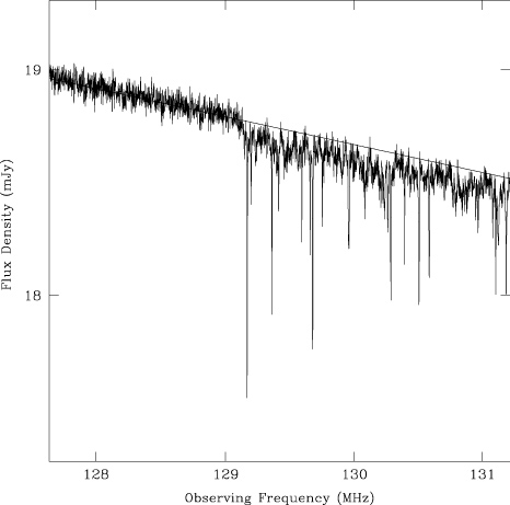
Figure 19. Simulated spectrum from 128 to 131 MHz of a source with brightness S(120 MHz) = 20 mJy at z = 10 using a model spectrum based on that of Cygnus A and assuming H ɪ 21 cm absorption by the IGM. Thermal noise has been added using the specifications of the SKA and assuming 10 days integration with 1 kHz wide spectral channels. The solid line is the model spectrum without noise or absorption. Reproduced with permission from [185]. Copyright 2002 American Astronomical Society.
Download figure:
Standard imageSince the evolution of the optical depth depends on the mean neutral fraction and the spin temperature, we can understand the evolution of the 21 cm forest based on figure 4. At early times, the IGM is fully neutral and the evolution is dictated by the spin temperature. TS tracks the gas kinetic temperature and rises from tens of Kelvin to thousands of Kelvin by the end of reionization, causing
 to fall by several orders of magnitude due to heating alone. Then, as reionization takes place and the neutral fraction drops from xH = 1 to the xH ∼ 10−4 seen in the Lyα forest, the optical depth drops even further. Tracing the evolution of the mean optical depth would provide a useful constraint on the thermal evolution of the IGM and give a clear indication of the end of reionization. Figure 20 shows the evolution of
in a model where TS = TK showing the very significant evolution in the optical depth with redshift.
to fall by several orders of magnitude due to heating alone. Then, as reionization takes place and the neutral fraction drops from xH = 1 to the xH ∼ 10−4 seen in the Lyα forest, the optical depth drops even further. Tracing the evolution of the mean optical depth would provide a useful constraint on the thermal evolution of the IGM and give a clear indication of the end of reionization. Figure 20 shows the evolution of
in a model where TS = TK showing the very significant evolution in the optical depth with redshift.

Figure 20. Mean 21 cm optical depth as a function of redshift, for varying fX values: from top to bottom, fX = 0 (no x-ray heating), 0.01, 0.1, 1 (thick black line), 10 and 100. Also included are lines of Smin (dashed purple lines) as defined in (65). These lines indicate, for each value of τ on the left-hand axis, the minimum observed flux density of a source that would allow a detection at a signal-to-noise ratio of five of the flux decrement due to absorption, assuming an array with effective area Aeff = 106 m2, frequency resolution Δνch = 1 kHz, system temperature Tsys = 100 K(ν/200 MHz)−2.8 and integration time tint = 1 week. When the mean optical depth lines (solid) cross above the Smin lines (dashed), the flux decrement is detectable at the corresponding redshift. Reproduced with permission from [187].
Download figure:
Standard imageDetecting the mean decrement in the 21 cm forest may be challenging since it is relatively weak and requires detailed fitting of the unabsorbed continuum level. A potentially more robust method is to exploit the statistics of individual features. As reionization occurs, the appearance of ionized bubbles will show up in the forest as an increasing number of windows of near total transparency. If these lines could be resolved, the distribution of equivalent widths would give a measure of the process of reionization [185, 186, 188].
It is possible that the forest does not have to be fully resolved and could be analysed statistically instead. For example, the appearance of ionized regions will lead to a change in the variance of the signal in different frequency bins. This has been shown to be an effective discriminant of the end of reionization [187] and has the advantage of not requiring narrow features to be resolved in frequency.
The signal from the diffuse IGM leads to a relatively low optical depth, as seen in (63). The signal from minihalos can be considerably stronger [122, 186, 189]. These are structures that have collapsed and virialized, but because of their low mass do not reach the temperature of 104 K required for atomic hydrogen cooling. Their high density contrast and relatively low temperature can lead to optical depths as high as τ ∼ 0.1 within a frequency width of Δν ∼ 2 kHz [190]. The mean overdensity required to give an optical depth τ is given by

The number density of minihalos is sensitive to the thermal properties of the IGM, which if heated may raise the Jeans mass sufficiently to prevent the collapse of the least massive minihalos that dominate the signal in the forest. Detailed descriptions of line profiles and their statistics have been considered based upon analytic models of the density distribution around halos [186, 189, 191, 192] and in high resolution simulations [125]. Even a single line of sight showing such structures could be used to provide information on early halo formation.
Unfortunately, the sensitivity required to detect the 21 cm forest is challenging. We can consider the thermal noise required to directly detect the flux decrement arising from the mean absorption. Using the relationship Sν = 2kBTa/Ae to relate the antennae temperature to the flux sensitivity for a single polarization and the radiometer equation gives the minimum source brightness for the decrement to be visible:

where we have assumed that both polarization states are measured. The value of Aeff/Tsys used is appropriate for SKA giving a sense of the challenge in detecting the forest. The system temperature is typically set by the sky temperature and is determined by galactic foregrounds.
The major uncertainty in the utility of the 21 cm forest is the existence of radio-loud sources at high redshifts. The most promising set of sources are radio-loud quasars. We are currently ignorant of the number density of radio-loud quasars at high redshifts. Quasars have currently been observed to redshifts as high as z = 7.1 [193], but their number density drops rapidly at redshifts z ≳ 3 [194]. Furthermore, the radio-loud fraction of quasars is poorly understood and may evolve at higher redshifts [195]. Models calibrated to the number of counts at low redshifts lead to predictions of ∼2000 sources across the sky with S > 6 Jy at 8 < z < 12 [196]. Many of these sources would show up in existing radio surveys, but it is currently impossible to distinguish these high-z radio-bright quasars from low-z radio galaxies. Future large area surveys with near-infrared photometry, such as EUCLID or WFIRST could enable the identification of these high-z quasars providing targets for the SKA [197]. Gamma-ray bursts (GRBs) and hypernovae may provide alternative high-z sources [198–200], but are believed to have a lower maximum brightness at the low frequencies of interest because of synchrotron self-absorption. GRBs do however have the virtue of already having been observed in the desired redshift range.
This rapid decline in radio-bright quasars is unfortunate since the signal is most strong early on before ionization and heating have begun significantly. In any case, it seems likely that only a few sight lines to radio-bright objects will become available for 21 cm forest observations. Since these observations are affected by totally different systematics than 21 cm tomography, they could be very important for identifying the properties of the IGM in the early Universe.
7. Conclusions and outlook
Cosmology in the 21st century is engaged in the process of pushing the boundaries of sensitivity and completeness of our understanding of the Universe. Observations of the redshifted 21 cm line offer a new window into the properties of the Universe at redshifts z = 1–150 filling in a crucial gap in observations of the period where the first structures and stars had formed. The 21 cm signal depends upon physics on different scales from the atomic physics of hydrogen, through the astrophysics of star formation, to the physics of cosmological structures. Through this dependence the 21 cm signal has enormous potential to improve our understanding of the Universe. Over the next decade, radio experiments will begin the process of exploiting 21 cm observations and will reveal how much of this potential can be realized.
In this review, we have explored four key ways in which 21 cm observations might be exploited to learn about cosmology and astrophysics. Low angular resolution observations with small numbers of radio dipoles can measure the sky-averaged 'global' 21 cm signal providing information about key milestones in the history of the Universe. Understanding these moments when the first radiation backgrounds illuminated intergalactic space will place constraints on the properties of the first galaxies and limit the contribution of more exotic physics. Experiments involving just a handful of people, such as EDGES and CoRE, have taken the first steps along this path. There is currently a growing effort to using different radio dipole designs and attempting to combine the benefits of interferometers with individual absolutely calibrated dipoles. There is a significant challenge in separating a relatively smooth 21 cm signal from smooth galactic foregrounds and much hard work ahead before these experiments yield robust results.
More ambitiously, collections of thousands of dipoles, digitally combined into radio interferometers will have the raw sensitivity to measure fluctuations in the 21 cm signal, providing detailed information about how the Universe was heated and ionized. The first generation of such instruments—LOFAR, MWA, PAPER and 21CMA—have or will soon be completed and data are starting to become available. These first instruments will peer through a hazy window of low sensitivity, but should determine when the EoR took place. Looking further ahead, the SKA will see this period clearly mapping the ionized structures and providing information about heating and coupling of the IGM during the formation of the first galaxies. The combination of 21 cm observations with observations of the CMB and with surveys of high redshift galaxies and information from the Lyman alpha forest should enable the reionization history and details of reionization to be inferred [201, 202].
21 cm observations also have the potential to constrain fundamental cosmology and represent a path to a new level of precision cosmology. Exploiting 21 cm observations for fundamental cosmology will be a challenging task and it is unclear how much can realistically be hoped for. During the EoR astrophysics mixes with cosmology in the 21 cm fluctuations and until the performance of instruments is better understood it is not clear whether these two can be separated. In the further future, 21 cm observations of the cosmic Dark Ages provide a long term hope that most of the volume of the Universe could one day be mapped and used for cosmology.
Applying similar techniques at lower redshifts allows for IM of the neutral hydrogen in galaxies, providing an alternative to traditional redshift surveys of galaxies in the optical–infrared bands. In contrast to the traditional approach, only the cumulative line emission from many galaxies over large volumes is being mapped, and galaxies are not being resolved individually. This IM technique could help shed light on the properties of dark energy through the use of BAOs as a standard ruler to measure the expansion of the Universe. Further, IM in other molecular and atomic lines can complement 21 cm tomography allowing a complete picture of the formation of stars and metals to be developed.
Finally, observations of individual radio-bright sources, such as quasars, might allow observations of the 21 cm forest. This provides another window into the properties of the IGM at the end of reionization that depends on very different systematics than 21 cm tomography. The 21 cm forest would allow the small-scale properties of the IGM to be studied in great detail and so constrain the properties of dark matter. This is a powerful technique and the main uncertainty is the abundance of target sources. Large area near-infrared surveys should begin to answer this question soon, as more high redshift quasars are found and followed up to determine the radio-loud fraction. Just a handful of sufficiently bright radio sources at z ≳ 7 would make this a very valuable probe of reionization and the IGM.
21 cm cosmology is a new field with much yet to be discovered, but it is one with great potential for the future. Much of this potential stems from breakthroughs in computing power which make 'digital radio astronomy' feasible and allow for extremely large radio interferometers. It is to be hoped that in the decades to come 21 cm observations will transform our understanding of the cosmic dawn and the EoR pushing farther our detailed understanding of the cosmos.
Acknowledgments
AL acknowledges funding from NSF grant AST-0907890 and NASA grants NNX08AL43G and NNA09DB30A. We thank Adem Lidz for producing figure 18 and for detailed comments on an early draft.
Footnotes
- 1
This is similar to the suggestion of using the 21 cm map as a template to detect the deuterium hyperfine line [13].