DO PERIODICITIES IN EXTINCTION—WITH POSSIBLE ASTRONOMICAL CONNECTIONS—SURVIVE A REVISION OF THE GEOLOGICAL TIMESCALE?

In this paper, we will present the results of power spectral computation of extinction rates derived from the Sepkoski (2002) compendium (hereafter SEP) of genus origination, extinction, and total biodiversity over the last ∼500 Myr.

Motivated by the finding of Raup & Sepkoski (1984) of a 26 Myr extinction periodicity in marine families, Melott & Bambach (2010) undertook to examine this question using new data on genera with revised timescales. We analyzed both the Sepkoski genus data and the Paleobiology Database (PBDB) for periodicity of extinction using the 2004 timescale and found that both display a periodicity in extinction at approximately 27 Myr that extends over 470 Myr. The original finding extended back 250 Myr. The expansion from 26 Myr to 27 Myr is not unexpected, as the geological timescale had expanded by about 3%. We also noted that 10 of the 19 mass extinctions as defined by Bambach (2006) lie within ±3 Myr of the maxima in the spacing of the 27 Myr periodicity when the timing is extended over the entire Phanerozoic (the last 542 million years), which differs from a random distribution at the p = 0.01 level.

The only change here in the extinction data from Melott & Bambach (2010) is the alteration of the dates of interval boundaries to coincide with the new 2012 geological timescale. Extinction during an interval is assigned to the end of the interval, because not only are major mass extinctions interval-bounding events, but even ordinary extinctions appear to be primarily pulsed and concentrated at the end of intervals—although of course there is some constant background level of extinction (Foote 2005).

In this study examining extinction data using the revised 2012 timescale, we also identify periods of marked extinction intensity based on a technique developed in a study of mass extinctions (Bambach 2006). It was necessary to re-evaluate what intervals were characterized as of marked extinction intensity rather than just using previously designated mass extinction events because adjustments in the timescale altered interval lengths and thus one of the ways in which rate of extinction is expressed. Now we find 19 such intervals occur over the last 470 million years (with another six occurring in the earlier Cambrian period, for which time correlations are uncertain and evolutionary dynamics are different, and so are not considered here). Ten of the 19 (coincidentally the same numbers as reported in Melott & Bambach 2010 for the 540 million years including the Cambrian period, but the revised data used in this new study are confined only to the last 470 Myr when time correlation of interval boundaries are secure) lie within ±3 Myr of the maxima in the spacing of the 27 Myr periodicity, which differs from a random distribution at the p = 0.01 level. Although this statistical test uses different criteria, it is dependent on the SEP data, so it is not a fully independent test.

However, the statistical test based on the PBDB data is fully independent and constitutes a specific check of the hypothesis. One might argue that it is not independent because the data were taken on the same planet. However, the data are predominantly different observations of fossil occurrences and were handled very differently, with substantial corrections applied, which were not applied to the SEP data.

Computations shown here, as in Melott & Bambach (2010) were performed on AutoSignal 1.7, sometimes supplemented by our own software. We have used both Lomb periodograms of unmodified data and fast Fourier transform of data interpolated (linearly at 1 Myr intervals between adjacent data points). Extensive discussion of the interpolation procedure is found in Melott & Bambach (2011a). Judicious interpolation and ordinary fast Fourier transform methods give essentially equivalent results for these data to Lomb–Scargle methods over the range of interesting frequencies. As the interpolation required for FFT constitutes an effective small amount of smoothing, the amplitude of the peak at 27 Myr is slightly reduced in the FFT computation, but even so it reaches a confidence level of p ∼ 0.02 assigned by AutoSignal (Figure 1(a)). This amplitude is higher than found in Melott & Bambach (2010) for the SEP data. Therefore, the improvement in the timescale has strengthened the signal. Intuitively, it would seem that a signal which improves with better calibration is a positive sign of its reality.

Zoom In Zoom Out Reset image size

In Figure 1(b), we show a Lomb periodogram (Scargle 1982, 1989) of the PBDB data extinction rates as given by Alroy (2008). Interpolation is not used here for the PBDB data, as its intervals are quite large compared with the 1 Myr steps used in interpolating required for FFT. The Lomb–Scargle procedure (also discussed and compared with FFT in Melott & Bambach 2011a) is essentially a method of constructing a Fourier series for data sampled at irregular intervals—a common occurrence in both paleontology and astronomy. The amplitude shown in Figure 1(b) is essentially the same as found for PBDB and the 2004 timescale used in Melott & Bambach (2010)—a natural consequence of the fact that the corrections in going from the 2004 to 2012 timescale are relatively smaller compared to the coarse time resolution of PBDB. So, a peak at the same frequency is present in these two independent data sets.

In work to be presented elsewhere (Melott & Bambach 2013), we show a more extensive analysis of both the SEP and PBDB data on extinction, as well as the relationship of the timing of intervals of marked extinction intensity to the phase of the periodicity, and examine the possible causal relationships. This note is restricted to the simple point that the periodicity has survived a rescaling of geological time, and with it, our objections (Melott & Bambach 2010) to the Nemesis hypothesis as a causal mechanism. With the rescaling the periodicity in the SEP data has gone from 27.13 Myr to 27.21 Myr; in the PBDB data it has gone from 26.79 Myr to 26.93 Myr.

As this manuscript was being prepared, a paper appeared (Feng & Bailer-Jones 2013, hereafter FB-J) which discussed fits to galactic motion and simple periodicities as compared with "biodiversity" data. They argue that Bayesian statistical analysis does not give any support for either periodicity or coincidence with astronomical, particularly galactic, motion of the Earth. There appear to be a number of problems with this study. We will discuss only those related to the detection of simple periodicity, possibly with an underlying trend. Although some of our comments will apply also to the analysis of relationship to galactic motion, this is a side issue and not treated here. We have already published on how uncertainty and complexity in the galactic mass distribution and velocity field confound precise comparison with terrestrial characteristics (Overholt et al. 2009). We also comment on some issues related to the detection of the 62 Myr periodicity in marine biodiversity (Rohde & Muller 2005; Lieberman & Melott 2007; Melott & Bambach 2011a, 2011b, and references therein), which FB-J claim to re-examine.

Melott & Bambach (2010) cited here was not cited in the FB-J paper. FB-J cite a "Melott & Bambach (2010)," but their listed citation was actually published in 2011, and is 2011b here. The "Melott & Thomas (2009)" they cite was published in 2009. All of these were already published when their paper was submitted.

FB-J discuss the 62 Myr periodicity in marine biodiversity first uncovered by Rohde & Muller (2005). Biodiversity is a product of both origination and extinction. Biodiversity increases when origination exceeds extinction and decreases when extinction exceeds origination. The behavior of just one of these phenomena does not, alone determine biodiversity. Rohde & Muller (2005) and Melott & Bambach (2011a, 2011b) dealt with biodiversity data (the number of kinds of organisms present) when documenting the 62 Myr periodicity in marine biodiversity. However, in their entire paper FB-J only examine extinction rates and events and apparently did not deal with biodiversity (even though they used the term in implying their study showed no strong 62 Myr periodicity), whereas this periodicity in biodiversity has been shown to result from the coherent interaction of extinction and origination fluctuations, and neither origination or extinction alone produce a strong signal (Lieberman & Melott 2007; Melott & Bambach 2011b). FB-J incorrectly refer to the extinction data as "biodiversity."

In assessing the evidence for biodiversity fluctuations, FB-J ignore the substantial effect found by Melott & Bambach (2011b), wherein the effect of the 62 Myr biodiversity periodicity is found to be diluted in the last 150 Myr by the accumulation of long-lived genera, apparently resistant to the cycles. When long-lived genera are removed, the intensity remains strong up to the recent. This is not a severe impediment to the detection of extinction periodicity, but it would be if they were actually examining biodiversity, as claimed.

FB-J examine the fractional extinction rate inferred from the Sepkoski data as reported by Bambach (2006) and from the PBDB data as reported by Alroy (2008). They also examine the timing of mass extinctions as reported by Bambach (2006). All these sources of data are based on the 2004 geological timescale. In doing so, there is no indication in the text that they have converted to the 2012 geological timescale, as we have here. The results of our re-analysis of the extinction data using the revised timescale, as reported above, document that the 27 Myr periodicity has somewhat increased strength. As will be seen below, this signal is only significant when the actual timing of most extinction is assigned correctly.

FB-J importantly describe the hypothesis as, for example, "a periodic model". The Bayes factor (likelihood ratio; see, e.g., Wang 2010; D'Agostini 2003) is taken as an average computed over all possible phases and periods 10–100 Myr. The substantial past literature on this question does not ask whether "a periodic model" is the best description of the data. In fact, there are theorems, now at textbook level, which show that virtually any mathematical function may be represented as a sum of sinusoids. In these, one frequency will nearly always be dominant. Instead, it is relevant to ask how often random data might produce a dominant frequency comparable in amplitude to that found in the data.

It might be asked whether Bayesian, frequentist, or exploratory data analysis is appropriate to this problem. Bayesian and frequentist methods begin with a problem, go to the data, apply a model—then diverge from one another, either to analysis or to the application of a prior distribution. In exploratory data analysis (Tukey 1977), the next step from data is the analysis of the data to suggest a model—which is then subjected to hypothesis testing. The guiding principle is the statement by Tukey (1962): "Far better an approximate answer to the right question, which is often vague, than an exact answer to the wrong question, which can always be made precise." Exploratory work by Raup & Sepkoski (1984) suggested a periodicity in extinction at 26 Myr on the older timescale, that by Rohde & Muller (2005) a periodicity in biodiversity at 62 Myr. Further work should focus on testing these hypotheses.

Rohde & Muller (2005) did a number of Monte Carlo tests in which they randomized the data. They showed that the probability of any periodicity, that is, at any period, arising at the strength equal to or larger than the one they detected, is 0.01 (or less, depending on details of how the data are reordered). This significance level agrees with estimates made using AutoSignal (e.g., Melott & Bambach 2011a).

This is a crucial point. FB-J assert that random data may produce a strong periodicity, so finding some periodicity that fits is not significant. However, they do not ask how likely this is given the data and given the strength of the spectral peak, nor do they mention the tests by Rohde & Muller. Furthermore, they assert that they are testing the viability of periodic models by averaging over all such models. This of course dilutes any benefit of hitting the "correct" model—which is actually rather well specified.

FB-J have assigned both mass extinction events and "continuous" extinction rates to the middle of the interval in question. However, as noted in Foote (2005) there is considerable evidence that most extinctions are pulsed and concentrated at the end of intervals and it is certainly the case for most larger extinction events, because these events are used to set interval boundaries. Therefore, it is a better approximation to assign extinctions to the end of intervals than to the midpoints. These intervals range from 7 to 18 Myr for PBDB and 2 to 9 Myr for the SEP data. For most extinction data, the FB-J choice results in a systematic and varying error of a shift to earlier dates, which will degrade the signal. The degradation will be greater for the 27 Myr signal than for the 62 Myr signal, because the errors constitute a greater phase angle. The effect on obscuring the 27 Myr periodicity of extinction when an inappropriate location of extinction within intervals is used will be shown with an example below.

FB-J assign an uncertainty to the extinction data derived from the length of the interval to which they are assigned. This is almost certainly (see Section 3.6) an overestimate of the true uncertainty in date assignments, since the uncertainty in geological date assignments varies with their date, but is now typically less than ±1 Myr. For example, the end-Permian extinction, the most severe known, is now known to have occurred within 200,000 yr of a volcanic ash dated at 252.28 ± 0.08 million years ago (Shen et al. 2011) and the end-Cretaceous extinction, famous for the extinction of the dinosaurs, occurred within 30,000 yr of 66.043 ± 0.05 million years ago (Renne et al. 2013). About 2/3 of all the interval boundaries we consider have 95% errors less than 1 Myr, and only four of them have errors exceeding 2 Myr. None exceed 3.2 Myr. (We must allow for the possibility that systematic error is greater than this random error—but even systematic errors, estimated as the difference between 2004 and 2012 timescale dates, exceed 3 Myr only about 30% of the time.) FB-J consider standard deviations in the extinction timing which are various multiples of the standard deviation of the interval. Consequently, nearly all the FB-J assignments of extinctions are outside the 95% confidence interval for the timing, and more than 2/3 exceed the estimated systematic error. When the assumed uncertainty in the extinction timing is a small multiple, their assignment to the interval midpoint will result in a "miss" for the 27 Myr periodicity. When this is a large multiple, any "hit" will have lowered significance in their Bayesian procedure due to large uncertainty in the data.

FB-J compare the evidence for various models, averaging over all sets of parameters. They correctly note that the Bambach (2006) list of extinction events is not independent of the SEP data. However, they ignore the fact that the SEP and PBDB data were compiled separately and are independent data. Thus, one can formulate the hypothesis in a new way: is the biodiversity period found in the SEP data also found in the PBDB data? This question was already answered affirmatively in Melott (2008) and Melott & Bambach (2011a); in the latter the same periodicity was also found in a third data set. The same is true for the 27 Myr periodicity of extinction. It occurs in both SEP and PBDB data, as reported in Melott & Bambach (2010) for the 2004 version of the timescale and in this paper. Two additional statistical tests are possible, as shown in those papers, in which the question is formulated as finding agreement of a period with that already found in independent data. FB-J chose not to do such tests.

As related to the question of testing the general question of periodicity versus specific sets of parameters, FB-J also ignore the finding of periodicities coincident with biodiversity fluctuations within the errors in period and phase in the emplacement of sediments (Melott & Bambach 2011b; Meyers & Peters 2011) and strontium isotope ratios in seawater (Melott et al. 2012). Of course, as a formally constituted statistical question, these are not relevant: FB-J were claiming to test for biodiversity signals. But the practical scientific issue is that these variables are known to be related to biodiversity and extinction, as discussed in these references.

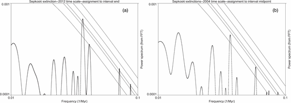
For all these reasons, we do not accept the conclusions of FB-J. As an example of the effects of some of their errors, we show in Figure 2(b) the power spectrum of the SEP data extinction rates if we assign our data to the mid-points of the intervals and use the 2004 geological timescale, paralleling the choice made by FB-J. This can be compared directly with Figure 2(a), a power spectrum of SEP data using the 2012 geological timescale and assigning the data to the interval end boundaries, where we know they are concentrated. As can be seen, although the 27 Myr peak is still visible in Figure 2(b), its amplitude is degraded. Treating the data as FB-J treat it reduces the significance of the signal that is unambiguously present when the data are treated more correctly. The significance of the spectral peak which has p ∼ 0.02 in Figure 2(a) is reduced to p ∼ 0.2 in Figure 2(b).

Zoom In Zoom Out Reset image size