


ABSTRACT
We investigate the origin, configuration, and evolution of moving magnetic features (MMFs) in the moat and penumbra regions of NOAA AR 10930 using Hinode/SOT filtergrams and magnetograms. We differentiate MMFs into four types in terms of the location of first appearance and the source of initial flux. The main results are summed up as follows: (1) 50% of the MMFs are produced from or within the penumbra, while 50% are produced within the moat. The MMFs formed in the penumbra normally move outward along radial directions. The MMFs formed in the moat have more dispersed directions of motion. The average speed of most MMFs decreases radially. (2) About 63% of moat fluxes are input by flux emergences. Newly emerged MMFs are normally smaller in size. In their rise phase, they gain flux by adding newly emerging flux or merging other elements, and in the decline phase they lose flux by flux cancellation or fragmentation. The MMFs that are fragments separated from penumbra or other magnetic elements usually have larger flux and longer lifetime. They start their decay process once they are formed. Frequent merging and flux cancellation between MMFs are the dominant factors in MMFs' evolution. (3) Cancellations between opposite-polarity magnetic elements are responsible for most of the low chromospheric bright points. Bipole emergence and MMFs' severance from the penumbra also produce bright points. Elongated or horn-shaped micro-filaments may appear during the separation or cancellation process between magnetic elements.
Export citation and abstract BibTeX RIS
1. INTRODUCTION
High-resolution observations of small-scale magnetic features moving around sunspots in the photospheric and chromospheric layers contribute to a better knowledge of sunspot structure, and to the understanding of the transport of magnetic energy and mass throughout the chromosphere.
In many well-developed sunspots, a mean outflow is observed in both the penumbra and the surrounding moat region. In the penumbra, the magnetic field is strong and inclined, while in the moat it is weak. On magnetogram time series, moving magnetic features (MMFs) are observed to originate from the outer penumbra, become isolated magnetic elements, move radially outward into the moat regions, and eventually disappear among the network fields. A series of achievements on MMFs (Harvey & Harvey 1973; Vrabec 1974; Brickhouse & Labonte 1988; Lee 1992; Zhang et al. 1992, 2003; Shine & Title 2001; Yurchyshyn et al. 2001; Bernasconi et al. 2002; Hagenaar & Shine 2005; Sainz Dalda & Martínez Pillet 2005; Li et al. 2006, 2009, 2010; Ravindra 2006; Ryutova & Hagenaar 2007; Lim et al. 2012; Criscuoli et al. 2012; Sainz Dalda et al. 2012) are summarized as follows.
- 1.Most of these "steady flow of bright points" (Sheeley 1969) move at about 0.3–1.0 km s−1 along paths that are almost radially outward from the penumbra and form magnetic flux outflow.
- 2.MMFs tend to originate from certain azimuths around parent sunspots and follow particular paths. MMFs may first appear at 0''–10'' beyond the outer edge of the parent sunspot. Many of them have precursors that originate inside the penumbra.
- 3.MMFs exhibit a range of lifetimes (0.2–8 hr), radii (0
 5–2''), net fluxes (1–25× 1018 Mx), and bipole separations. They may also appear as bright features in G-band and Ca ii H images.
 - 4.Previous researches have categorized MMFs according to their parity (unipolar or bipolar), polarity (same or opposite to the parent sunspot), direction of motion (outward or inward), and dipole orientation (whether the inner/outer footpoint has the same polarity as the sunspot).
Complex interaction of turbulent convection, radiation, and magnetic field makes sunspots hard to model. The monolithic model (Cowling 1957) regards the sunspot as a magnetostatic and tight bundle of magnetic field lines. In the cluster model (Parker 1979a, 1979b), the bundles of magnetic flux tubes are loosely confined by subsurface converging downflows in the surrounding plasma.
The first model for MMFs proposed by Harvey & Harvey (1973) suggests that loose flux tubes, twisted by the interaction of the magnetic field with the supergranulation or granulation, are separated from the main body of the sunspot and further swept to the network by the supergranulation's velocity field. Wilson (1986) explained the outward moving of MMFs with an oscillatory velocity field that generates the new flux loops near the sunspot's limb. Spruit et al. (1987) suggested that MMFs are small pieces of large U-loops which rise to the surface from the convection zone. Thomas et al. (2002) explained MMFs as the submergence of penumbral magnetic flux by convective pumping.
Multi-wavelength observations (Zhang et al. 1992; Penn & Kuhn 1995; Zuccarello et al. 2009) have been performed in Hα and Ca ii H filtergrams. MMFs are almost invisible in Hα images, indicating that they are low-lying features. Zhang et al. (1998) analyzed the relationship between the fine structures of granulation and magnetic fields using a time series of Fe i λ5250.2 photospheric filtergrams and corresponding magnetograms in a quiet region. They found that, although most bright filigree features in photospheric filtergrams are related to corresponding magnetic features, they are generally not co-spatial. It is also found that some bright features and their corresponding photospheric magnetic fields show fast changes within several minutes.
Modern high-resolution observational efforts and techniques, especially space-based observatories, provide more details of MMFs than ever before. Kubo et al. (2007) studied isolated and non-isolated MMFs using coordinated Dunn Solar Telescope and Solar and Heliospheric Observatory (SOHO) observations. The magnetograms obtained by the Hinode observatory provide an opportunity to study the MMFs' motion in and out of sunspot penumbral fibrils (Ravindra 2006) and small-scale reconnection events (Guglielmino et al. 2010; Murray et al. 2012; Su et al. 2012).
However, the behavior and fundamental structure of MMFs are still not understood completely. It is still not clear how much their interactions with the upper and lower chromosphere contribute to the energy transportation through the chromosphere and the heating of the solar corona. A large-sample study of the details about their formation, evolution, fragmentation, merging, and disappearance is yet to be performed.
We devote the next two sections to introducing the data and the data processing. The results, summary, and discussions are presented in the later sections.
2. OBSERVATION
Hinode is a joint mission between the space agencies of Japan, United States, Europe, and United Kingdom (Suematsu et al. 2008). The Solar Optical Telescope (SOT), a diffraction-limited Gregorian telescope with a 0.5 m aperture, is one of the three instruments carried by the Hinode spacecraft. The SOT's instrument package, provided by NASA/LMSAL and referred to as the Focal Plane Package, contains the sub-systems which record the data used in this research: the Broadband Filter Imager (BFI), the Narrowband Filter Imager (NFI), and the Spectropolarimeter (SP). The BFI produces photometric images with broad spectral resolution in six bands to observe both photospheric and chromospheric structures under quiet and active solar conditions. The NFI's filter has selectable bandpasses in six key solar spectral regions which span the photosphere to the lower chromosphere for analysis of dynamical behavior of magnetic and velocity fields. It produces large field-of-view longitudinal flux density magnetograms with moderate polarimetric accuracy (4 × 10⁻³), also known as Stokes V/I magnetograms. Images from the NFI contain blemishes caused by air bubbles inside the tunable filter, which degrade or obscure the image over part of the field of view. SOT/SP records the photospheric vector magnetic fields of both quiet and active regions with the highest possible precision (10−3 or better). It uses Fe i λ6301.5 and Fe i λ6302.5 lines, both commonly used for photospheric magnetograms because of their Zeeman sensitivity.
Active region NOAA 10930 was a sizeable active region located in the southern hemisphere near the equator, spanning about 90'' east–west and about 100'' north–south. It consisted of a single large leading sunspot of negative polarity, two small sunspots of positive polarity, and several pores, as shown in Figures 1 and 2. AR 10930 first appeared on 2006 December 5 as a β region. Once it appeared, it showed intense activity. From December 6 to 8, it produced 3 X-class, 9 M-class, and 42 C-class events. The magnetic configuration changed from β to βγδ. During December 9–10, it became quiet with no major events. From December 11, it started producing events again, and its activities remained intensive until it rotated beyond the solar limb on December 18.
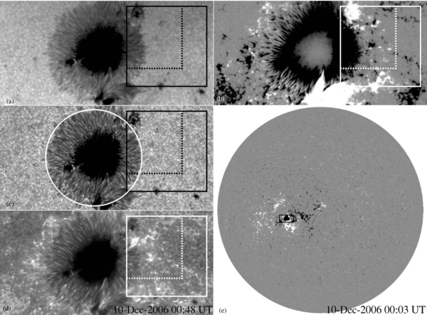
Figure 1. (a–d) Images of NOAA AR 10930 taken from the Hinode BFI and NFI time sequences acquired on 2006 December 10. They are (a) Fe i filtergram, (b) Stokes V/I magnetograms with white (black) showing positive (negative) polarity, (c) G-band filtergram, and (d) Ca ii H filtergram. The field of view is 127'' × 62''. The solid-line squares outline our region of interest, and the dashed-line rectangular area is used in Figure 3 for demonstration purposes. The circle in panel (c) is the least-squares fit to the penumbra outer boundary. (e) A full-disk magnetogram taken by SOHO/MDI on 2006 December 10. The observed active region was located near the disk center (S04E12). The rectangle outlines the field of view of images (a)–(d).
Download figure:
Standard image High-resolution image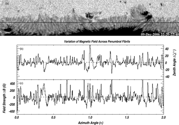
Figure 2. (a) Context image showing the penumbral fibrilla structure of AR 10930's major sunspot. The image is the Mercator projection of an annular region around the sunspot, extracted from a continuum intensity map taken by Hinode/SOT/SP. Many penumbra fibrils do not extend in the exact radial direction, but tend to group at certain azimuths. The horizontal dark line represents an ellipse concentric to the penumbral boundary. The size of this ellipse is 20% smaller than the sunspot. The ladder plot below is based on quantities measured along this ellipse. (b) The variation of magnetic field's zenith angle ζ across the penumbral fibrils. The abscissa is the polar angle; the ordinate is the small-scale variations of ζ, measured from an SOT/SP field inclination map. (c) The small-scale variations of the magnetic field strength B across the penumbral fibrils, measured from an SP field strength map.
Download figure:
Standard image High-resolution imageEighteen hour time sequences of Fe i filtergrams, magnetograms, G-band, and Ca ii H images of AR 10930 were obtained during the period of December 9 20:00–10 13:59 UT with the SOT. There were no major events during the observation period. The data were taken at a rate of 30 frames per hour. The G-band λ4305 and Ca ii H λ3968.5 filtergrams were taken by BFI with a spatial resolution of 0106 pixel−1 and a cadence of 120 s over a 218'' × 109'' field of view. The Fe i λ6302.5 filtergrams and λ6302.5–0.12 Stokes V/I longitudinal magnetograms were taken by NFI with a spatial resolution of 016 pixel−1 and a cadence of 120 s in a full-CCD frame field of view of 328'' × 164''. The NFI sequences are consecutive, but the BFI sequences have three 1 hr gaps. Figure 1 shows four images taken by NFI and BFI of AR 10930 on 2006 December 10. The region of interest that we selected is located to the west of the major sunspot, as outlined by a box with solid lines. In this 48'' × 48'' rectangular region, there was a constant outflow of MMFs; also included are the intensive interactions between the major and two minor sunspots. The imaging was not seriously affected by the projection effect or the blurring bubble in the SOT instrument. The sub-area outlined by dashed lines is used in this paper to demonstrate our image processing methods.
We also use the magnetograms taken by the SOT/SP instrument. Two SP observations were acquired in the "Fast Map Mode" during 22:00–23:03 UT on December 9, and 01:00–02:05 UT on December 10, with 0295 and 0297 step sizes of spectrograph slit scanning and 0317 and 0320 pixel scales in the y-direction, respectively. Another two SP observations were scanned later (times of the first slit position: 10:55 and 12:26 UT on December 10) in the "Normal Map Mode" with 0149 spectrograph slits and an 0160 step size. The SOT/SP level-2 data are outputs from inversions using the HAO MERLIN inversion code.1
3. METHOD
3.1. Preprocessing
We made animations of the time series of Stokes V/I magnetograms, Fe i, G-band, and Ca ii H filtergrams to investigate the motion of MMFs around the sunspots' penumbrae. MMFs' configurations and associated bright points are studied by comparing the magnetograms and their corresponding filtergrams. Bad images in the time series were removed and the final data set consists of 533 NFI frames and 470 BFI frames. The active region was first tracked in each data set by adjusting the heliographic coordinates, and then co-aligned using a two-dimensional Fourier transform cross-correlation program. The alignment of NFI images with the BFI images was achieved as follows: the NFI magnetograms and filtergrams were first interpolated into the same spatial resolution as that of BFI, and then were co-aligned and registered with the BFI G-band images.
3.2. Edge Enhancement
We intend to observe the filigrees, the granulations, and MMFs' precursors. But these features are hard to identify and follow with naked eye: the precursors are buried among strong magnetic background of the penumbra fibrils; the filigrees and the granulations are nebulous and change rapidly.
In order to highlight these features of interest, a spatial domain edge detection algorithm is applied to the time sequences to sharpen the fine details of the images and reduce noise. The results of Prewitt, Roberts, and Canny (Canny 1986) edge detection operators are added to the original image to enhance the contrast of the edges. Let I be the source image, then the filtered image can be denoted as
where  and
and  (
( and
and  ) are the horizontal and vertical results of Prewitt (Roberts) kernels, respectively, convoluted with the original data array, and
  is the arithmetic mean of the source image I. The row and column masks of the Prewitt (Roberts) operator are 3 × 3 (2 × 2) matrices. The Canny operator first performs noise reduction by Gaussian convolution, computes the gradient vectors, and then, through a process known as non-maximal suppression, traces intensity discontinuities with thin lines in the output image
  . Parameters a1, a2, and a3 are set manually.
The effects of this image processing technique are shown in Figure 3. In the original Fe i and G-band filtergrams (Figures 3(a) and (b)), the penumbra fibrils and the moat granulations are blurry. But after edge enhancement, their boundaries become clearer and easier to identify. Similarly, the filigrees and dark features also have a much higher contrast with the background. In the original magnetograms (Figure 3(c)), due to the strong magnetic strength of the penumbra, it is difficult to isolate any feature inside the sunspot. In the enhanced image, the penumbra fibrils are clearly visible.
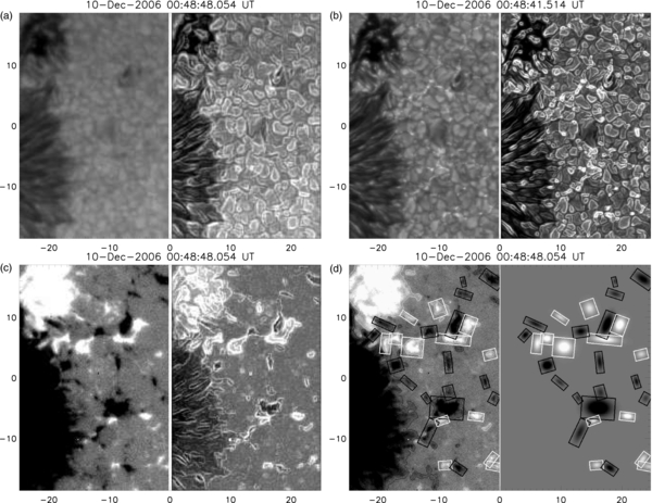
Figure 3. (a–c) Demonstrations of the edge enhancement technique (Section 3.2) applied in this research. In each panel of (a) Fe i λ6302.5 filtergram, (b) G-band filtergram, and (c) Stokes V/I magnetogram, the image on the left is extracted from the original time sequences, and the image on the right has been processed with our edge enhancement procedure. In these sharpened images, features in the penumbra and moat are much easier to distinguish. (d) Demonstrations of the measurement of MMFs based on two-dimensional Gaussian surface (Section 3.3). Left: sample magnetogram frame with contours overlaid. The identified MMFs are labeled with boxes. The flux density saturates at ±150 G. Right: the best-fitting Gaussian bulbs of the identified MMFs. The color, rotation, length, and width of the boxes represent the polarity, rotation, x' and y' spreads of the Gaussian bulbs. The field of view of these images is outlined by dashed lines in Figure 1.
Download figure:
Standard image High-resolution image3.3. Gaussian Measurement of MMFs
On magnetogram animations, magnetic elements of various sizes, shapes, strengths, velocities, and polarities are mixed and interacting in the inner moat region. This complexity makes the manual measurement of MMF's geometric and magnetic properties time-consuming and biased by observers. To avoid this problem, we developed a set of routines for the determination of the size, shape, magnetic flux, and center flux density of MMFs by measuring their best-fitting Gaussian surface.
The best-fitting Gaussian bulb of a magnetic object's flux density can be denoted as
where x' and y' are the coordinates in the intrinsic frame whose abscissa and ordinate coincide with the bulb's longer and shorter axes, Bn is the background magnetic strength, coefficient A is the amplitude of B, and  (
( ) is the x' (y') spread of the bulb. The measured profiles of MMFs' flux density (Section 4.1) suggest that the above two-dimensional Gaussian approximation is proper for MMFs.
The flux ϕ of the magnetic object measured by integrating the net flux density over an bulb-centered rectangle  is
is
where  and
and  are, respectively, the length and width of the rectangle which were selected to measure the magnetic object,
  (
( ) is the ratio between the rectangle's half-width
  (
( ) and the bulb's spread
  (
( ), and erf is the error function
  . The real flux of the magnetic object should be the entire volume of the bulb,

For each identified MMF on each frame, a Gaussian fit is performed on the local region, which yields A,  , and
, and  . These coefficients provide the magnetic flux using the formulation (5). The Gaussian fit procedure also measures the MMF's rotation, location, and background field strength Bn.
For those magnetic objects where the Gaussian fitting calculations do not converge, their real fluxes can be estimated by correcting the values measured through integration
where  and
and  are the Gaussian bulb's half-width at half-maximum (HWHM) whose determination does not require the Gaussian fit routine. Thus, the errors of the flux measurement caused by the uncertainties of the selection of the rectangles are compensated.
Figure 3(d) shows the result of this procedure on a magnetogram frame, in which the information of MMFs' magnetic and geometric properties is extracted from the complex magnetogram and is ready to be used for statistical study.
3.4. Estimating the MMF's Lifetime and Birth Rate
For each identified MMF, we record its appearance and disappearance. Since the observation of those MMFs with longer lifetimes is more likely to be interrupted by the ends of the time sequences than that of short-lived ones, selection of the samples is not objective. Thus, arithmetic calculations of characteristic values such as lifetime, population, and production rate would certainly be biased by the limited time duration of observation. We propose the following method to compensate for this bias. The method yields relatively good estimations on artificial data.
The frequency distribution of MMFs' lifetimes, F(T), can be estimated by

in which T is MMFs' lifetime, D is the duration of observation, and Fo(T) is the observed frequency of those MMFs whose entire lifetime is within the duration of observation. Thus, the estimated population of newly produced MMFs during the observation is

3.5. Composite Evolution Function
We calculate composite evolution functions to study the evolution of the magnetic flux, central flux density, and area of all the MMFs observed in the region of interest. These functions merge the individual characteristics of a set of MMFs, describe the most common pattern of their evolution, and inherit their average magnitude and lifetime. Here we take MMFs' magnetic flux as an example to present our formulation of the composites.
The whole MMF population is divided into ng × nτ subsets by their location and type. ng is the total number of observed active regions, and nτ is the number of nominal categories specifying the types of the MMFs. In our observation, ng = 1 and nτ = 4.
For each identified MMF, on each frame of the time sequence, its magnetic field is measured using methods described in Section 3.3. Its flux as a function of time is denoted by the symbol

where the MMF's type τ ∈ {α, β, γ, θ} (see Table 1), index number i ∈ {1, 2, ..., N(τ, s)}, the region of observation s ∈ {1, 2, ..., ng}, N(τ, s) is the subset population, and  is the MMF's lifetime. Thus,
  stands for the flux of type τ MMF numbered i in region s measured at moment t.
Table 1. Categorization of MMFs
| Initial Location | Source of Initial Flux | |
|---|---|---|
| Flux Emergence | Fragmentation | |
| Penumbral boundary | α | β |
| Moat | γ | θ |
Download table as: ASCIITypeset image
The composite evolution function of a subset,  , shows the most common pattern of flux evolution of type τ MMFs in region s.
where  is an MMF's weighted average flux on the n frames it appears
  .
.  and
and  are, respectively, the average flux (
 ) and average lifetime (
 ) of the subset.
The composite evolution function of all the observed type-τ MMFs is calculated from the ng subset composites,
where 〈ϕτ〉 and 〈Tτ〉 are, respectively, the average flux ( ) and average lifetime (
 ) of the ng subsets. Each MMF subset has equal weight on the overall composite.
4. RESULTS
Active region NOAA 10930 comprised a major sunspot of negative polarity and two tightly attached small sunspots with positive polarity in the northwest and south directions. Between the major and minor sunspots there were highly sheared penumbral fibrils. The interlaced fibril structure of the major sunspot's penumbra can be seen in a Mercator projection (Snyder 1987) of the penumbra and inner moat region (Figure 2(a)), and also in the variation of the amplitude and zenith angle of the penumbra's magnetic field (Figures 2(b) and (c)). Several small pores of both polarities emerged during our observation. The two minor sunspots, especially the one to the south, are well connected to the pores on the southwest side of the major sunspot by penumbral extension. We established least-squares fitting circles of sunspot limb (Figure 1(c)), and set up polar coordinates to determine the positions of MMFs, using contours of the penumbra's outer boundary on time-averaged G-band filtergrams.
Animations show that at all times there is a continuous expulsion, emergence, fragmentation, merging, and disappearance of magnetic features, especially at the contact region of the major and minor sunspots. On our region of interest, we have identified and traced 240 MMFs over the time series. Their origins and displacements are plotted in Figures 4(a) and (b). The MMFs are monopolar as well as bipolar in nature. Most of the bipolar MMFs are seen to originate at the penumbral fibrils. In the animation of intensity images, many MMFs are either invisible or have weak contrast, but some MMFs appear as bright dots or dark patches.
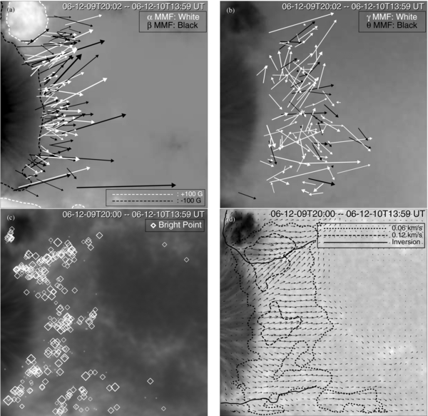
Figure 4. (a) The origins and displacements of the identified MMFs that originate from the penumbrae. Each arrow marks the initial and final locations of an MMF. The thickness represents the MMF's magnetic flux. Black arrows stand for β-MMFs that have the same polarities as their parent sunspots. The α-MMFs that have polarities opposite to the penumbra are marked with white arrows. The approximate peripheries of the sunspots are delineated with contours of ±100 G. (b) The displacements of the MMFs that originate in the moat. Black and white arrows represent moat MMFs that are produced by fragmentation (θ) and emergence (γ). (c) A demographic map of the Ca ii H bright points that appeared during our observation. The size and thickness of the diamonds are determined by the size and brightness of the bright points. (d) The arrows indicate the time-averaged horizontal velocity field constructed by local correlation tracking method using longitudinal magnetograms. The dashed contours circle regions that have high flow speed. The solid curve delineates the sheared polarity inversion lines between the major and minor sunspots. The background images for these panels are time-averaged (a) Stokes V/I magnetogram, (b) Fe i, (c) Ca ii H, and (d) G-band filtergrams.
Download figure:
Standard image High-resolution image4.1. Distribution of MMF's Magnetic Strength
The magnetic flux of the observed MMFs ranges from 0.3 × 10¹⁸ to 55 × 1018 Mx. Figure 5(a) shows a histogram of their fluxes. The smallest distinguishable magnetic elements have fluxes of about 0.05× 10¹⁸ Mx. At the right end of the distribution are a few large MMFs which developed into pores. This distribution can be fitted with a lognormal model:

The dashed line in Figure 5(a) is fitted with Equation (12), where a0 = 13.54 and a1 = −4.76. The number of small magnetic elements can be estimated by Equation (12). The median of this distribution model is 3.2 × 10¹⁸ Mx, i.e., in an exhaustive observation of MMFs, the population of MMFs with flux less than 3.2 × 10¹⁸ Mx should be approximately equal to the total number of those that have a flux greater than 3.2 × 10¹⁸ Mx. After similar calculations, it is found that the frequency distributions of MMFs' area, lifetime, and displacement are all similar to Figure 5(a) and therefore can be fitted by Equation (12). These suggest the existence of a large number of small short-lived MMFs.
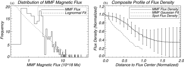
Figure 5. (a) The frequency distribution of the magnetic fluxes of the MMFs that we observed. The dashed line is the lognormal fit of the histogram. (b) The solid curve shows the profile of MMF's flux density along the radial direction. It is a composite of all the individual MMFs' profiles computed from longitudinal magnetograms. The abscissa is the normalized distance to the MMF's flux center. When the distance equals the MMF's HWHM, the normalized value is 1. The ordinate is the normalized value of flux density, and the error bars show the standard deviations. The dashed curve shows the result of Gaussian fit using Equation (13). The dash-dotted curve is the profile of the flux density of AR 10930's major sunspot.
Download figure:
Standard image High-resolution imageWe have investigated the two-dimensional distribution of flux density inside the MMFs on Stokes V/I line-of-sight magnetograms. For each MMF's appearance on each frame of a magnetogram, we locate its flux center, determine its HWHM ro, and measure its flux density profile B(r) as a function of distance to the flux center. On average, each MMF is measured on 72 frames. Then, these profiles are normalized to filter the amplitudes of each individual MMF's radius and flux density. The normalized profiles have been further combined into one single composite profile  , as plotted in Figure 5(b) (solid curve). The error bars show the standard deviations. The dashed curve shows Gaussian fit using the equation
where a0 = 0.6531, a1 = 0.6159, and a2 = 0.3342. The almost seamless fit of the Gaussian function could mean that the distribution of MMF's flux density is Gaussian along its radius. Figure 5(b) also compares the profile of MMF's flux density with that of sunspots. The dash-dotted curve is the flux density profile measured on the major sunspot of AR 10930.
4.2. Categorization
We categorize MMFs into two categories and four types according to the location of their first appearances and the source of their initial magnetic flux.
- Penumbral MMFs. They originate inside or immediately outside the outer penumbral boundary, separate from penumbra fibrils, and move outward. They are differentiated into two types by their polarities.
- α-MMF. Having the polarity opposite to the parent sunspot.
- β-MMF. Sharing the parent sunspot's polarity.
- Moat MMFs. They originate outside the penumbra outer boundary, and first appear among moat granulations, with no obvious connection with penumbra fibrils. They are also differentiated into two types according to whether they are attached to other MMFs when they first appear.
- γ-MMF. Emerge in the moat, with no obvious affiliation to other magnetic objects.
- θ-MMF. A fragment separated from a magnetic object in the moat.
As shown in Table 1, β- and θ-MMFs are products of fragmentation, and their initial fluxes come from their parent magnetic objects. α- and γ-MMFs are newly emerged magnetic objects.
MMFs can disappear by fragmenting into smaller magnetic elements, merging into other magnetic objects, or diminishing below the threshold of observation. However, the extinction of MMFs is not considered in this categorization.
4.3. MMFs Formed from Penumbra
Penumbral MMFs first appear inside or near the periphery of penumbra. Precursors of penumbral MMFs sometimes can be identified inside the penumbral boundary on edge-enhanced magnetograms (Figure 3(c)). Once they leave the penumbra, penumbral MMFs move outwardly along the radial direction into the moat (Figure 4(a)). β-MMFs are produced close to the penumbral boundary and carry a large amount of flux, while α-MMFs emerge farther from the penumbra, and are small in size and weak in flux (Table 2). This agrees with Li et al.'s (2009) observation.
Table 2. Basic Physics Quantities of the Four Types of MMFs
| Quantity | All | α | β | γ | θ |
|---|---|---|---|---|---|
| Share of total MMF population (%) | ⋅⋅⋅ | 25.8 | 23.8 | 39.6 | 10.8 |
| Share of total MMF flux (%) | ⋅⋅⋅ | 27.1 | 33.4 | 30.4 | 9.1 |
| Lifetime (hr) | 1.57 | 1.60 | 1.97 | 1.37 | 1.87 |
| Initial dist. to penumbra (arcsec) | 5.15 | 2.60 | 1.35 | 9.56 | 11.74 |
| Final dist. to penumbra (arcsec) | 10.55 | 8.05 | 6.51 | 12.89 | 15.31 |
| Displacement (arcsec) | 4.53 | 4.57 | 5.28 | 4.38 | 4.51 |
| Speed (km s−1) | 0.56 | 0.55 | 0.59 | 0.65 | 0.36 |
| Acceleration (m s−2) | −0.30 | −0.27 | −0.20 | −1.06 | −0.06 |
| Radius (arcsec) | 0.91 | 0.76 | 1.03 | 0.85 | 0.92 |
| Flux density (G) | 161 | 137 | 188 | 147 | 175 |
| Magnetic flux (1018 Mx) | 2.73 | 1.62 | 4.95 | 2.50 | 2.70 |
Notes. Rows 1 and 2: the shares of population and magnetic flux held by each category of MMFs. Rows 3–11: average values of the quantities measured in the four subsets of MMF samples.
Download table as: ASCIITypeset image
Figure 6 shows time series of magnetograms with two examples of penumbral MMFs. The top two rows (Figure 6(a)) show the motion of a positive polarity α-MMF, which emerged among magnetic negative penumbral fibrils. The bottom two rows (Figure 6(b)) are the serial images of a β-MMF which is a parcel of the penumbra that separated from the fibrils and moved outward.
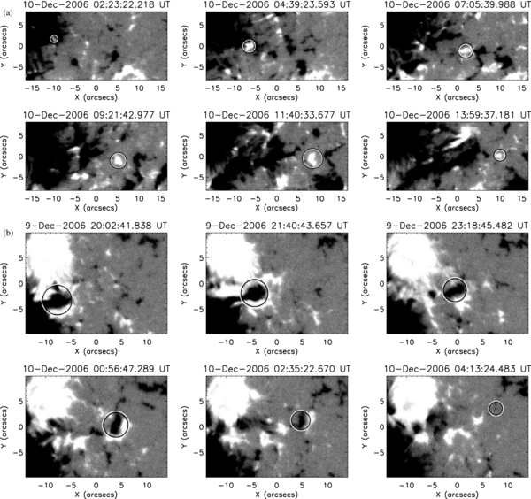
Figure 6. Sequences of magnetograms of two typical MMFs that formed from the penumbra. (a) An α-MMF's emergence and motion. The circles indicate the locations and sizes of the MMF. This magnetic positive MMF emerged inside the magnetic negative penumbra of the major sunspot, moved outward, gained flux, and then decayed. Its magnetic flux and center flux density as functions of time are plotted in Figure 7(a). (b) A β-MMF separated from the parent sunspot and moved outward tightly together with an MMF which has the opposite polarity. This bipolar MMF pair vanished due to flux cancellation between the two elements. Figure 7(b) shows the decay of its flux.
Download figure:
Standard image High-resolution imageThese two penumbral MMFs' fluxes as functions of time are plotted in the top row of Figure 7. The α-MMF's flux (Figure 7(a)) was weak when it first appeared; it increased as the MMF left the penumbra and moved into the moat, then it decreased when the MMF encountered magnetic elements of the opposite polarity. The β-MMF (Figure 7(b)) had its maximum flux when it left the penumbral fibrils, then its magnetic flux and size kept decreasing until it was no longer visible.
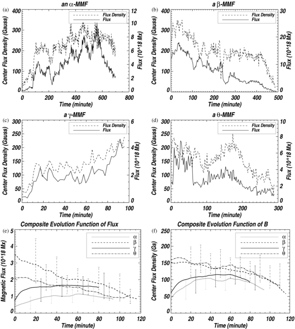
Figure 7. (a–d) The evolution of the magnetic flux (solid curve) and center flux density (dashed curve) of the four example MMFs shown in Figure 6 and 8. (e and f) The composite evolution functions of the magnetic flux (e) and flux density (f) of the four types of MMFs. Each composite plot shows a type of MMFs' most common pattern of evolution. The lifetime (amplitude) of a curve is the average lifetime (amplitude) of its type of MMFs.
Download figure:
Standard image High-resolution image
Figure 8. Sequences of magnetograms for two typical MMFs that formed in the moat. (a) The evolution of a γ-MMF. It emerged, moved southward, and merged into a bigger MMF. (b) A θ-MMF separated from another MMF of the same polarity, and decayed as it moved away from its mother MMF. These two MMFs' flux and flux density as functions of time are plotted in Figures 7(c) and (d).
Download figure:
Standard image High-resolution imageThe evolution curves of all the identified α- and β-MMFs are merged into two composite functions, applying the method described in Section 3.5. Figures 7(e) and (f) show the evolution of α- and β-composites. The β-composite (dashed curve) first appears with its maximum area and flux density, and it moves at a rather stable speed, but its magnetic field decreases all through its lifetime, until in the end it becomes too weak and small to be detected. On the other hand, the α-composite (dotted curve) evolves in a different way. Its initial magnetic flux is weak; in the first half of its life it increases in both flux density and area, and gains flux; after reaching its maximum flux it begins to diffuse. In the latter half of its life, although its area still increases gradually, the flux density keeps decreasing until the MMF disappears. The α-composite's velocity decreases faster than the β-composite's (Table 2).
4.4. MMFs Formed in Moat
Comparing the origins and displacements of penumbral MMFs (Figure 4(a)) to those of moat MMFs (Figure 4(b)) shows that, while the penumbral MMFs generally move along the radial direction, the moat MMFs' directions of motion are dispersed. Many of them move almost along the azimuthal direction; some γ-MMFs even move toward the parent sunspot instead of moving away from it as MMFs are traditionally defined.
Figure 8(a) shows a γ-MMF emerging in the moat, with no immediate connection to penumbral fibrils or other MMFs. Its initial magnetic flux was weak, as plotted in Figure 7(c). It moved southward along the azimuthal direction and gained flux. In about 1.5 hr, it moved 7'' on the solar surface at a speed of nearly 1 km s−1. Finally, it merged into another MMF with the same polarity. Similar to α-MMFs, γ-MMFs usually have weak initial flux, they gain flux in the rise phase and lose flux in the decline phase, as demonstrated by γ-MMF's composite evolution functions plotted in Figures 7(e) and (f) (solid curve).
The flux evolution of the θ-MMF in Figure 7(d) is opposite to that of the γ-MMF in Figure 7(c). As shown in Figure 8(b), it first separated from another MMF, then it lost flux as it moved slowly and eventually vanished in the moat. Similar to β-MMFs, strong initial flux, decreasing magnetic strength, and long lifetime are typical among θ-MMFs, as shown by the evolution of their composites (Figures 7(e) and (f), dash-dotted curve). θ-MMFs' speed and deceleration are the lowest among the four types (Table 2).
4.5. Dynamic MMFs in Moat
Types α, β, and γ each constitute about 30% of the total MMF flux, while θ-MMFs account for about 10%, as listed in Table 2. Figure 9(a) plots the amount of magnetic flux contributed by MMFs as functions of radial distance to penumbra. About 63% of the moat MMF fluxes are input by new emergence fluxes (α- and γ-MMFs). The remaining 37% are brought in by fragments from the penumbra (β-MMFs). θ-MMFs are results of fragmentation in the moat; they generally do not produce new flux input. Table 2 also lists the average values of several basic physics quantities of the four MMF sets. Comparing α- and γ-MMFs to β- and θ-MMFs, respectively, it can be noticed that MMFs produced by emergence have shorter lifetime and displacement, and are smaller in size and flux.
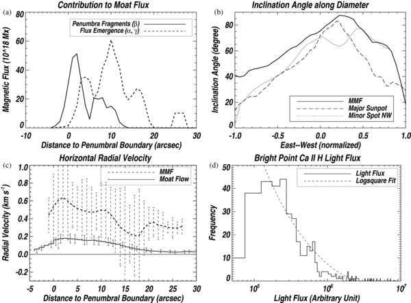
Figure 9. (a) MMFs' contribution to the moat flux in the observed region. About 37% of the moat fluxes were input by β-MMFs (solid curve) which are fragments from the penumbra. Majority of the moat flux input came from new flux emergences (dashed curve), both near the penumbra (α) and from the moat (γ). θ-MMFs do not bring new flux into the moat. (b) The solid curve shows the variation of field inclination angle along the diameter of a big isolated MMF. The dashed and dotted curves show the inclination angles across two of AR 10930's sunspots. The abscissa is the normalized distance to their flux centers. The inclination angles are measured from SP vector magnetograms. (c) The dashed curve is the average radial velocity of all identified MMFs as a function of the distance to the penumbra's outer boundary. The solid curve is the average horizontal radial flow velocity calculated using the LCT method on the region of interest. The error bars show the standard deviations. (d) The frequency distribution of the Ca ii H light fluxes of the identified bright points. The dashed curve is the logsquare fit.
Download figure:
Standard image High-resolution imageNearly half of the MMF population are γ-MMFs. Their paths cover a large part of the observed moat region (Figure 4(b)). Their average speed and deceleration are the highest among the four types. Some pairs of opposite-polarity γ-MMFs emerge in a relatively quiet vicinity, and move in opposite directions. Some of them emerge next to a relatively stationary magnetic feature of the opposite polarity, and move quickly toward another stationary feature of the same polarity. In several places, γ-MMFs are observed to emerge continuously and move on repeated paths. Section 4.7 introduces our observation of some moat flux emergences that are visible in low chromospheric filtergrams.
Within the moat region, the merging and flux cancellation between MMFs are frequent. For many MMFs, these are the dominant factors in their evolution. Their lifetime and flux growth/decay are determined not by the amount of initial flux, but by the number and flux of the magnetic elements they encounter. Among the MMFs that we traced, 41% disappeared due to flux cancellation with opposite-polarity magnetic elements, 37% merged with other same-polarity elements; only 22% of the MMFs disappeared without visible interaction with other magnetic elements. The total flux of positive MMFs (514 × 1018 Mx) is approximately equal to the total flux of negative MMFs (568 × 1018 Mx). This also indicates that flux cancellation is the main mechanism to make MMFs disappear and to maintain the flux balance of the moat. It is also possible that some flux diffused into tiny magnetic elements that are below the threshold of observation.
To demonstrate the dynamic nature of the moat, we examined the contacts made by a particular MMF with neighboring magnetic elements. Figure 10(a) shows the evolution of a big, negative polarity β-MMF. When it left the penumbra, its initial flux was only 3.2 × 10¹⁸ Mx. During its 14 hr long lifetime, it gained flux mostly by merging magnetic elements of the same polarity. It lost flux partly by fragmentation and partly by cancellation with opposite-polarity magnetic elements. We count 59 contact events during which the MMF gained flux. The total flux gained (56.9 × 10¹⁸ Mx) more than doubles the MMF's maximum flux (25.1 × 10¹⁸ Mx). These events are indicated by the black, inward pointing arrows in Figure 10(b). There were also 53 contact events in which the MMF lost 49.8 × 10¹⁸ Mx of flux in total. In Figure 10(b), they are indicated by the white arrows that point outward. The lower panel of Figure 10(c) compares the MMF's evolution of flux (solid curve) and flux density (dotted curve) with the Ca ii H light flux (dashed curve), where the light flux is the two-dimensional integration of image intensity in arbitrary units. The upper panel plots the amounts of flux gained (plus sign) and lost (minus sign) in the contact events. Some of the flux cancellation events appear as bright points on Ca ii H images. During the MMF's rise phase, the conglomeration process was the dominant mechanism, while flux cancellation was dominant in the decline phase.
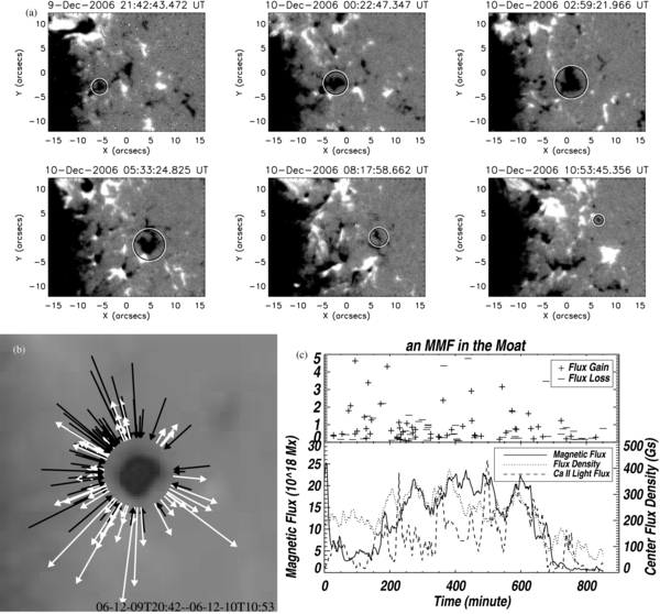
Figure 10. (a) The evolution of a negative polarity β-MMF. Its lifetime is nearly 14 hr. After leaving the penumbra, this MMF contacted with more than 100 smaller magnetic elements of both polarities. (b) The black (white) arrows indicate the contact events during which flux was gained (lost). The lengths of the arrows are proportional to the square root of the amount of flux transferred. The azimuth locations of the arrows indicate the approximate contact points. The background is a time-averaged, MMF-centered magnetogram. (c) Lower panel: the evolution of this MMF's flux (solid), flux density (dotted), and Ca ii H light flux (dashed, in arbitrary units). Upper panel: the plus and minus symbols indicate the flux gain and loss during the MMF's contacts with neighboring magnetic elements.
Download figure:
Standard image High-resolution imageA massive magnetic area left the major sunspot from the southwest side, as shown in Figure 6(a). It is a compact group of magnetic elements of various sizes. Due to the size and complexity of this region, the local magnetic elements are not counted as MMFs in this research.
4.6. Transverse Magnetic Field and Velocity Field
Figure 11 shows some sub-regions of the vector magnetograms obtained by SOT/SP spectrograph during the time of observation. The arrows are the transverse component of magnetic field vectors overlaying the vertical flux density. In Figure 11(a), at the places where MMFs meet with magnetic regions of opposite polarity, the transverse fields deviate from their directions in the neighboring regions and point to the contact area where the polarities meet.
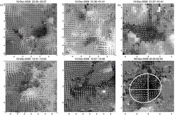
Figure 11. Arrows show the horizontal magnetic fields obtained by the SOT/SP spectrograph, overlaying the corresponding vertical fields. Each title shows the time duration when the spectrograph slit scanned the region. (a) Left and middle columns: in these regions MMFs collide with large magnetic areas of opposite polarity. The horizontal field points to the contact area. (b) Right column: the horizontal fields inside two big MMFs point toward their flux centers. In the lower panel, the ellipse is the least-square fit to the MMF's periphery, and the intersection of the horizontal and vertical lines is the flux center.
Download figure:
Standard image High-resolution imageOn SP vector magnetograms, we have selected a few isolated round-shaped magnetic elements. Their transverse field points to the flux center, as plotted in Figure 11(b), indicating that the magnetic field inside these MMFs is directed inward. The inclination angle i of their magnetic field to the photosphere has been measured along their diameters. At the MMFs' boundaries, the amplitude of the inclination angle |i| is between 10° and 40°. |i| increases as the field strength increases, while at the flux center the field is almost vertical. This profile is similar to the field orientation of sunspots. A sunspot's magnetic field also inclines toward the spot center, the zenith angle increases with the radial distance to spot center, and the magnetic field at the sunspot center is almost vertical (Lites & Skumanich 1990; Skumanich et al. 1994). As an example, the periphery and flux center of the MMF in the lower panel of Figure 11(b) are marked with a circle and a cross. The field inclination angle measured along its east–west diameter is plotted in Figure 9(b) (solid curve). The dashed and dotted curves show the variation of |i| along the major axes of two of AR 10930's sunspots.
Horizontal flow velocity field was computed with the local correlation tracking (LCT) technique using Stokes V/I line-of-sight magnetograms. A comparison between the time-averaged flow map (Figure 4(d)) and the G-band filtergrams shows that the flow basically follows the extension of penumbral fibrils, especially near the highly sheared polarity inversion lines (solid curve). In the regions where the flow speed is relatively high (delineated with dashed contours), the production of penumbral MMFs is intense (cf. Figures 4(a) and (b)).
Figure 9(c) compares the average radial velocity of the MMFs (dashed curve) with that of the moat flow field (solid curve), both as functions of the distance to penumbra outer boundary. It can be seen that the speed of MMFs (∼0.5 km s−1) is higher than the background flow speed (∼0.2 km s−1). The former is taken statistically by following individual features, while the latter by the local correlation technique. Although both methods provide a basic estimation on the outflow of magnetic flux from sunspots, the average speed measured from the manually selected MMF set is subject to bias in sample selection, because it is natural for the human eye to be "drawn to large, intense, rapidly moving features" (Brickhouse & Labonte 1988) and those leading ones in MMF groups. Also, the variances of MMFs' radial velocity (dashed error bars) are quite large, which is caused partly by the broad distribution of MMFs' speed, and partly by the randomness of γ-MMFs' directions of motion. At 0''–4'' outside of the penumbral boundary, the speed of MMFs is the highest; this agrees with Hurlburt & Rucklidge's (2000) observation of a "collar flow" right outside the penumbra. MMF's radial velocity reaches a minimum at about 17'' outside the penumbra.
4.7. Effects in Low Chromospheric Layers
Four hundred chromospheric bright points have been observed over the Ca ii H time series. Their locations have been marked in Figure 4(c). More than 80% of the observed bright points are associated with mixed-polarity groups of magnetic elements. The places where bright points frequently appear are close to the penumbral boundaries and have high-speed flow (cf. Figure 4(d)). Moreover, many MMFs are produced here and they frequently cancel with opposite-polarity elements.
The distribution of bright points' observed Ca ii H light flux is plotted in Figure 9(d). The histogram (solid curve) can be fitted with a logsquare model (dashed curve). The left end of the distribution function represents a large number of small bright points that release little light flux and energy.
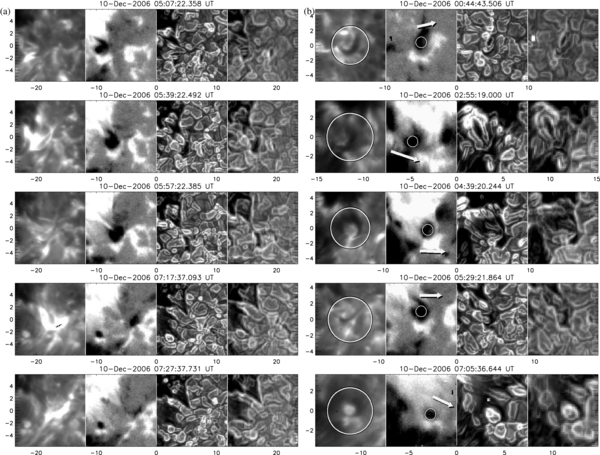
In Ca ii H images, many MMFs do not appear as identifiable features. However, quick emergence and fast motion of γ-MMFs are often visible. For example, the γ-MMF displayed in Figure 12(a) is small in size (∼1'') and flux (∼2 × 10¹⁸ Mx), but it can be clearly identified on Ca ii H and G-band filtergrams as a fast-moving bright point. It emerged next to one negative-polarity feature at the southwest corner of the small field of view, then it moved quickly toward a stationary positive polarity feature at the northeast corner, and finally merged with it. On the other hand, some big magnetic elements appear as dark patches on filtergrams, as displayed in Figure 12(b). On magnetograms they are about 4'' in size, and some of them became pores.
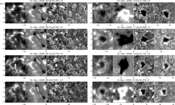
Figure 12. (a) A fast-moving γ-MMF (stamped with a circle) appeared as a bright dot in filtergrams. The arrows illustrate its direction of motion. In each panel are displayed simultaneous Ca ii H filtergram (first column from left), Fe i magnetogram (second column), and edge-enhanced G-band and Fe i filtergrams (third and fourth columns). (b) Examples of big (∼4'') magnetic elements. They appeared as dark patches on filtergrams.
Download figure:
Standard image High-resolution imageThe separation of magnetic elements of different polarities triggers short-timescale Ca ii H bright points, as illustrated by Figure 13(a). The elements' opposite directions of motion are illustrated by arrows. Bipolar flux emergence can also form mini dark filaments. In Figure 13(b), as the opposite-polarity MMF pairs emerge and move away from each other, small dark structures are formed and elongated.
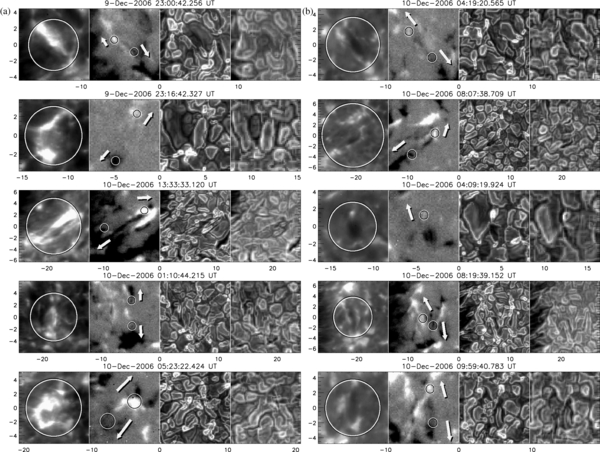
Figure 13. (a) Short-timescale, lengthened chromospheric bright points appeared in these emerging flux regions when magnetic elements of opposite polarities emerged and drifted apart. The speed of these magnetic elements and Ca ii H bright points was well above MMFs' average speed. (b) Elongated Ca ii H dark structures were formed as opposite-polarity magnetic elements moved away from each other.
Download figure:
Standard image High-resolution imageThe formation of penumbral MMFs is accompanied by Ca ii H bright points. Bright points are especially frequent and intense when a mixed group of α- and β-MMFs separate from the mother sunspots. Figure 14(a) is an example: as two bipolar MMFs leave the penumbra, more than ten Ca ii H bright points appeared within 2 hr. These bright points could be microflares.
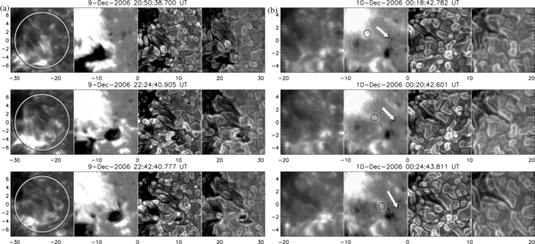
Figure 14. (a) During the formation of two bipolar penumbral MMF pairs, several micro dark filaments were formed. They connected the penumbra and the MMFs, and were stretched as the MMFs moved away from the penumbra. Several Ca ii H bright points appeared in this process. (b) Formation of a long dark structure on a short timescale. It was formed when a β-MMF (stamped with a circle) left the penumbra of a small positive polarity sunspot and moved quickly toward a negative polarity MMF in the moat. The lifetimes of the two filaments are about 3 hr (a) and 0.1 hr (b), respectively.
Download figure:
Standard image High-resolution imageDark chromospheric loop structures are observed when some penumbral MMFs move away from the penumbra. For each filament, one footpoint is on the parent sunspot, the other on a departing penumbral MMF. The filaments are stretched and elongated as the MMFs move away. Figure 14(a) shows the formation and elongation process of several dark filaments as bipolar penumbral MMFs left the penumbra. These filaments lasted for about 3 hr. The filament in Figure 14(b) was formed when a fast-moving β-MMF moved away from the penumbra to join with a magnetic element of opposite polarity. The lifetime of this filament is less than ten minutes.
The collisions of opposite-polarity magnetic elements frequently produce bright points. For instance, in Figure 15(a), as a negative-polarity MMF moved westward, it encountered several positive-polarity MMFs and triggered several microflares. During this process the flux of this negative-polarity MMF decreased rapidly and finally disappeared. Flux cancellation events are probably responsible for most of the bright points in the moat.
Figure 15. (a) Temporal evolutions of a negative-polarity MMF's collision with neighboring positive-polarity MMFs. The flux cancellation process was accompanied by several Ca ii H bright points. (b) Horn-shaped dark structures were formed during the collision between opposite-polarity MMFs. The arrows indicate the directions of motion of the negative-polarity MMFs (circled).
Download figure:
Standard image High-resolution image
In some cases, collisions of opposite-polarity magnetic elements form chromospheric dark structures. Figure 15(b) shows five horn-shaped dark chromospheric structures. They were formed during the collision between a moving negative polarity MMF and a neighboring positive polarity magnetic element. These micro-filaments usually have uneven footpoints: one is substantially bigger than the other.
Granules and filigrees can be clearly identified in edge-enhanced G-band time sequences. However, their form and location frequently change on a timescale shorter than the time cadence of the instrument (120 s), which makes it difficult to follow their evolution. Also, their vast numbers suggest that, in order to study these features statistically, an automated feature-recognition procedure should be utilized.
5. DISCUSSION AND CONCLUSION
After careful examination of 240 MMFs in the filter magnetograms and 400 Ca ii H bright points in the images of Hinode/SOT, we present the following major results regarding MMFs' origins, motion, evolution patterns, and their impacts on lower chromospheric layers:
- 1.Fifty percent of MMFs originate from or among the penumbra fibrils. They move outward mostly along the radial direction after they leave the penumbra. Many of them have precursors within the penumbra. Fifty percent of MMFs emerge in the moat, whose orientations of motion are random to some extent. MMFs' average radial velocity more than doubles the background moat flow speed, it reaches maximum at 0''–4'' outside the penumbra, and it reaches the minimum at about 17'' outside the penumbra. MMFs reach their maximum velocity during the first half of their life and afterward decelerate. While there are bipolar MMFs that originate from the penumbra and move outward together, bipolar emergences within the moat frequently produce MMF pairs that move apart.
- 2.The evolution of MMFs that are fragments from a parent magnetic area is usually a decay and fragmentation process. Their decay process starts once they become isolated features. The fluxes of newly emerged MMFs are usually smaller than those separated from other magnetic areas. During their rise phase, their flux and size increase through new flux emergence or merging other magnetic elements. In the latter decline phase, they lose flux by flux cancellation and fragmentation. New emergences constitute about 63% of the moat flux. Merging and flux cancellation between MMFs are very frequent in the moat, and they determine the evolution of MMFs.
- 3.Most of the Ca ii H bright points are caused by cancellations between opposite-polarity magnetic areas. Bright points may also be triggered by MMFs' severance from the penumbra, fragmentation, and merging. Fast-moving moat MMFs appear as bright dots in the low chromosphere, while big magnetic elements appear as dark patches in filtergrams. Elongated or horn-shaped chromospheric micro-filaments are produced during the separation or cancellation process between opposite-polarity MMFs.
The distributions of MMFs' magnetic flux, area, lifetime, and displacement are nearly lognormal, which suggest the existence of a large number of small, short-lived, even indistinguishable MMFs. This is consistent with Hagenaar & Shine's (2005) observation. Interestingly, the size distribution of sunspots' umbrae is well described by a lognormal function (Bogdan et al. 1988). These might imply that the fragmentation process exists in flux tubes of very different scales.
We measured MMF's magnetic field under the assumption that the distribution of a magnetic element's flux along its radius is Gaussian, and the composite profile of MMFs' flux density (Figure 5(b)) is indeed Gaussian. Lamb et al. (2010) also find the two-dimensional distribution of a magnetic element's flux core to be Gaussian. But it is yet to be determined whether this normal distribution is an intrinsic nature of MMFs, or it is merely an accumulation of the randomness of MMFs' shape.
The distinct origins of the α- and β-MMFs can be explained by the "uncombed" model (Solanki & Montavon 1993; Solanki 2003). The more vertical flux tubes in the "interlocked" penumbral structure leave the penumbra and appear in magnetograms as β-MMFs which have the same polarity as the sunspot. α-MMFs may have been formed by those more horizontal penumbral fibrils; they plunge into the photosphere from above and form footpoints that have the opposite polarity to the penumbra. It needs further observation to investigate the association between α/β-MMFs and dark/bright penumbral fibrils.
In the moat, the interactions between magnetic elements are frequent and active, and they determine MMFs' evolution. Most of the MMFs disappear by merging or flux cancellation, as shown by our examination of a particular MMF in Figure 10. It is noticed that γ-MMFs occupy a substantial portion of our sample pool and frequently appear with a quick emergence. They emerge in the moat and have no apparent connection to other magnetic objects. Lamb et al. (2008), Parnell et al. (2009), and Iida et al. (2012) explained unipolar appearances with asymmetric emergences, i.e., bipolar emergences with one polarity less detectable. They also argued that, in producing photospheric magnetic features, the coalescence of previously unobservable flux into observable concentrations is more important than bipolar emergence. This scenario is consistent with our observations that flux emergence, flux cancellation, and merging are very frequent in the moat.
Within the moat there are numerous short-timescale small flux emergences. Observations of their emergence, merging, and disappearance would help to explain the evolution of MMFs. However, we were not able to observe much detail about them, partly due to the fact that these elements evolve on a timescale shorter than the time cadence of the NFI (∼120 s), making it difficult to connect the small-scale magnetic configurations of an image with its adjacent frames. The observation of these flux emergences could be performed better with telescopes that obtain magnetograms at a time cadence one or two orders of magnitudes lower than the NFI. It could be an interesting observational topic in the future.
We are especially grateful to comrades Jiangtao Su, Xiao Yang, and Xianyong Bai for carefully reading and commenting on the manuscript. Thanks are also due to an anonymous referee for comments and suggestions to improve this paper. This study is supported by National Basic Research Program of China, grant 2011CB811400, National Natural Science Foundation of China, grants 10733020, 10921303, 41174153, and Specialized Research Fund for State Key Laboratories. Hinode is a Japanese mission developed and launched by ISAS/JAXA, with NAOJ as domestic partner and NASA and STFC (UK) as international partners. It is operated by these agencies in co-operation with ESA and NSC (Norway). This research has made use of IDL, GDL, Gnu R, Mathematica, SolarSoft (Freeland & Handy 1998), and Ubuntu Linux.
Footnotes
- 1
Developed under the Community Spectro-polarimetric Analysis Center (CSAC) initiative at the National Center for Atmospheric Research, Boulder, CO, USA; http://sot.lmsal.com/data/sot/level2hao_new/.