


ABSTRACT
We present the results of a search for extended X-ray sources and their corresponding galaxy groups from 800 ks Chandra coverage of the All-wavelength Extended Groth Strip International Survey (AEGIS). This yields one of the largest X-ray-selected galaxy group catalogs from a blind survey to date. The red-sequence technique and spectroscopic redshifts allow us to identify 100% of reliable sources, leading to a catalog of 52 galaxy groups. These groups span the redshift range z ∼ 0.066–1.544 and virial mass range M200 ∼ 1.34 × 10¹³–1.33 × 10¹⁴ M☉. For the 49 extended sources that lie within DEEP2 and DEEP3 Galaxy Redshift Survey coverage, we identify spectroscopic counterparts and determine velocity dispersions. We select member galaxies by applying different cuts along the line of sight or in projected spatial coordinates. A constant cut along the line of sight can cause a large scatter in scaling relations in low-mass or high-mass systems depending on the size of the cut. A velocity-dispersion-based virial radius can cause a larger overestimation of velocity dispersion in comparison to an X-ray-based virial radius for low-mass systems. There is no significant difference between these two radial cuts for more massive systems. Independent of radial cut, an overestimation of velocity dispersion can be created in the case of the existence of significant substructure and compactness in X-ray emission, which mostly occur in low-mass systems. We also present a comparison between X-ray galaxy groups and optical galaxy groups detected using the Voronoi–Delaunay method for DEEP2 data in this field.
Export citation and abstract BibTeX RIS
1. INTRODUCTION
Groups of galaxies are important laboratories for the study of galaxy evolution and formation. They are in the stage between the field and the densest environment in the universe, massive clusters (Zabludoff & Mulchaey 1998), and as many as 50%–70% of all galaxies reside in galaxy groups (Turner & Gott 1976; Geller & Huchra 1983; Eke et al. 2005).
It is valuable to study galaxy groups over a range of cosmic time to understand the effect of the group environment on the galaxy population. Several efforts have been made to identify groups and clusters up to redshift one and beyond (e.g., Stanford et al. 2006; Eisenhardt et al. 2008; Bielby et al. 2010; Tanaka et al. 2010). The faint X-ray emission and low galaxy number densities of galaxy groups make such environments difficult to distinguish from the field compared to massive galaxy clusters at higher redshifts. We have relatively good knowledge and samples of galaxy groups in the local universe (e.g., Mulchaey & Zabludoff 1998) but there is a lack of similar samples of galaxy groups that have both sufficiently deep X-ray data and counterparts with optical spectroscopy at high redshift. In the presence of advances in deep X-ray surveys, extended X-ray emission provides a reliable signal for detecting such environments at high redshifts.
There are a number of different methods for detecting groups of galaxies: searches in optical data via the red-sequence method (e.g., Gladders & Yee 2005; Koester et al. 2007), the Sunyaev–Zeldovich (SZ) effect on the cosmic microwave background, CMB (e.g., Sunyaev & Zeldovich 1970, 1972; Carlstrom et al. 2002; LaRoque et al. 2003; Benson et al. 2004; Staniszewski et al. 2009), X-ray emission from hot intracluster gas (e.g., Boehringer et al. 2000; Hasinger et al. 2001; Vikhlinin et al. 2009; Finoguenov et al. 2010), cosmic shear due to weak gravitational lensing maps (e.g., Miyazaki et al. 2007; Massey et al. 2007), and spectroscopic group samples (e.g., Gerke et al. 2012; Miller et al. 2005; Knobel et al. 2009, 2012). While spectroscopic surveys reveal the largest and deepest group catalogs, the detection of group X-ray emission has been proven to ensure that objects are virialized, and with the deepest X-ray survey available to date, the limits to which X-ray emission can be detected are reaching the level of low-mass groups. Moreover, compared to shear maps, X-rays probe a wider range in mass and redshift (Leauthaud et al. 2010).
In this paper, with recent deep Chandra data (K. Nandra et al., in preparation), we search for galaxy groups in a wide range of redshifts in the Extended Groth Strip (EGS). In previous work, searching for galaxy groups in Chandra data with a nominal exposure time of 200 ks and ∼0.67 deg2 coverage of the EGS field yielded a discovery of seven high-significance galaxy groups in this field (Jeltema et al. 2009). We now add new Chandra data with approximately 800 ks exposure time covering ∼0.25 deg2 field; see Figure 1. Furthermore, EGS is one of the four fields in the Deep Extragalactic Evolutionary Probe 2 (DEEP2) spectroscopy survey (Davis et al. 2003; Newman et al. 2012), and it is the only field that has been targeted for extensive spectroscopic data in DEEP3 (Cooper et al. 2011, 2012). The DEEP2 and DEEP3 coverage of EGS is magnitude-limited but not color-selected, yielding a large sample of spectroscopic galaxies at all redshifts, enabling us to identify our groups optically and determine their velocity dispersions.
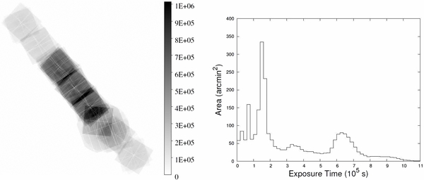
Figure 1. Exposure map (left panel) and the distribution of exposure time (right panel) in Chandra and XMM coverage of EGS.
Download figure:
Standard image High-resolution imageThis paper is laid out as follows: Section 2 presents a brief description of AEGIS and our data, while Section 3 describes our method for group identification. We present our identified group catalog in Section 4. In Section 5, we present spectroscopic group membership and the dynamical properties of the groups. We make a comparison between the X-ray groups and optical groups, which are identified from the Voronoi–Delaunay method (VDM) in the DEEP2 spectroscopic data set in Section 6. Throughout this paper a ΛCDM cosmology with Ωm = 0.27, ΩΛ = 0.73, and H0 = 100 h km s−1 Mpc−1 where h = 0.71 is assumed.
2. THE AEGIS SURVEY
AEGIS brings together deep imaging data from X-ray to radio wavelengths and optical spectroscopy over a large area (0.5–1 deg2). This survey includes Chandra/ACIS X-ray (0.5–10 keV), GALEX ultraviolet (1200–2500 Å), CFHT/MegaCam Legacy Survey optical (3600–9000 Å), CFHT/CFH12K optical (4500–9000 Å), Hubble Space Telescope/ACS optical (4400–8500 Å), Palomar/WIRC near-infrared (1.2–2.2 μm), Spitzer/IRAC mid-infrared (3.6, 4.5, 5.8, and 8 μm), VLA radio continuum (6–20 cm), and a large spectroscopic data set using the DEIMOS spectrograph on the Keck II 10 m telescope in an area with low extinction and low Galactic and zodiacal infrared emission (Davis et al. 2007). In the following section, we will describe the various data sets used in this analysis.
2.1. X-Ray Data
Our very deep Chandra survey used the Advanced CCD Imaging Spectrometer (ACIS-I) in three contiguous fields covering a total area of 0.25 deg2 (K. Nandra et al., in preparation) and a series of eight pointings covering a total area of approximately 0.67 deg2 in EGS. Laird et al. (2009) provided the details for the latter survey and the X-ray point source catalog. The total exposure time is approximately 3.4 Ms with a nominal exposure of 800 ks in each of the three central fields.
We also used the XMM-Newton observations of the field (ObsIDs 0127921001, 0127921101, 0127921201, and 0503960101), which were processed and co-added following the prescription of Bielby et al. (2010). The total time of XMM observations is 100 ks and its contribution to the final coverage can be seen in Figure 1 as a somewhat round area in the southern part of the survey. Here, we present the X-ray extended source catalog based on the Chandra and XMM observations in EGS.
In the Chandra analysis, we applied a conservative event screening and modeling of the quiescent background. We filtered the light curve events using the lc clean tool in order to remove normally undetected particle flares. The background model maps have been evaluated with the prescription of Hickox & Markevitch (2006). We estimated the particle background by using the ACIS stowed position20 observations and by rescaling them using the ratio of the hard band (9.5–12 keV) fluxes. The cosmic background flux has been evaluated by subtracting the particle background maps from the real data and masking the area occupied by the detected sources. We applied the method used in Finoguenov et al. (2009) to search for extended sources and, as a result, we found 56 extended sources in the EGS strip. Briefly, X-ray data have been obtained from X-ray mosaics made from the co-addition of the XMM-Newton and Chandra data. After background subtraction and point source removal for each observation and each instrument were done separately, the residual images were co-added, taking into account the difference in the sensitivity of each instrument to produce a joint exposure map. To detect the sources, we ran a wavelet detection at 32'' and 64'' spatial scales, similar to the procedure described in Finoguenov et al. (2007, 2009).
2.2. Photometric Data
The EGS field is located at the center of the third wide field of the Canada–France–Hawaii Telescope Legacy Survey (CFHTLS-Wide3, W3)21, which is covered in u*, g', r', i', and z' filters down to i' = 24.5 with photometric data for 366,190 galaxies (Brimioulle et al. 2008). The photometric redshifts for the wide field are derived from the photo-z code of Bender et al. (2001). The EGS field also contains the CFHTLS Deep 3 field (Davis et al. 2007), which covers 1 deg2 with ugriz imaging to depths ranging from 25.0 in z to 27 in g. In this work, we have used the T0006 release of the CFHTLS Deep data.22 The CFHTLS Deep field also contains near-infrared coverage in the JHK bands via the WIRCam Deep Survey (WIRDS; Bielby et al. 2012). This covers 0.4 deg2 of the D3 field and provides deep imaging to ∼24.5 (AB) in the three NIR bands. The photometric redshifts in the region covered by the NIR data were determined using the Le Phare code as described in Bielby et al. (2010).
2.3. Spectroscopic Data
The DEEP2 Redshift Survey has targeted ∼3.5 deg2 within four fields on the sky using the DEIMOS multi-object spectrograph (Faber et al. 2003) on the Keck II Telescope (Davis et al. 2003). All the DEEP2 targets have 18.5 ⩽ R ⩽ 24.1. The EGS is one of these four fields. Compared to other DEEP2 fields, EGS spectroscopy is magnitude-limited, but not color-selected, giving one the advantage of being able to obtain a sample of galaxies at all redshifts (Davis et al. 2007). In addition, this region of sky has been targeted for extensive spectroscopy with DEEP3 (Cooper et al. 2011, 2012). The DEEP2 and DEEP3 catalogs have about 23,822 unique objects in total (with −2 ⩽ redshift quality ⩽ 4) and 16,857 objects with reliable redshifts (with redshift quality ⩾ 3). In addition to DEEP2 and DEEP3, EGS is located in the Sloan Digital Sky Survey23 (SDSS) coverage, so we have additional spectra for our low-redshift galaxies. We also used redshifts of spectroscopic galaxies obtained from follow-up observations of the DEEP2 sample with the Hectospec spectrograph on the Multiple Mirror Telescope (MMT; Coil et al. 2009).
3. OPTICAL IDENTIFICATION
To identify the groups in redshift space, we used galaxies with good redshift quality in DEEP2 and DEEP3 to construct our initial redshift catalog. Using this catalog, imaging data, and position of X-ray extended sources, we assigned a redshift to each X-ray source visually, where the spatial distribution of galaxies in the sky coincides with the X-ray emission. For those sources for which we found more than one counterpart and the X-ray shape allows us to securely separate the contribution from several counterparts, we define a new ID in our X-ray catalog. The detected source areas are searched for flux extension down to a 90% confidence level, which is subsequently used for flux estimation.
We also used the refined red-sequence technique, described in Finoguenov et al. (2010), to confirm the overdensity of red galaxies within or near those X-ray sources for which we have a lack of spectroscopic data. In brief, we selected galaxies with |z − zphot| < 0.2 and within a physical distance of 0.5 Mpc from the center of X-ray emission at the given redshift. Then, using a Gaussian weight, we count the galaxies around the model red sequence and find overdensities. Since different observed colors are sensitive to red galaxies at different redshifts, we adopt the following combination of colors and magnitudes.
For those groups that lie in D3 field in CFHTLS :
0.0 < z < 0.3 : u* − r' color and r' magnitude,
0.3 < z < 0.6 : g' − i' color and i' magnitude,
0.6 < z < 1.0 : r' − z' color and z' magnitude,
1.0 < z < 1.5 : i' − J color and J magnitude,
1.5 < z < 2.0 : z' − Ks color and Ks magnitude.
For those in the W3 field:
0.0 < z < 0.3 : u* − r' color and r' magnitude,
0.3 < z < 0.6 : g' − i' color and i' magnitude,
0.6 < z : r' − z' color and z' magnitude.
We note that Bielby et al. (2010) mistakenly quoted their filter combinations to identify red-sequence signals. They used the same filters as in our D3 field. Using the red-sequence technique and the spectroscopic data, we identify redshifts for 52 extended X-ray sources. We have spectroscopic redshifts for 49 galaxy groups and more than 2 spectroscopic members for 46 galaxy groups.
We also assigned a flag to each extended source that describes the quality of the identification. Flag = 1 indicates a confident redshift assignment, significant X-ray emission, and good centering, while Flag = 2 indicates the centering has a large uncertainty. In the cases where a single X-ray source has been matched to several optical counterparts, the assigned flag is equal to 2 or larger. For Flag = 3, we have no spectroscopic confirmation but good centering, and for Flag = 4, we have unlikely redshifts due to the lack of spectroscopic objects and red galaxies and also a large uncertainty in centering. We assigned Flag = 5 to the 13 unreliable cases for which we could not identify any redshift. They can be split into the following categories.
Some of the X-ray extended sources do not have spherical and symmetric morphologies and some exhibit a secondary peak in X-ray distribution. Initially, we expected these results from overlapping systems, but visual inspection of the optical data and the red-sequence method indicate a single significant group for some of these. Thus, we classify the second shallow peak in the X-rays as a substructure inside those real groups. Furthermore, sources on the edge of X-ray coverage with a low signal-to-noise ratio and no optical counterparts can be explained as having residual background in the images or bright X-ray clusters outside the field of view. We note that two RCS-2 clusters (Gilbank et al. 2011) are located 10' west from the edge of the survey. In the few cases of bright stars near the X-ray emission, we could not match galaxy counterparts to the extended emission. We assigned Flag = 5 to all of these cases and they are not included in the final sample.
4. A CATALOG OF IDENTIFIED X-RAY GROUPS
In this section, we describe our catalog of 52 X-ray galaxy groups detected in AEGIS (Table 1). The group identification number, R.A., and decl. of the peak of X-ray emission in Equinox J2000.0 are listed in Columns 1, 2, and 3. In Column 4, the mean of the red-sequence redshifts, which is substituted with the median of the spectroscopic redshifts in cases where there is a spectroscopic redshift determination for the group member galaxies is listed. We provide the group flux in the 0.5–2 keV band in Column 5 with the corresponding 1σ error. The rest-frame luminosity in the 0.1–2.4 keV is given in Column 6. Column 7 lists the estimated total mass, M200, computed following Leauthaud et al. (2010) and assuming a standard evolution of scaling relations: M200Ez = f(LxE−1z) where Ez = (ΩM(1 + z)3 + ΩΛ)1/2. The corresponding r200, M200 = (4/3)πr3200(200ρcritical), in arcminutes is given in Column 8. Column 9 lists the flag from our identification, as described in Section 3. The number of spectroscopic member galaxies inside r200 is given in Column 10 (see Section 5). Column 11 lists the flux significance, which provides insight into the reliability of both the source detection and the identification. The velocity dispersion estimated from X-ray luminosities is given in Column 12.
Table 1. AEGIS X-Ray Galaxy Groups
| ID | R.A. | Decl. | z | Flux | LX | M200 | r200 | Flag | N(z) | Flux | σX |
|---|---|---|---|---|---|---|---|---|---|---|---|
| (10−14 erg cm−2 s−1) | (1042 erg s−1) | (1013 M☉) | (arcmin) | Significance | |||||||
| EGSXG J1414.8+5209 | 213.71657 | 52.16481 | 0.455 | 0.50 ± 0.08 | 6.35 ± 0.98 | 4.61 ± 0.44 | 1.8 | 4 | 3 | 6.50 | 325 |
| EGSXG J1414.8+5212 | 213.71946 | 52.21343 | 0.301 | 0.38 ± 0.09 | 1.76 ± 0.43 | 2.32 ± 0.35 | 2.0 | 2 | 3 | 4.11 | 251 |
| EGSXG J1415.0+5204a | 213.76555 | 52.07685 | 0.074 | 2.77 ± 0.33 | 0.56 ± 0.07 | 1.34 ± 0.10 | 5.7 | 1 | 28 | 8.49 | 202 |
| EGSXG J1415.4+5220a | 213.85106 | 52.34112 | 0.074 | 4.22 ± 0.46 | 0.84 ± 0.09 | 1.73 ± 0.12 | 6.2 | 2 | 19 | 9.19 | 220 |
| EGSXG J1415.6+5221 | 213.91018 | 52.36540 | 0.622 | 0.33 ± 0.07 | 9.20 ± 1.94 | 5.01 ± 0.65 | 1.5 | 4 | 9 | 4.73 | 345 |
| EGSXG J1416.1+5224 | 214.02791 | 52.41598 | 0.571 | 0.13 ± 0.07 | 3.19 ± 1.67 | 2.67 ± 0.82 | 1.3 | 1 | 6 | 1.92 | 277 |
| EGSXG J1416.2+5205a | 214.07123 | 52.09987 | 0.832 | 0.91 ± 0.13 | 46.87 ± 6.79 | 11.68 ± 1.06 | 1.6 | 2 | 1 | 6.90 | 475 |
| EGSXG J1416.3+5213 | 214.07507 | 52.22752 | 0.641 | 0.12 ± 0.04 | 4.02 ± 1.46 | 2.90 ± 0.64 | 1.2 | 4 | 7 | 2.76 | 288 |
| EGSXG J1416.3+5229 | 214.07862 | 52.49943 | 0.356 | 0.36 ± 0.08 | 2.46 ± 0.55 | 2.74 ± 0.38 | 1.8 | 2 | 8 | 4.44 | 268 |
| EGSXG J1416.3+5214 | 214.08759 | 52.23544 | 0.366 | 0.25 ± 0.06 | 1.83 ± 0.43 | 2.25 ± 0.32 | 1.7 | 4 | 8 | 4.27 | 251 |
| EGSXG J1416.4+5227 | 214.12227 | 52.45173 | 0.837 | 0.30 ± 0.06 | 17.81 ± 3.26 | 6.26 ± 0.71 | 1.3 | 1 | 7 | 5.46 | 386 |
| EGSXG J1416.6+5228 | 214.15991 | 52.47882 | 0.812 | 0.09 ± 0.04 | 5.94 ± 2.34 | 3.17 ± 0.75 | 1.1 | 3 | 5 | 2.54 | 307 |
| EGSXG J1416.6+5222 | 214.17417 | 52.37189 | 0.510 | 0.15 ± 0.04 | 2.63 ± 0.79 | 2.50 ± 0.45 | 1.4 | 2 | 5 | 3.35 | 267 |
| EGSXG J1416.6+5229 | 214.17480 | 52.48355 | 0.238 | 0.33 ± 0.09 | 0.87 ± 0.23 | 1.56 ± 0.25 | 2.1 | 4 | 6 | 3.82 | 218 |
| EGSXG J1416.8+5210 | 214.20403 | 52.17700 | 0.900 | 1.04 ± 0.15 | 63.55 ± 8.95 | 13.33 ± 1.17 | 1.6 | 3 | 0 | 7.10 | 503 |
| EGSXG J1417.0+5226 | 214.25416 | 52.44758 | 1.023 | 0.08 ± 0.02 | 10.89 ± 2.90 | 3.85 ± 0.63 | 1.0 | 1 | 5 | 3.75 | 340 |
| EGSXG J1417.2+5215 | 214.31665 | 52.25140 | 0.470 | 0.20 ± 0.05 | 2.82 ± 0.72 | 2.71 ± 0.42 | 1.5 | 3 | 0 | 3.95 | 273 |
| EGSXG J1417.3+5235 | 214.34115 | 52.59349 | 0.236 | 0.27 ± 0.05 | 0.73 ± 0.14 | 1.39 ± 0.17 | 2.1 | 1 | 9 | 5.07 | 210 |
| EGSXG J1417.4+5237 | 214.37150 | 52.63047 | 0.355 | 0.39 ± 0.05 | 2.66 ± 0.34 | 2.88 ± 0.23 | 1.9 | 1 | 14 | 7.72 | 273 |
| EGSXG J1417.5+5238 | 214.38305 | 52.63655 | 0.717 | 0.29 ± 0.06 | 11.61 ± 2.36 | 5.32 ± 0.67 | 1.4 | 2 | 13 | 4.93 | 358 |
| EGSXG J1417.5+5232 | 214.38819 | 52.53527 | 0.985 | 0.25 ± 0.03 | 22.59 ± 2.87 | 6.35 ± 0.51 | 1.2 | 2 | 6 | 7.87 | 399 |
| EGSXG J1417.7+5228 | 214.44405 | 52.47140 | 0.995 | 0.16 ± 0.04 | 16.36 ± 4.08 | 5.12 ± 0.79 | 1.1 | 1 | 5 | 4.01 | 372 |
| EGSXG J1417.7+5241a | 214.44751 | 52.69237 | 0.066 | 3.92 ± 0.24 | 0.62 ± 0.04 | 1.43 ± 0.06 | 6.5 | 1 | 23 | 16.27 | 206 |
| EGSXG J1417.9+5226 | 214.47592 | 52.43701 | 0.684 | 0.13 ± 0.03 | 5.04 ± 1.30 | 3.22 ± 0.51 | 1.2 | 4 | 3 | 3.88 | 301 |
| EGSXG J1417.9+5235 | 214.48176 | 52.58382 | 0.683 | 0.27 ± 0.03 | 9.76 ± 1.04 | 4.92 ± 0.33 | 1.4 | 1 | 11 | 9.42 | 346 |
| EGSXG J1417.9+5225 | 214.48632 | 52.42462 | 0.995 | 0.10 ± 0.03 | 11.68 ± 3.58 | 4.13 ± 0.77 | 1.0 | 3 | 5 | 3.26 | 347 |
| EGSXG J1417.9+5231 | 214.49046 | 52.52231 | 0.661 | 0.16 ± 0.03 | 5.52 ± 0.93 | 3.49 ± 0.37 | 1.3 | 1 | 6 | 5.91 | 308 |
| EGSXG J1418.0+5222 | 214.50330 | 52.36890 | 0.950 | 0.22 ± 0.04 | 18.79 ± 3.81 | 5.83 ± 0.73 | 1.2 | 3 | 0 | 4.94 | 386 |
| EGSXG J1418.1+5225 | 214.52697 | 52.41944 | 0.548 | 0.21 ± 0.05 | 4.40 ± 0.96 | 3.35 ± 0.45 | 1.4 | 1 | 3 | 4.59 | 297 |
| EGSXG J1418.3+5227 | 214.59199 | 52.45022 | 0.281 | 0.27 ± 0.06 | 1.08 ± 0.25 | 1.73 ± 0.24 | 1.9 | 2 | 7 | 4.36 | 227 |
| EGSXG J1418.5+5252 | 214.62561 | 52.86899 | 1.025 | 0.10 ± 0.03 | 12.31 ± 3.83 | 4.15 ± 0.79 | 1.0 | 2 | 1 | 3.21 | 349 |
| EGSXG J1418.8+5248 | 214.70147 | 52.80696 | 0.741 | 0.06 ± 0.02 | 3.37 ± 1.07 | 2.36 ± 0.45 | 1.0 | 1 | 4 | 3.15 | 274 |
| EGSXG J1419.0+5236 | 214.76363 | 52.61357 | 0.550 | 0.45 ± 0.04 | 9.25 ± 0.85 | 5.38 ± 0.31 | 1.7 | 1 | 11 | 10.86 | 348 |
| EGSXG J1419.0+5257 | 214.76810 | 52.95626 | 0.656 | 0.32 ± 0.04 | 10.37 ± 1.15 | 5.24 ± 0.36 | 1.5 | 1 | 16 | 9.02 | 352 |
| EGSXG J1419.2+5255 | 214.82121 | 52.91803 | 0.782 | 0.14 ± 0.02 | 7.51 ± 1.29 | 3.79 ± 0.41 | 1.2 | 3 | 10 | 5.80 | 324 |
| EGSXG J1419.4+5301 | 214.85110 | 53.02358 | 0.745 | 0.15 ± 0.03 | 6.95 ± 1.52 | 3.74 ± 0.50 | 1.2 | 1 | 6 | 4.57 | 320 |
| EGSXG J1419.6+5251 | 214.91782 | 52.85103 | 0.670 | 0.14 ± 0.03 | 4.99 ± 1.24 | 3.24 ± 0.50 | 1.2 | 1 | 6 | 4.01 | 301 |
| EGSXG J1419.7+5246 | 214.93393 | 52.77711 | 0.784 | 0.18 ± 0.06 | 9.53 ± 3.10 | 4.41 ± 0.87 | 1.2 | 1 | 6 | 3.07 | 340 |
| EGSXG J1419.8+5300 | 214.96203 | 53.01138 | 0.744 | 0.19 ± 0.03 | 8.85 ± 1.29 | 4.36 ± 0.40 | 1.3 | 1 | 14 | 6.87 | 337 |
| EGSXG J1420.0+5258 | 215.00399 | 52.97709 | 0.454 | 0.15 ± 0.03 | 1.91 ± 0.39 | 2.14 ± 0.27 | 1.4 | 1 | 7 | 4.95 | 251 |
| EGSXG J1420.0+5306 | 215.00462 | 53.11241 | 0.200 | 0.48 ± 0.05 | 0.85 ± 0.10 | 1.59 ± 0.11 | 2.5 | 2 | 19 | 8.93 | 218 |
| EGSXG J1420.2+5308 | 215.06885 | 53.13864 | 1.105 | 0.13 ± 0.04 | 18.62 ± 5.14 | 5.03 ± 0.85 | 1.0 | 2 | 3 | 3.63 | 378 |
| EGSXG J1420.4+5311 | 215.12046 | 53.19035 | 1.544 | 0.18 ± 0.04 | 54.10 ± 13.11 | 6.80 ± 1.01 | 0.9 | 2 | 3 | 4.13 | 451 |
| EGSXG J1420.5+5308a | 215.14733 | 53.13952 | 0.734 | 0.41 ± 0.04 | 17.19 ± 1.75 | 6.74 ± 0.43 | 1.5 | 1 | 17 | 9.84 | 388 |
| EGSXG J1420.8+5306 | 215.20148 | 53.10867 | 0.355 | 0.35 ± 0.05 | 2.41 ± 0.36 | 2.71 ± 0.25 | 1.8 | 2 | 14 | 6.73 | 267 |
| EGSXG J1421.3+5308 | 215.32631 | 53.14764 | 0.351 | 0.26 ± 0.08 | 1.72 ± 0.51 | 2.19 ± 0.39 | 1.7 | 2 | 7 | 3.40 | 249 |
| EGSXG J1421.4+5308 | 215.34650 | 53.13477 | 0.201 | 0.54 ± 0.11 | 0.97 ± 0.20 | 1.72 ± 0.21 | 2.5 | 2 | 15 | 4.96 | 224 |
| EGSXG J1421.5+5302 | 215.38609 | 53.04315 | 0.677 | 0.53 ± 0.18 | 17.62 ± 6.11 | 7.22 ± 1.52 | 1.6 | 2 | 5 | 2.88 | 393 |
| EGSXG J1422.0+5328 | 215.51144 | 53.47268 | 0.357 | 0.51 ± 0.19 | 3.54 ± 1.30 | 3.46 ± 0.77 | 2.0 | 1 | 6 | 2.71 | 290 |
| EGSXG J1422.6+5321a | 215.66020 | 53.36037 | 0.768 | 0.36 ± 0.10 | 16.95 ± 4.73 | 6.47 ± 1.10 | 1.4 | 1 | 9 | 3.58 | 388 |
| EGSXG J1423.0+5326 | 215.76783 | 53.44306 | 0.615 | 0.28 ± 0.11 | 7.66 ± 2.94 | 4.49 ± 1.04 | 1.5 | 2 | 3 | 2.60 | 332 |
| EGSXG J1423.6+5328a | 215.92348 | 53.47078 | 1.132 | 0.27 ± 0.05 | 34.88 ± 6.68 | 7.34 ± 0.87 | 1.2 | 1 | 5 | 5.22 | 431 |
Note. aGalaxy groups previously reported in Jeltema et al. (2009).
Download table as: ASCIITypeset image
Figures 2 and 3 show the luminosity and mass of groups as a function of their redshifts, respectively.

Figure 2. X-ray luminosity as a function of redshifts for X-ray galaxy groups in EGS. The error bars are based only on the statistical errors in the flux measurements. The solid line and dashed line are the flux detection limits associated with 10% and 50% of the search area, respectively.
Download figure:
Standard image High-resolution image
Figure 3. X-ray masses as a function of redshifts for X-ray galaxy groups in EGS. The error bars are based only on the statistical errors in the flux measurements. The solid line and dashed line are the flux detection limits that are associated with 10% and 50% of the search area, respectively.
Download figure:
Standard image High-resolution image4.1. A Galaxy Group Candidate at z = 1.54
During the optical group identification using spectroscopic data, we discovered a high-z group candidate at z = 1.54 (Figure 4). The X-ray signal is measured with a significance of 4.1σ. This group has two spectroscopic members with good flags in the hot halo of the group. One of the spectroscopic members shows active galactic nucleus (AGN) activity in its spectra and is also detected as an X-ray point source in our analysis. The point-source emission is removed from the flux estimates. As it is a Chandra-detected group, the resolution allows us to exclude the AGN contamination down to a factor of 10 below the level of the detection of the extended emission itself. We estimate a cluster mass of M200 = 6.8 × 10¹³ M☉, an X-ray luminosity of LX = 5.4 × 1043 erg s−1, and a virial radius of r200 = 0.015 deg. A red-sequence finder using channel 2 (4.5 μm) from Spitzer/IRAC and the z' band from CFHTLS has also detected a signal around z = 1.5 (Figure 5). Since we did not have a deep z-band image for this group, there was a strong limit on our color–magnitude diagram, and thus the red-sequence signal. We therefore called it a group candidate. The uniqueness of this candidate group arises from availability of ultra-deep X-ray images but the system is marginally covered by Spitzer/IRAC data and is not within the coverage of Deep fields in AEGIS (CFHTLS D3, Hubble/ACS, and CANDELS).
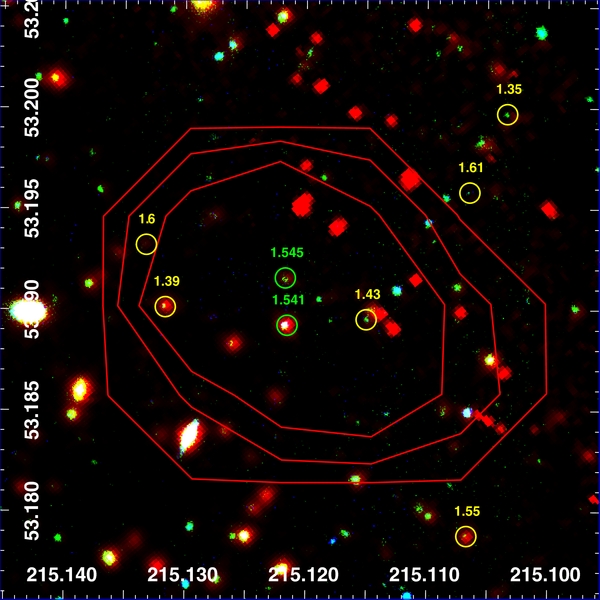
Figure 4. RGB image of the galaxy group at z = 1.54 with ID = EGSXG J1420.4+5311 using channel 2 (4.5 μm) of Spitzer/IRAC and z' and r' bands from the W3 field of CFHTLS. The contours show the X-ray emission. The green circles show spectroscopic redshifts and the yellow circles indicate galaxies located at 1.3 < zphoto < 1.7 within r200 of the group. Many of the red points are artifacts in the channel 2 image and they do not have any corresponding sources in the z' and r' bands.
Download figure:
Standard image High-resolution image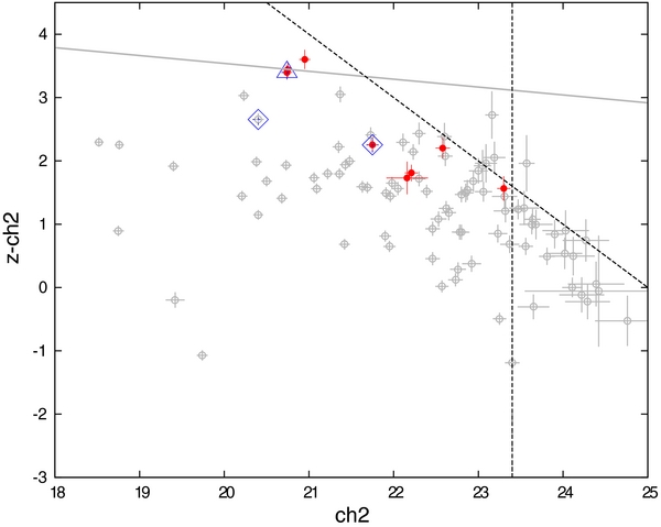
Figure 5. Color–magnitude diagram for EGSXG J1420.4+5311 based on Spitzer/IRAC and CFHTLS data. All the galaxies within r200 of the group are plotted here. The filled circles show galaxies with 1.3 < zphoto < 1.7. The diamonds and triangles indicate secure and possible spectroscopic members, respectively. The gray line shows the model's red sequence for z = 1.5. The 50% completeness for the channel 2 magnitude and z-channel 2 color are shown as vertical and slanted dashed lines, respectively.
Download figure:
Standard image High-resolution image5. SPECTROSCOPIC GROUP MEMBER GALAXIES
We search for galaxies associated with our identified X-ray sources based on their redshifts and positions. We perform this selection in different ways and explore the effects on the dynamical velocity dispersion, mass, and Lx–σ scaling relation of the groups.
First, we assume an initial velocity dispersion of 500 km s−1 for each group and calculate the redshift range for the group members from Equation (1) (Wilman et al. 2005; Connelly et al. 2012):

δ(z)max is then converted into a spatial distance using Equations (2) and (3):

with b = AspectRatio = 9.5,

where Dθ is the angular diameter distance.
Considering the center of the X-ray emission as the center of the groups, we selected group members that lie within our redshift and angular limits (Equations (4) and (5)):

and

We recompute the observed velocity dispersion of the groups, σ(v)obs, using the "gapper" estimator method which provides a more accurate measurement of velocity dispersion for small sized groups (Beers et al. 1990; Wilman et al. 2005) in comparison to the usual formula for standard deviation, σ2 = 〈v2〉 − 〈v〉2. According to the formula

where wi = i(N − i), gi = zi + 1 − zi, and N is the total number of spectroscopic members. In this way, we measure the velocity dispersion using the line of sight velocity gaps where the velocities have been sorted into ascending order. The factor 1.135 corrects for the 2σ clipping of the Gaussian velocity distribution. We then consider the r-band luminosity-weighted centroid in projected space as the center of the group and the mean redshift of the galaxy members as the group redshifts and again find the galaxy members. We repeat the entire process until we obtain a stable membership solution. For all the groups, we reach such a stable membership after two iterations. At the end, we calculated the rest-frame and intrinsic velocity dispersion according to


The intrinsic velocity dispersion, σ(v)intr, is computed by removing the effect of measurement errors of component galaxies from the rest-frame velocity dispersion, σ(v)rest (Equations (8) and (9)). We then calculated errors for our velocity dispersions using the Jackknife technique (Efron 1982). The error is [(N/(N − 1))∑(δ2i)]1/2, where  .
.
We then applied two different optical- and X-ray-based cuts for the radius used to select member galaxies. Using σ(v)intrinsic derived from member galaxies after iterating, we computed r200 for the optical cut as in Carlberg et al. (1997),
where

For the X-ray-defined radial cut, we used r200, x from the main catalog (see Section 4). We then calculated the intrinsic velocity dispersion for all groups based on Equations (6)–(9) for the members with the optical- and X-ray-based radial cuts. In Figure 6, we present a gallery of RGB images of the X-ray galaxy groups within the D3 field of CFHTLS.
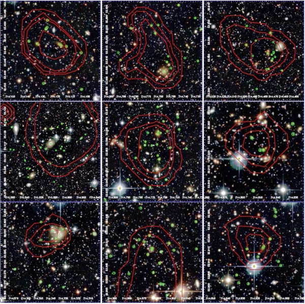
Figure 6. CFHTLS D3 RGB images of X-ray galaxy groups using g', r', and i' bands with contours indicating levels of X-ray emission (in red) and spectroscopic members of the groups inside the virial radius estimated from X-rays. From the upper left panel to the lower right panel, the group IDs are EGSXG J1416.4+5227, EGSXG J1419.0+5236, EGSXG J1417.9+5235, EGSXG J1420.0+5306, EGSXG J1419.0+5257, EGSXG J1419.4+5301, EGSXG J1417.3+5235, EGSXG J1419.8+5300, and EGSXG J1419.2+5255. The horizontal and vertical axes show the right ascension and declination, respectively.
Download figure:
Standard image High-resolution imageUsing the second method, we select the spectroscopic galaxies with positions within r200, x of the X-ray centers and find that their redshifts match to Δz1 = 0.001 × (1 + zG) and Δz2 = 0.0025 × (1 + zG), which correspond to the typical minimum and maximum velocity dispersions of the group. Table 2 shows a sample of spectroscopic galaxy members based on a 0.0025 × (1 + zG) selection. We then computed the intrinsic velocity dispersions for the member galaxies based on the X-ray virial radius and two different redshift cuts (Δz1 and Δz2).
Table 2. A Sample of Group Member Galaxies
| Group ID | R.A. | Decl. | z |
|---|---|---|---|
| EGSXG J1417.5+5238 | 214.38009 | 52.63223 | 0.7199 |
| EGSXG J1417.5+5238 | 214.36919 | 52.62006 | 0.7201 |
| EGSXG J1417.5+5238 | 214.36626 | 52.65201 | 0.7157 |
| EGSXG J1417.5+5238 | 214.41671 | 52.62889 | 0.7173 |
| EGSXG J1417.5+5238 | 214.40832 | 52.62752 | 0.7193 |
| EGSXG J1417.5+5238 | 214.40229 | 52.62471 | 0.7170 |
| EGSXG J1417.5+5238 | 214.40131 | 52.63039 | 0.7168 |
| EGSXG J1417.5+5238 | 214.39906 | 52.64248 | 0.7151 |
| EGSXG J1417.5+5238 | 214.39653 | 52.64163 | 0.7161 |
| EGSXG J1417.5+5238 | 214.39236 | 52.62690 | 0.7167 |
| EGSXG J1417.5+5238 | 214.39221 | 52.63439 | 0.7156 |
| EGSXG J1417.5+5238 | 214.38562 | 52.63828 | 0.7168 |
| EGSXG J1417.5+5238 | 214.34541 | 52.63622 | 0.7167 |
| EGSXG J1419.6+5251 | 214.90556 | 52.85547 | 0.6675 |
| EGSXG J1419.6+5251 | 214.94009 | 52.85377 | 0.6713 |
| EGSXG J1419.6+5251 | 214.92459 | 52.85621 | 0.6711 |
| EGSXG J1419.6+5251 | 214.91483 | 52.84952 | 0.6692 |
| EGSXG J1419.6+5251 | 214.90534 | 52.85083 | 0.6702 |
| EGSXG J1419.6+5251 | 214.90136 | 52.85234 | 0.6681 |
Only a portion of this table is shown here to demonstrate its form and content. A machine-readable version of the full table is available.
Download table as: DataTypeset image
In all cases, we considered galaxy groups with more than 10 members when we used the "gapper"estimator in order to have a more reliable measurement of velocity dispersion (e.g., Zabludoff & Mulchaey 1998; Girardi & Mezzetti 2001). Figure 7 shows velocity dispersions of X-ray galaxy groups derived using the "gapper"estimator method and from X-ray emission.
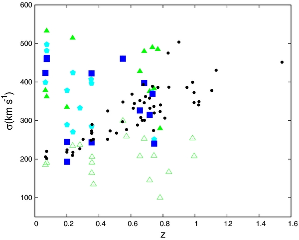
Figure 7. Velocity dispersion as a function of redshift. The black filled circles show the velocity dispersions estimated from X-ray luminosities using scaling relations for all the groups. The filled and empty triangles show the velocity dispersions for the groups with Δz2 and Δz1, respectively. The pentagons show the velocity dispersions for the groups with an optically determined radial cut after iterations and the squares show the velocity dispersions for the groups with an X-ray radius cut after iterations.
Download figure:
Standard image High-resolution image5.1. The Relation between X-Ray Luminosity and Dynamical Velocity Dispersion
Figures 8 and 9 show the X-ray luminosity versus velocity dispersion for different methods. These plots include all the galaxy groups with Flag = 1 and 2. We also plot the Lx–σ relation (dashed line) expected from scaling relations obtained for a sample of groups with similar luminosities in the 0 < z < 1 redshift range in COSMOS (Leauthaud et al. 2010).
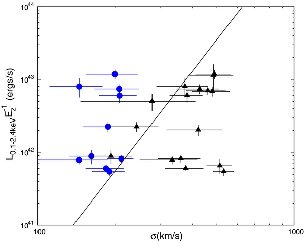
Figure 8. LX–σ relation for X-ray groups. The blue circles and the black triangles correspond to groups whose members match Δz1 and Δz2, respectively. The solid line shows our expectation for the LX–σ relation derived from scaling relations.
Download figure:
Standard image High-resolution image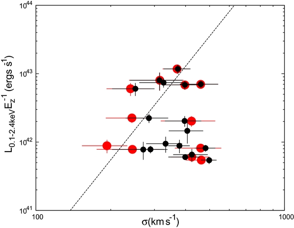
Figure 9. LX–σ relation for X-ray groups whose members lie within a dynamically based virial radius (black circles) and X-ray-based virial radius (red circles).
Download figure:
Standard image High-resolution imageVelocity dispersions can be biased toward higher values for low-mass systems when we select members based on large Δz, as we may include outliers in our calculation and conversely can be biased toward lower values for high-mass systems if we select member galaxies within low Δz along the line of sight as we are then ignoring some parts of the group (Figure 8). Furthermore, tracking the groups while we use different Δz to choose member galaxies reveals an average systematic error of ∼190 km s−1.
Figure 9 shows the Lx–σ relation for galaxy groups whose members are selected based on two different radial cuts. It is obvious from Figure 9 that different radial cuts can cause a change in the scatter of the Lx–σ relation but, in the case of high-mass systems, there is no apparent change in the scatter of this relation. In addition, low X-ray luminosity systems show significant deviations from the scaling relation in both X-ray and optically based radial cuts.
We look at the quality flags, dynamical complexity, and the X-ray compactness in comparison to the virial radius for the groups in order to study the group properties and their effects on the relation.
As we expect, Figures 10 and 11 illustrate that galaxy groups with Flag = 2 have significant deviations from the relation compared to galaxy groups with Flag = 1 (similar to what Connelly et al. 2012 found for the intermediate-redshift X-ray-selected groups).
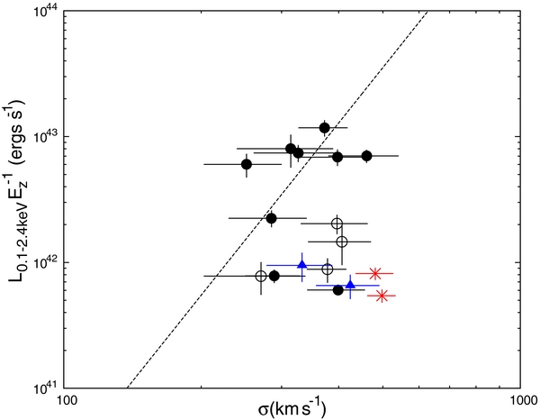
Figure 10. LX–σ relation for X-ray groups whose members lie within a dynamically based virial radius. The red stars show groups that have substructure detected by the DS test, the blue triangles are the compact X-ray systems, and the open circles show the groups with Flag = 2. The solid line shows our expected LX–σ relation derived from scaling relations.
Download figure:
Standard image High-resolution image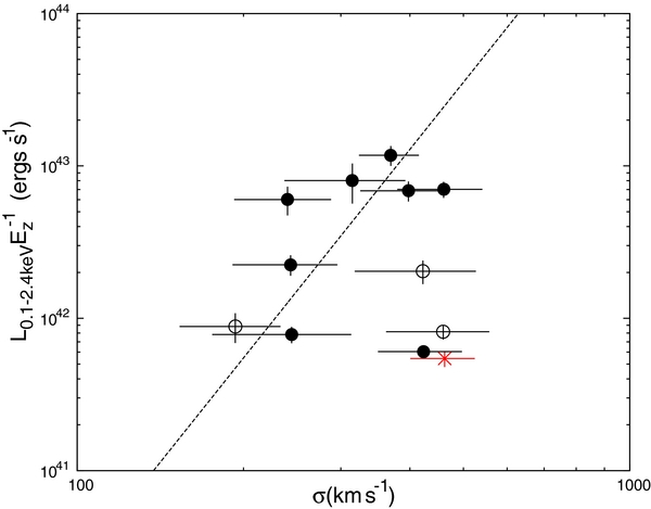
Figure 11. LX–σ relation for X-ray groups given a radial cut based on X-rays. The red stars show groups that have substructure detected by the DS test, the blue triangles are the compact X-ray systems, and the open circles show the groups with Flag = 2. The solid line shows our expectation for the LX–σ relation derived from scaling relations.
Download figure:
Standard image High-resolution imageTo search for substructure in our groups, we apply the Dressler–Shectman (DS; Dressler & Shectman 1988) test. We use the DS test as in Hou et al. (2012) who implement it for group sized systems. In brief, we consider each individual galaxy in the group plus the Nnn nearest members to it with  and calculate the mean velocity and velocity dispersion for them (
 ). We then compute the deviations for each galaxy from the mean velocity (
 ) and velocity dispersion (σ) of the whole group with nmem galaxies:
where 1 ⩽ i ⩽ nmembers. Then Δ statistics are computed using
To identify substructure, we use a probability (P-values) threshold for the DS test, and run 10,000 Monte Carlo simulations for each group. In each Monte Carlo run, the observed velocities are randomly shuffled and reassigned to member positions and Δshuffled is computed. The probabilities are given by

where nshuffle is the number of the Monte Carlo simulations which in our case is 10,000. A system is then considered to have significant substructure with a 99% confidence level when P < 0.01. In total, we found 2 galaxy groups of 17 in the optically based radial cut groups and 1 group of 12 in the X-ray-based radial cut galaxy groups with significant substructure, which are marked with stars in Figures 10 and 11.
Figure 12 shows the optical images for three galaxy groups that have the largest deviations from the scaling relation in Figure 10. All of them have Flag = 1 and substructure is not detected using the DS test. The two images on the left in Figure 12 have less than 10 members given an X-ray-based virial radius cut and are not included in Figure 11. We compared the extension of the X-ray emission to the virial radius extracted from the X-ray and optical velocity dispersion for galaxy groups. As Figure 13 shows, there is a population of group galaxies for which the fraction of the extension of X-rays to the virial radius is less than 20% in the optically based radial cut and less than 15% in the X-ray-based radial cut. These populations are dominated by some galaxy groups with Flag = 2 and two galaxy groups on the left in Figure 12 with an overluminous galaxy close to the X-ray center.

Figure 12. CFHTLS D3 RGB images of X-ray galaxy groups using g', r', and i' bands with contours indicating levels of X-ray emission (in red) and spectroscopic members (in green). The group IDs from left to right are EGSXG J1418.3+5227, EGSXG J1417.3+5235, and EGSXG J1417.7+5241.
Download figure:
Standard image High-resolution image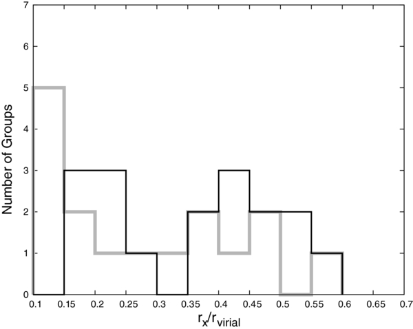
Figure 13. Fraction of X-ray extent to virial radius for an X-ray-based virial radius (black line) and an optically based virial radius (gray line).
Download figure:
Standard image High-resolution imageWe explored the Lx–σ relation in more detail for the three groups with large deviations from the scaling relation (Figure 12). EGSXG J1418.3+5227 with Lx = 1.08 × 1042 erg s−1 has Δm12 = 2 where Δm12 is the r-band magnitude difference between the first and the second brightest galaxy located in half of the virial radius of the group. These conditions result in the classification of this group as a fossil galaxy group candidate (Jones et al. 2003). As fossil galaxy groups are believed to be the final result of galaxy merging in normal groups, we expect a sufficiently deep potential well and high X-ray luminosity for these systems (Ponman et al. 1994; Jones et al. 2000b). As a consequence, we expected these fossil groups to be more X-ray luminous than normal groups at a given velocity dispersion (Khosroshahi et al. 2007), but instead we found the opposite. Moreover, Osmond & Ponman (2004) applied a radius of 60 kpc as a threshold for detectable X-ray emission in order to separate galactic halos from group-scale halos using different studies of bright isolated galaxies (O'Sullivan et al. 2003; O'Sullivan & Ponman 2004). The radius of detectable X-ray emission (at which the group emission fell to the background level) for EGSXG J1418.3+5227 is greater than this threshold and about 95 kpc. However, the nature of this X-ray-extended source with such unexpectedly low X-ray emission compared to the velocity dispersion is still a matter of interest.
In the cases of EGSXG J1417.3+5235 and EGSXG J1417.7+5241, both having large numbers of spectroscopic member galaxies, the estimation of velocity dispersion cannot be the main uncertainty. EGSXG J1417.3+5235 satisfies all three criteria (population, isolation, and compactness) for a compact group (Hickson 1982). As a compactness criterion, Hickson (1982) establishes that the sum of the member galaxies' magnitude averaged over the smallest circle containing the cores of the most luminous galaxies in a compact group should be less than 26 in the POSS-I E band, μE < 26 mag arcsec−2. He uses the POSS-I E band for the cut on the surface brightness of his local groups, which roughly corresponds to the r band (e.g., Díaz-Giménez et al. 2012). As all of his compact groups are in the local universe, we should apply the k-correction to the r-band magnitude of the member galaxies of EGSXG J1417.3+5235 at z = 0.236. All galaxies that we use for computing surface brightness are on the red sequence, therefore, we calculate the k-correction to the r-band magnitude using the stellar population model of Maraston et al. (2009) for red galaxies. Using the k-corrected magnitudes, this group satisfies the compactness criterion. It also has a high concentration of X-ray emission (Figure 13), while having low mass, leading to a steep X-ray profile. However, Helsdon & Ponman (2000) find that the loose and compact local groups lie in a similar position on the LX–σ relation. Figure 14 shows the histogram of velocity distribution of the member galaxies and the expected Gaussian distribution from the scaling relations for EGSXG J1417.3+5235.

Figure 14. Solid line shows the histogram of velocity distribution of EGSXG J1417.3+5235. The dashed Gaussian curve is the expected velocity distribution from the scaling relation for this group.
Download figure:
Standard image High-resolution imageExcluding these three groups, the Flag = 2 groups, and also the group with substructures, the Lx–σ relation of our sample is consistent with the Lx–σ relation expected from scaling relations obtained from COSMOS (Leauthaud et al. 2010).
5.2. X-Ray Mass versus Dynamical Mass
We also estimated dynamical mass for the galaxy groups using r200 (Equation (10)) and the intrinsic velocity dispersion as in Balogh et al. (2006) and Carlberg et al. (1999):

As we expected from the Lx–σ relation of the groups (Figures 10 and 11), we find much better agreement between dynamical mass and X-ray mass for high-mass systems (Figure 15). For low-mass systems with a low-quality flag (Flag = 2) and substructure, the disagreement between these two masses is more substantial. In addition, the errors on dynamical mass are increased in the X-ray-based r200, as the groups have less members in this case when compared to that of an optically based r200.
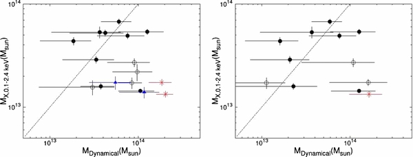
Figure 15. X-ray mass vs. dynamical mass for the X-ray galaxy groups. The left panel shows the galaxy groups with members selected within the velocity-dispersion-based r200. The right panel shows galaxy groups with members within the X-ray-based r200. The red stars show groups that have substructure detected by the DS test, the blue triangles are the compact X-ray systems, and the open circles show the groups with Flag = 2. The dashed line is the one-to-one relation.
Download figure:
Standard image High-resolution image6. COMPARISON TO OPTICAL GROUPS
The optical group catalog is derived from the DEEP2 DR4 data set using the VDM group finder (Gerke et al. 2012) and includes groups in all DEEP2 fields. It yields 1165 groups with more than two observed members in the EGS field. We look at the distribution of redshifts for our X-ray and optically selected groups, and in Figure 16 we show the normalized distribution of redshifts for both samples. The X-ray groups are preferentially found at z > 0.6, compared to the optical groups, but, in general, the two distributions are similar.
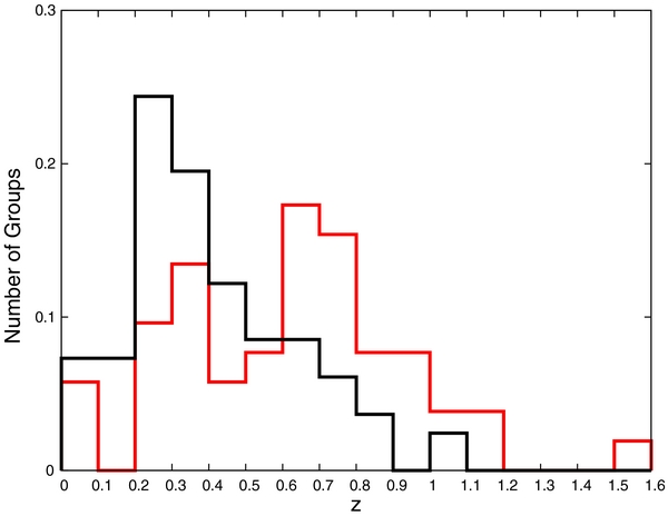
Figure 16. Normalized distribution of redshift for X-ray galaxy groups (in red) and optical galaxy groups (in black) inside our flux detection limits in the EGS.
Download figure:
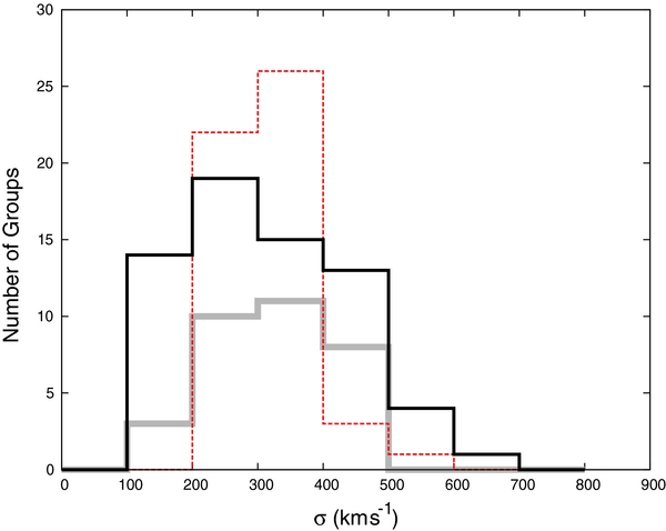
Standard image High-resolution imageWe also compared velocity dispersions of both samples. In order to have a reliable comparison we take into account only optical groups with our X-ray detection limit. Figure 17 shows the distribution of rest-frame velocity dispersion for galaxy groups with more than five members. For X-ray galaxy groups, we plot both the velocity dispersions derived from X-ray properties and the gapper estimator method. The velocity dispersion of the optical groups is the observed velocity dispersion derived using the gapper algorithm. We converted them to rest-frame velocity using Equation (7) for comparison.
Figure 17. Distribution of velocity dispersion for optical and X-ray galaxy groups. The black line shows the distributions of velocity dispersion of the optical VDM groups. The dashed red and thick gray lines correspond to the distributions of velocity dispersion estimated from X-rays and the dynamical velocity dispersion for X-ray groups.
Download figure:
Standard image High-resolution image
We searched for the high-velocity tail of the distribution of the optical group velocity dispersion in the X-ray data. This high-velocity tail arises from galaxy groups with less than 10 members, which are actually part of a bigger group or on the edge of the X-ray coverage of EGS. Ignoring this tail, in general, these distributions are also similar.
7. SUMMARY AND DISCUSSION
We have searched for X-ray extended sources in AEGIS. We identified X-ray galaxy groups corresponding to extended X-ray emissions and presented the galaxy groups catalog. The catalog reaches a flux of 10−15 erg s−1 cm−2 with 52 systems detected by Chandra. Previously Chandra catalogs at such depths contain about half a dozen objects per field (Giacconi et al. 2002; Bauer et al. 2002). The DEEP2 and DEEP3 redshift surveys, which provide the most complete sample at intermediate redshift and the largest accurate data sets at z ∼ 1, combined with deep X-ray imaging from Chandra in the EGS field, bring a deep study of galaxy groups to a new level. Spectroscopic member galaxies are selected by applying different cuts: two X-ray-based and optically based virial radii and two cuts along the line of sight. We examined the Lx–σ relation for each cut and discussed their effects on the relation. We explored substructure in the groups by applying the DS test and discussed its effect on the overestimation of velocity dispersion. We also looked at the compactness of the X-ray emission of the groups and its effect on the scaling relation. A comparison between the dynamical mass and X-ray mass of the groups is also done. Finally, X-ray galaxy groups are compared with optical galaxy groups which are identified from VDM groups. Our results show the following. (1) Our detection of a high-z group illustrates that megasecond Chandra exposures are required for detecting such objects in the volume of deep fields. Smaller exposures, such as in Pierre et al. (2012), only yields a marginal detection. (2) For a sample of groups with a wide range of X-ray luminosities, the choice of a constant Δz for member selection can cause a large scatter in the Lx–σ relation. (3) The choice of X-ray-based virial radius or optically based virial radius does not have a significant effect on the scatter around the Lx–σ relation for groups with high X-ray luminosities. (4) Substructure in groups can inflate velocity dispersion as outliers are also included in galaxies with dynamical complexity. (5) We find a compact group at z = 0.24 with a concentrated X-ray emission with high velocity dispersion in comparison to X-ray luminosity. (6) X-ray galaxy groups and optical galaxy groups from VDM are nearly similar in both redshift and velocity dispersion distributions.
We thank David Wilman, Annie Hou, and Antonis Georgakakis for helpful discussions about the dynamical properties and AGN contamination of X-ray groups. We also thank Felicia Ziparo and Steve Willner for useful comments on the manuscript. M.T. acknowledges support from the World Premier International Research Center Initiative (WPI Initiative), MEXT, Japan and from KAKENHI No. 23740144. This work was also supported in part by National Science Foundation grants AST 00-71198, 05-07483, and 08-08133 to the University of California, Santa Cruz; AST 00-71048, 05-07428, and 08-07630 to the University of California, Berkeley; and AST 08-06732 to the University of Pittsburgh. This project has been supported by the DLR grant 50OR1013 to M.P.E.
Footnotes
- 20
- 21
Based on observations obtained with MegaPrime/MegaCam, a joint project of CFHT and CEA/DAPNIA, at the Canada–France–Hawaii Telescope (CFHT), which is operated by the National Research Council (NRC) of Canada, the Institut National des Science de l'Univers of the Centre National de la Recherche Scientifique (CNRS) of France, and the University of Hawaii. This work is based in part on data products produced at TERAPIX and the Canadian Astronomy Data Centre as part of the Canada–France–Hawaii Telescope Legacy Survey, a collaborative project of NRC and CNRS.
- 22
- 23
Funding for the SDSS and SDSS-II has been provided by the Alfred P. Sloan Foundation, the Participating Institutions, the National Science Foundation, the U.S. Department of Energy, the National Aeronautics and Space Administration, the Japanese Monbukagakusho, the Max Planck Society, and the Higher Education Funding Council for England. The SDSS Web site is http://www.sdss.org/.