


ABSTRACT
We present a new analytic approach to the disk–planet interaction that is especially useful for planets with eccentricity larger than the disk aspect ratio. We make use of the dynamical friction formula to calculate the force exerted on the planet by the disk, and the force is averaged over the period of the planet. The resulting migration and eccentricity damping timescale agree very well with previous works in which the planet eccentricity is moderately larger than the disk aspect ratio. The advantage of this approach is that it is possible to apply this formulation to arbitrary large eccentricity. We have found that the timescale of the orbital evolution depends largely on the adopted disk model in the case of highly eccentric planets. We discuss the possible implication of our results for the theory of planet formation.
Export citation and abstract BibTeX RIS
1. INTRODUCTION
The gravitational interaction between a planet and a protoplanetary disk is one of the main topics of the theory of planet formation. A low-mass planet embedded in a protoplanetary disk interacts with the disk by the gravitational force, and its orbital elements change as a result of this interaction. The change of the semimajor axis of the planet is called (type I) orbital migration. It has recently been noted that the direction of migration is sensitive to the disk model if the planet is in a circular orbit (e.g., Paardekooper & Mellema 2006; Paardekooper et al. 2010a, 2010b).
Observations of extrasolar planets have revealed that there are a number of planets with high eccentricity, and the median eccentricity is ∼0.3 (Udry & Santos 2007). One interesting question here is whether it is possible to have an eccentric planet in a circular disk. Recent numerical simulations (Cresswell et al. 2007; Bitsch & Kley 2010) show that the eccentricity always damps. It is reported that the eccentricity damping and the migration timescales do not strongly depend on the physical state of the gas (e.g., radiative or locally isothermal) for a planet with high eccentricity, and the timescale becomes longer if the eccentricity becomes larger.
Linear analysis of the interaction between a disk and a planet has been done by a number of authors (e.g., Goldreich & Tremaine 1980; Artymowicz 1993; Tanaka & Ward 2004) for a planet with low eccentricity. In particular, Papaloizou & Larwood (2000) obtained the eccentricity damping timescale and migration timescale for a planet with e ≳ h, where e is the eccentricity of the planet and h is the disk aspect ratio (h = H/r, where H is the disk scale height and r is the disk radius), but their approach is restricted to e ≪ 1. Tanaka & Ward (2004) performed three-dimensional modified local linear analyses2 to calculate the gravitational interaction between a disk and a planet in an eccentric orbit. They calculated the density perturbation at every location of the orbit; therefore, it is possible to calculate the instantaneous force acting on the planet at every position on the orbit. The instantaneous force acting on the planet is then averaged over the orbital period to obtain the timescales of the orbital evolution. We note that since they use the (modified) local approximations, their results can be applied to the case in which the eccentricity of the planet is small compared to the disk aspect ratio.
In this paper, we present an analytical model for the interaction between a low-mass planet in an eccentric orbit and a disk. In contrast to the previous approach in which one uses Fourier decomposition and calculates the contributions from Lindblad and corotation resonances (e.g., Papaloizou & Larwood 2000), we make use of the dynamical friction formula to estimate the force acting on the planet at every location on the orbit. The force is then averaged over the orbital period to obtain the evolution timescales of the orbital parameters. Using this "real-space" model, it is also possible to obtain more intuitive pictures of the disk–planet interaction. We note that most of the highly eccentric planets detected so far are gas giants, but we consider a low-mass planet in this paper to make the problem simpler. Our analytic approach would reveal an underlying physical mechanism of the planet–disk interaction, which we believe would be useful in the investigation of high-mass planets as well. We also note that, in the course of the formation processes of the planets, it is important to understand the evolution of the orbital parameters of a low-mass protoplanet or the core of the gas giants. In this case, our approach based on linear perturbation analyses may be directly applicable.
Our approach is similar to that of Tanaka & Ward (2004) in the sense that we calculate the force acting on the planet at every instance of the orbit. The major difference, however, is that we use a very simple model for the force acting on the planet. As we shall show later in this paper, our approach is especially useful for the case with eccentricity larger than the disk aspect ratio, and we expect that it is possible to use our model for a planet with an arbitrary large eccentricity. Therefore, we are in the parameter space that is complementary to Tanaka & Ward (2004). However, it is noted that the use of a simple model is also the limitation of our approach, and we shall discuss the applicability of the model toward the end of the paper.
The dynamical friction in a gaseous medium itself is also an interesting topic investigated by a number of authors. Rephaeli & Salpeter (1980) investigated the stationary pattern around a gravitating object in a homogeneous medium using a linear perturbation analysis and concluded that the dynamical friction force vanishes if the particle's speed is subsonic, while the dynamical friction force varies as v−2 in the supersonic case, where v is the speed of the particle. The result in the supersonic case is in agreement with the case of the collisionless system (Chandrasekhar 1943).
The conclusion of zero dynamical friction force seems rather counterintuitive since the drag force may experience a sudden drop when the particle's speed transitions from supersonic to subsonic. This apparent contradiction is resolved by Ostriker (1999) who performed the time-dependent analysis. She showed that the dynamical friction force depends linearly on the speed of the particle when it moves at a subsonic velocity, while the force depends on v−2 for the supersonic case. The results of Ostriker (1999) obtained by linear perturbation analyses are in good agreement with nonlinear numerical simulations (Sánchez-Salcedo & Brandenburg 1999).
After these works, there are a number of works on this topic with different configurations of the problem (e.g., Kim et al. 2005; Kim & Kim 2007, 2009), but it seems there has not been a work considering a slab geometry, which can be applied to the problem of the disk–planet interaction.
In this paper, we first perform a linear perturbation analysis and derive an analytical formula for the dynamical friction force exerted on a particle embedded in a homogeneous slab of gas. We then apply the formula to the problem of the disk–planet interaction. We consider the case in which the planet is in an eccentric orbit. Although the gas flow in a protoplanetary disk is not homogeneous, we show that it is actually possible to obtain reasonable results if the planet is in an eccentric orbit. We note that the results of the dynamical friction force may have different astrophysical applications from the problem of the disk–planet interaction.
This paper is constructed as follows. In Section 2, we derive the dynamical friction force exerted on a point particle embedded in a homogeneous gas slab. In Section 3, we apply the dynamical friction formula obtained in Section 2 to the problem of the disk–planet interaction. We discuss some possible applications to the planet formation theory in Section 4 and present a summary in Section 5.
2. DYNAMICAL FRICTION IN A GASEOUS SLAB
In this section, we consider the dynamical interaction between a point particle and the homogeneous, viscous gaseous slab in which the particle is embedded. We show that it is possible to obtain a dynamical friction formula whose behavior is similar to that of Ostriker (1999) in this setup, although there is additional dependence on the viscosity as well as the Mach number of the particle. We also show that in the limit of a high Mach number, the resulting formula does not depend on the viscosity.
2.1. Basic Setup
We consider a homogeneous gaseous slab with surface density Σ0. We take the Cartesian coordinate system (x, y) in the plane of the slab and consider a point particle with mass M traveling in the y-direction at a constant speed v0. The basic equations we consider are the (vertically integrated) hydrodynamic equations with a simplified prescription of viscosity,


where Σ is the surface density,  is the velocity, P is the (vertically integrated) pressure, ν is the viscous coefficient, and ψ is the gravitational potential of the particle. We use a simple form of viscosity in order to keep the problem simple and tractable. We use a simple, isothermal equation of state

where c is the sound speed. We consider an inertial coordinate system in which the particle is always at the origin so the background flow velocity is given by  . For the gravitational potential, we make use of the form that is commonly incorporated in the investigation of the disk–planet interaction in two-dimensional analyses,

where  is the softening length, which is a sizable fraction of the thickness of the slab in order to mimic the three-dimensional effects.
This form of the gravitational potential (4) is the model for the vertically averaged gravitational potential; therefore, the softening length should be of the order of the vertical scale length of the disk. It is to be noted that, with this form of the potential, the gravitational potential close to the point mass (typically, the distance closer than ) is underestimated. If the vertical averaging is taken, the potential close to the mass behaves as ∝log r, where r is the distance from the point mass, in contrast to Equation (4), which behaves as a constant for r ≲ .
However, as we shall show later, the main contribution to the dynamical friction force comes from the region r ∼ , and the contribution from the region r < would affect the results by only some factor. It is also noted that the dependence of the force on the physical parameters can be captured with the form of the potential given by Equation (4). Therefore, we use this form of the potential as a model for the vertically averaged potential in this paper. The outcome of this approximation will be discussed in detail later in this section. We also note that this form of the potential is widely used in the numerical calculations of the disk–planet interaction. One benefit of using the simple form of the gravitational potential given by Equation (4) is that it is possible to obtain an analytic expression for the dynamical friction.
2.2. Linear Perturbation Analysis
We now perform the linear perturbation analysis to calculate the surface density perturbation induced by the particle's gravity. We use the subscript zero to indicate the background quantities, and we denote all the perturbed quantities by δ, e.g., surface density is given by Σ = Σ0 + δΣ. We retain the terms up to the first order of the perturbation. Equations (1) and (2) now become


From these equations, we derive a single second-order differential equation for the surface density perturbation,

where we have defined α ≡ δΣ/Σ0, and ∇2 = (∂/∂x)2 + (∂/∂y)2 is the Laplacian.
We now consider a steady state where ∂/∂t = 0. In Ostriker (1999), it is pointed out that it is necessary to perform a time-dependent analysis in order to correctly obtain the dynamical friction force, especially when the particle's velocity is subsonic. This is because the contribution to the force coming from a place very far from the particle is not negligible. However, as we shall show below, the analysis assuming the steady state is adequate in the slab geometry we consider in this section since the perturbation induced at a distant place from the particle does not contribute to the force.
In Appendix A, we explicitly show that the force coming from the time-dependent terms falls as t−1. Here, we briefly show this by the order-of-magnitude estimate. If we consider the place far from the particle, the gravitational potential is given by

where r is the distance from the particle. We expect that this gravitational energy is of the same order of magnitude as the perturbed thermal energy of the gas. In the three-dimensional analysis, we therefore expect that

where ρ is the gas density. In the slab geometry, we expect that

where Σ is the surface density. In the three-dimensional analysis, the force δF acting on the particle from the gas shell at the distance r with the width δr is

The force from the shell decays only with r−1. Therefore, when summed over all the shells, the contribution from the distant shell is not negligible.3 In the case of two-dimensional slab geometry, on the other hand, the force from the ring at distance r with width δr is

The force from the distant ring decays as r−2; therefore, the contribution from the distant ring does not account for the total force when summed over all the rings. We note here that the contribution to the dynamical friction force far from the planet decays as r−1 if we integrate all the rings. This explains why the force decays as t−1 in the subsonic case if we consider the slab geometry. The rings that contribute to the dynamical friction force reside at r ∼ ct, as pointed out by Ostriker (1999).
In this paper, we shall show in detail the derivation of the dynamical friction force exerted on the particle embedded in a gaseous slab using the two-dimensional approximation. Before going on to the details, we show that the dependences of the force on the physical parameters of the gas can be derived through the two-dimensional approximation.
In the realistic case of the gaseous slab with the thickness of Lz(∼ ), the interaction between the gas and the particle can be well approximated by the two-dimensional analysis for the scales larger than Lz (far region). Inside this region (near region), the interaction should be calculated in three dimensions. Integrating Equation (12) between the minimum cutoff scale rmin and γLz (γ is a factor of the order of unity), the contribution to the dynamical friction force from the near region, FN, is given by

The contribution to the force from the far region, FF, is given by integrating Equation (13) from γLz to infinity and

where we have used Σ ∼ ρLz. The integral from the far region does not diverge at r = ∞ since there is not enough mass to contribute to the force in the slab geometry in the far region, in contrast to the case of the homogeneous three-dimensional distribution of the gas. It should be noted that the dependences of the force on physical parameters in FF and FN are the same except for the logarithmic factor, which only introduces very weak dependences on Lz and rmin. By choosing the appropriate value of γ, it is possible to have an expression that would reproduce the results of three-dimensional calculations from two-dimensional calculations. Therefore, we expect that the two-dimensional analyses can be used to understand the fundamental aspects of the dynamical friction force. More detailed discussions on the two-dimensional approximation in relation to the application to the disk–planet interaction can be found in Section 2.5.
We now derive the steady-state solution of Equation (8). We make use of the Fourier transform to solve the equations, but our goal is to derive the expression of the force exerted on the particle, which is, of course, the quantity in the real space. For any perturbed quantity f (x, y), we define the Fourier transform by

and the inverse transform is

The steady state of surface density perturbation can be derived from Equation (8) in the Fourier space as

where k2 = k2x + ky2.
If we know the profile of the perturbed surface density, the dynamical friction force exerted on the particle is calculated by

We note that the x-component of the force is zero because of the symmetry. From the solution in the Fourier space, the dynamical friction force is given by

where the Fourier transform of the gravitational potential  is given by

We comment that in Equation (20), we integrate the contribution to the force coming from all over the space, including the region close to the particle. The contribution to the force coming from the near region is effectively cut off due to the softening. This is actually a reasonable treatment, given the uncertainty of the softening length , and it is possible to derive the dependences of the force on physical parameters. See Section 2.5 for more detailed discussions.
We calculate the dynamical friction force using Equations (18) and (20). By changing the integration variables first from (kx, ky) to (k, θ) via

and

and then from k to u = νv0k/c2, we can rewrite the integral as

where M0 ≡ v0/c is the Mach number of the background flow and Γ ≡ 2c/M0ν. The function Iθ(p, q) that appears in the integral is given by

It is actually possible to perform the integration involved in Iθ(p, q) analytically. The explicit form of this is found in Appendix B.
2.3. Expressions in Some Limits
It is now possible to perform the integral (24) numerically to obtain the dynamical friction force in a gaseous slab if we give two dimensionless parameters M0 and Γ. However, for a moment, we look at some limits to obtain analytic expressions in order to investigate how the dynamical friction force depends on these parameters.
2.3.1. Subsonic Limit
We first look at the subsonic case where M0 ≪ 1. In this case, we approximate 1 − M20sin θ ∼ 1 so the integral (25) becomes

Therefore, in the limit of u → 0, Iθ(M20, u2) ∼ π while in the limit of u → ∞, Iθ(M20, u2) ∼ 2π/u2. Connecting these two limits, we approximate the integral by

The dynamical friction force is obtained from Equation (24). It is possible to perform the integral analytically and we have

where Ei(x) is the exponential integral defined by

In the limit of subsonic perturbation, we expect that Γ ≫ 1. We then obtain

The dynamical friction force is proportional to the speed of the particle and also the viscosity. In the case of an inviscid, steady state with a subsonic particle embedded in the gaseous slab, the dynamical friction force vanishes as indicated by the time-dependent analysis shown in Appendix A.
2.3.2. Supersonic Limit
We now consider the supersonic limit where M0 ≫ 1. We first consider the behavior of the integral Iθ(M20, u2) separately in the two limits, u ≪ M20 and u ≫ M20.
In the case of u ≪ M20, the dominant contribution to the integral comes from θ ∼ θ0, where θ0 is given by

Approximating sin θ = sin (θ0 + δθ) to the first order of δθ,

the integral can be approximated by

where the factor of four comes from the fact that there are four positions within 0 < θ < 2π where sin 2θ equals 1/M20, and the range of integration is extended from −∞ to ∞. The integrand of Equation (33) is the Lorentzian function with width ∼u/M20. The condition where this width must be very small compared to the unity (or more exactly 2π, in order to justify the extension of the range of the integration) leads to the condition u ≪ M20. Using the formula

we obtain
In the case of u ≫ M20, the width of the Lorentzian is too wide to extend the integration range from (0, 2π) to (− ∞, ∞). In this case, we expect that u2sin 2θ ≫ (1 − M20sin 2θ)2 is satisfied in the most part of θ. We also approximate 1 − M20sin 2θ ∼ −M02sin 2θ so we can rewrite the integral as

Using the formula

we obtain

where we have used the condition u ≫ M20. In summary, in the supersonic limit, the integral (25) can be approximated by
We can now perform the integral (24) to give the dynamical friction force. The result is
In the supersonic limit, we expect that ΓM20 ≫ 1. In this case the expression simplifies to

As expected, we obtain that the force is proportional to v−20.
We note that the dynamical friction force is independent of the viscosity in the supersonic limit. This indicates that the dynamical friction force in the supersonic limit is insensitive to the dissipation process. We conjecture that the dynamical friction force is insensitive to the physical state of the slab (whether the slab is isothermal or radiative) in the case of the supersonic motion. A similar situation happens in the discussion of the Lindblad torque exerted on a planet embedded in a disk (Meyer-Vernet & Sicardy 1987).
2.4. Dynamical Friction Force
We now come to the point where we consider all the values of M0. We integrate Equation (24) numerically to find the dependence of the dynamical friction force on the physical parameters. As we have seen in the above analytic discussions, there are two dimensionless parameters, Γ and M0, in the problem at hand. In this section, we use the "Reynolds number," Re, defined by

instead of Γ, since the parameter Γ contains both the Mach number and the viscous coefficient.
Figure 1 shows the dependence of the dynamical friction force normalized by Σ0(GM)2/c2 as a function of the Mach number and the Reynolds number. In the subsonic regime, we see the expected behavior from Equation (30) where dynamical friction force decreases as we decrease the Mach number and viscosity. For the supersonic case, we also see the behavior expected from Equation (41) where the force decreases as we increase the velocity but the force only weakly depends on the values of viscosity.
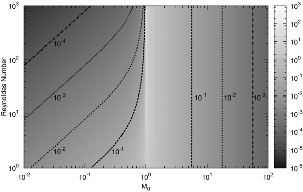
Figure 1. Dynamical friction force obtained by the numerical integration of Equation (24). The results are normalized by Σ0(GM)2/c2. The horizontal axis shows the Mach number and the vertical axis shows the Reynolds number (defined in the main text).
Download figure:
Standard image High-resolution imageFigure 2 shows the dependence of the dynamical friction force on the Mach number in the case of Re = 100, and we also show the formulae in the subsonic and supersonic limits, Equations (30) and (41). These limiting formulae well describe the behaviors of the dynamical friction force. Equation (41) is actually a good approximation of the dynamical friction force even in the case of M0 ∼ 2.
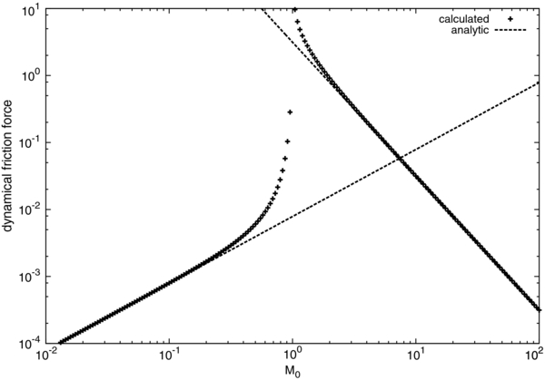
Figure 2. Dynamical friction force for Re = 100. The results of the numerical integration of Equation (24) are shown by plus symbols, and the analytic formulae in the limit of supersonic and subsonic cases, which are given by Equations (30) and (41), respectively, are shown by dashed lines.
Download figure:
Standard image High-resolution imageWe briefly comment on the divergence at M0 = 1. In Figures 1 and 2, we see that the dynamical friction force diverges at M0 = 1. This divergence comes from the matching between the background velocity and the sound speed, and was already seen in the previous linear analyses by Ostriker (1999). It is not possible to avoid this divergence by the effect of viscosity. We consider that nonlinear effects are important here.
2.5. Validity of Two-Dimensional Approximation
We have derived the dynamical friction force exerted on a particle embedded in a homogeneous gas slab using the two-dimensional approximation. We now discuss the validity of this approximation in the subsonic and supersonic cases.
As we have discussed before, the two-dimensional treatment is based on the averaging of the equations in the vertical direction, and the phenomena that occur on the scales larger than the vertical averaging scale can be well approximated by the two-dimensional calculations. In our model, the vertical averaging scale is given by , which is the softening scale of the gravitational potential in Equation (4).
In the subsonic case, the dominant contribution to the integral (24) comes from  , which is
  . This indicates that in the subsonic case, the perturbation with the scale comparable to the gravitational softening length becomes important in determining the dynamical friction force. Therefore, it is indicated that the full three-dimensional treatment may be necessary to have more quantitative results.
In the case of the supersonic motion, let us consider the case in which ΓM20 = 2v0/ν ≫ 1 for simplicity. In this case, the integral (24) for the dynamical friction force is approximated by

therefore, all the scales satisfying Γu ∼ k ≲ 1 contribute to the force. In other words, this includes all the scales from the large scale (small k), where we expect that the two-dimensional approximation is valid, down to the cutoff scale contribute to the force. Since the dependence of the cutoff scale is also present in the case of the supersonic motion, rigorous three-dimensional treatment is necessary to give more quantitative expressions of the dynamical friction force.
However, we expect that it is possible to capture the dependences on physical parameters even in the two-dimensional approximation. In the beginning of Section 2.2, we have estimated the order of the magnitude of the dynamical friction force in Equations (12) and (13), and the contribution from the near region (14) and that from the far region (15) differ by only a logarithmic factor log (Lz/rmin). The dynamical friction force derived in this paper corresponds to the contribution from the far region. The lack of the logarithmic factor is due to the fact that the potential is smoothed in the region r ≲ (see also the discussion after Equation (4)). We note the similarity of the expressions derived by the simple order-of-magnitude estimate (15) and more rigorous calculations (41).
In order to estimate the contribution from the near region, it is necessary to determine the appropriate value of rmin. However, it is not straightforward; there are several publications on this using the nonlinear calculations (e.g., Sánchez-Salcedo & Brandenburg 1999; Kim & Kim 2009). Let us consider, for a moment, the case of the planet embedded in a protoplanetary disk. The naive estimate of rmin is the radius of the planet, and in the case of an Earth-mass planet, it is of the order of 104 km. If we use the typical disk scale height H ∼ 0.05 AU, the value of log (H/rmin) amounts to ∼7. Recent nonlinear calculations (Kim & Kim 2009) suggest that the deviation from the linear value may be smaller due to the shock formation. If we use rmin ∼ GM/v2, which is the typical scale of the distance between the particle and the shock in supersonic motion (e.g., Kim & Kim 2009), instead of the planet radius for rmin, the logarithmic factor is ∼3–6 for an Earth-mass body. We shall present further discussions on the nonlinear effects on dynamical friction at the end of Section 3.4 In any case, the force derived in this section may be different by some factor due to the two-dimensional approximations, but such a logarithmic factor can be approximately taken into account by choosing the appropriate value for (or γ in Equation (15)).
Despite the uncertainty of the two-dimensional approximation, especially for the value of that should be taken, we still apply this result to the problem of the disk–planet interaction. It is because many of the calculations to date are done in two-dimensional approximations, and they involve the potential of the form given in Equation (4). One goal of this paper is to investigate how well the simple model using the dynamical friction force may be able to describe the numerical results of the disk–planet interaction. More rigorous treatment of the dynamical friction force including the three-dimensional effects and the vertical stratification will be discussed in future publications. It is also necessary to have three-dimensional nonlinear calculations of the disk–planet interaction to compare the model. We note that the discussion on the form of the potential applies not only to the linear perturbation analyses, but also to the nonlinear calculations.
3. GRAVITATIONAL INTERACTION BETWEEN A DISK AND AN ECCENTRIC PLANET
In this section, we apply the results of the dynamical friction obtained in the previous section to the problem of the disk–planet interaction. In this paper, we particularly focus on the planet in a highly eccentric orbit.
Before going on to the main topic, we briefly summarize the notation and the terminology. In this paper, we focus on the evolution of the semimajor axis a and the eccentricity e of the planet. We denote the timescale of the evolution of the semimajor axis by ta, which is defined by

where  is the time derivative of the osculating element averaged over one orbital period. Similarly, we denote the evolution timescale of the eccentricity by te, which is defined by

In Papaloizou & Larwood (2000), they use "migration timescale" tm, which is defined by

where J is the specific angular momentum of the planet. It is noted that ta and tm are not the same,5 since the angular momentum J is given by

However, it is possible to express tm in terms of ta and te. In this paper, we mainly use ta and te, which we refer to as "semimajor axis evolution timescale" and "eccentricity damping timescale," respectively. We use tm from time to time when necessary, and refer to it as "migration timescale," but it should not be confused with the semimajor axis evolution timescale.
The gravitational interaction between a planet and a protoplanetary disk has been investigated by many authors. The standard formulation for the linear perturbation analysis of the disk–planet interaction is done as follows (Goldreich & Tremaine 1979, 1980; Artymowicz 1993; Papaloizou & Larwood 2000): The planetary orbit is decomposed into the power series of eccentricity, and then the planetary potential is decomposed into the Fourier series in the azimuthal direction. For each Fourier component, the perturbation excited by the planetary potential at resonances (Lindblad resonances and corotation resonances) is calculated. Then, the contribution from all the resonances is summed up to obtain the force exerted on the planet, which is readily applied to obtain the orbital evolution of the planet.
Papaloizou & Larwood (2000) calculated the torque and energy exchange between a planet and a disk using this formalism and obtained the migration timescale and the eccentricity damping timescale. They have found that the eccentricity always damps. They have obtained the migration rate and the eccentricity damping timescale as

and

Here, H is the scale height of the disk, r0 is the semimajor axis of the planet, MGD is the disk mass contained in 5 AU, and Mp is the planet mass. The parameter fs is related to the softening length of the planet's gravitational potential by fs = (2.5/H). They performed the analysis for the disk with the constant aspect ratio, H/r, and the surface density variation with r−3/2. From these equations, the eccentricity damps exponentially when e ≪ 1, while the damping timescale is proportional to e3 for e ≳ H/r.
The three-dimensional linear perturbation analysis for a planet in an eccentric orbit was done by Tanaka & Ward (2004). They found that, for a small eccentricity e ≪ 1, the eccentricity damps exponentially as

where M* is the mass of the central star and Ωp is the angular frequency of the planet. If we adopt Σ = 6 × 10² (r/1 AU)−3/2 g cm−2, which corresponds to the model where the mass contained within 5 AU is equal to 2MJ, H/r0 = 0.07, and Mp = M⊕, Equation (50) gives te ∼ 2.4 × 10⁴ yr at r0 = 1 AU. This value seems one order of magnitude larger than Equation (49) with fs = 1. However, given the uncertainty of the softening length, it may be possible to obtain consistent results if one adopts ∼ H. It is necessary to do a detailed comparison between two- and three-dimensional calculations to derive the reasonable values of the softening length.
The disk–planet interaction when the planet was in an eccentric orbit was investigated using nonlinear numerical simulations by Cresswell & Nelson (2006), Cresswell et al. (2007), and more recently by Bitsch & Kley (2010) using a fully radiative code. They observed that when the eccentricity was smaller than 0.1, the eccentricity would damp exponentially, and the formula by Tanaka & Ward (2004) was in good agreement with the numerical results. For higher eccentricity such as e ∼ 0.3–0.4, they observed that the eccentricity damping would slow down, and the timescale was in excellent agreement with the formula presented by Papaloizou & Larwood (2000). Bitsch & Kley (2010) found that for a planet with high eccentricity (e ∼ 0.4), fully radiative calculations and locally isothermal calculations would give the same results. For the migration timescale, Cresswell & Nelson (2006) reported that the formula given by Papaloizou & Larwood (2000) consistently predicted a the migration timescale three times shorter for the planets with small eccentricity, while for those with large eccentricity, the formula consistently predicted a timescale 1.5 times faster.
So far, the agreement between the numerical calculations and linear analysis is good. However, since this formulation involves the expansion of the planetary orbit in a power series of eccentricity e, these formulae are applicable to the case where e ≪ 1. It is noted that the formula by Papaloizou & Larwood (2000) is applicable to the case where e ≳ H/r0 but e ≪ 1 is still necessary.
In this paper, we present an alternative model for the disk–planet interaction with a planet in an eccentric orbit, which is especially useful for a planet with high eccentricity. We model the interaction using the dynamical friction formula, and our calculation proceeds as follows. We first calculate the relative velocity between the gas and the planet. Then, we make use of the dynamical friction formula to obtain the force exerted on the planet at each location of the orbit. From these forces, we obtain the evolution of the orbital semimajor axis and eccentricity using Gauss's equations, and, when averaged over the orbital period of the planet, we finally obtain the timescale for the evolution of the orbital parameters. In the following, we describe each step one by one. We shall show that the timescales of the evolution of the orbital parameters obtained in this way are in good agreement with the previous work, although the instantaneous force exerted on the planet on each location of the orbit may be rather oversimplified. We show how such timescales vary as we consider various disk models. We note that the usefulness of the dynamical friction formula in the problem of the disk–planet interaction was hinted in Papaloizou (2002). However, the results were shown for some limited number of disk models.
The major assumption in this model is that we neglect the effects of local shear at the location of the planet. Later in this section, we discuss the applicability of this formulation in conjunction with this assumption.
3.1. Setup of the Problem
We consider a protoplanetary disk with a central star with mass M* and surface density profile with r−p,

where Σ0 is the surface density at r = r0. We assume for simplicity that the disk is locally isothermal with the temperature profile T∝r−q. Then, the sound speed c of the disk gas varies as c∝r−q/2. We assume that the disk is rotating at the Kepler angular frequency and neglect the small difference arising from the pressure gradient. We define the scale height of the disk H by H = c/ΩK, where c is the sound speed and ΩK is the Kepler angular frequency. The scale height H therefore varies as H∝r(3 − q)/2. The disk aspect ratio, H/r, is given by

where h0 is the disk aspect ratio at r = r0. We consider a planet with mass Mp with semimajor axis a and eccentricity e.
In the later sections, we shall often refer to the "fiducial model," which we define as p = 3/2, q = 1, M* = M☉, Mp = M⊕, h0 = 0.05, and Σ0 is chosen in such a way that the mass contained within 5 AU is 2MJ. In this model, the disk aspect ratio is constant throughout the disk. We call this model "fiducial" because it is the model used in the numerical simulations by Cresswell & Nelson (2006); we shall compare our analytic results with their numerical calculations. Note that this is not exactly the same as Minimum Mass Solar Nebula.
The gravitational potential of the planet is given by Equation (4), where (x, y) is now the coordinate centered on the planet. The softening length is given by = 0H(r) where 0 is the dimensionless parameter. Cresswell & Nelson (2006) used = 0.5. We note that in our model, the softening parameter varies as the location of the disk if H varies as r.
3.2. Relative Velocity between the Gas and the Planet
We first calculate the relative velocity between the planet and the disk. It is readily calculated if we give the planet's semimajor axis and eccentricity, since we assume the disk is in Keplerian rotation.
We assume that the planet mass Mp is negligible compared to the mass of the central star M* and use the cylindrical coordinate system (r, ϕ, z) with the origin at the central star. We denote the mean motion of the planet by n = (GM*/a3)1/2, and the true anomaly by f. The velocity of the planet is then

where  and
and  are the unit vectors in r- and ϕ-directions, respectively. The velocity of the gas is

The relative velocity between the gas and the planet is calculated by  . Now, we define the unit vectors
  , where
  is directed toward the velocity of the planet and
  is perpendicular to
  and in the orbital plane (see Figure 3). Unit vectors
  and
and  are related by


where

and

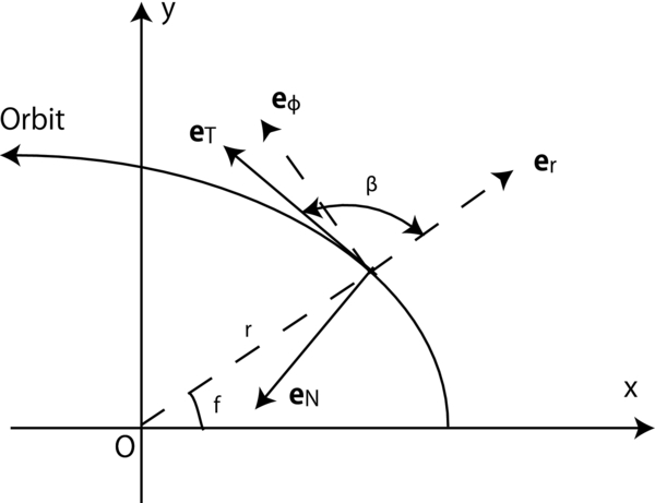
Figure 3. Definition of unit vectors  and
and  and their relations with the unit vectors in the cylindrical coordinates
  and
and  . The angle between
  and
and  is β.
is β.
Download figure:
Standard image High-resolution imageIn Figure 4, we show the evolution of the relative velocity vector  over one orbital period with e = 0.5. The planet feels headwind at the perihelion, and tailwind at the aphelion. Figure 5 shows the amplitude of the relative velocity over one orbital period. It is noted that if the planet's eccentricity exceeds the disk aspect ratio, the relative velocity is always supersonic, regardless of the position in the orbit.
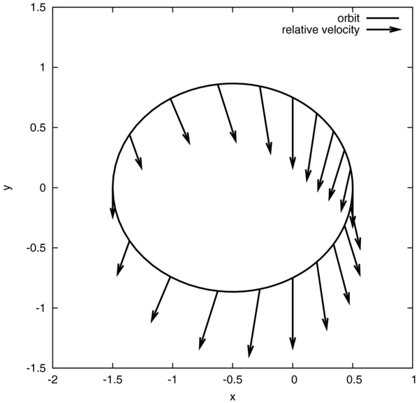
Figure 4. Evolution of the relative velocity vector along the planetary orbit with e = 0.5. The solid line shows the orbit of the planet, and the arrows show the direction of the relative velocity vector between the gas and the planet. We have assumed that the central star is at the origin, and the planet and the disk are both rotating in a counterclockwise direction.
Download figure:
Standard image High-resolution image
Figure 5. Amplitude of relative velocity between the gas and the planet over one period. The horizontal axis shows the true anomaly f, and the vertical axis shows the Mach number of the relative speed. The perihelion is at f = 0, and the aphelion is at f = π. The planet with eccentricity e = 0.01, 0.05, 0.1, 0.5, 0.9 is shown. We use the fiducial model (see the main text) for the gas disk.
Download figure:
Standard image High-resolution image3.3. Orbital Evolution of the Planet: Calculation Methods
We make use of Gauss's equations to calculate the orbital evolution of the planet. For the evolution of the semimajor axis and eccentricity, Gauss's equations read

and

where v is the speed of the planet and r is the distance between the planet and the central star. We denote the perturbing force per unit mass by (T, N), where T is the component of the force (per unit mass) in the tangential direction of the orbit (positive direction is the direction of the velocity), and N is the component in the plane of the orbit and perpendicular to T (positive direction is directed inside the orbital ellipse). The evolution equation for the true anomaly is given by

where η = (1 − e2)1/2, R is the component of the force in the radial direction, and S is the component perpendicular to R. Components (T, W) and (R, S) are related by

and

For the expressions of the perturbing force (T, W), we use the dynamical friction formula. In this paper, we especially focus on the planet with high eccentricity, and therefore assume that the relative speed between the gas and the planet is always supersonic. Therefore, we use the limiting form of a highly supersonic case, Equation (41). The amplitude of the force is

where Δv is the relative speed between the gas and the planet. The direction of the force is opposite to the relative velocity vector.
In order to find the long-term evolution of orbital parameters, we average Equations (59)–(61) over one orbital period assuming the planet is in a fixed orbit. Since the variation of a and e is very small over one orbital period, the assumption of a fixed orbit is justified. The averaging is done in such a way that

where Torb is the time taken over one period. The averaging is done in the same way for eccentricity.
3.4. Orbital Evolution of the Planet: Fiducial Model
In this section, we compare our results with previous numerical calculations for the fiducial model.
We first show the torque and power exerted on the planet by the disk over one orbit. The power  exerted on the planet is given by

and the torque  is
is

where  ,
,  , and
, and  are the position vector of the planet from the disk, the velocity of the planet, and the force exerted on the planet, respectively. In Figure 6, we show
  and
and  normalized by the planet's energy (the sign inverted),

and the angular momentum,

respectively.

Figure 6. Power  (left panel) and torque
  (right panel) exerted on the planet with eccentricity e = 0.3 (solid line) and e = 0.5 (dashed line). The fiducial model is used. For the power we plot
  , and for the torque we plot
  , where Ep and Lp are the planet's energy and angular momentum, respectively, and n is the mean motion of the planet. The horizontal axis shows the true anomaly f, and f = 0 corresponds to the perihelion.
Download figure:
Standard image High-resolution imageIn the vicinity of the perihelion, the torque and the power are negative because of the headwind toward the planet, and they are positive in the vicinity of the aphelion owing to the tailwind. Similar behavior is observed in the numerical simulations of Cresswell et al. (2007). The behavior of the torque exerted on the planet looks very similar except for the small difference between the location of the perihelion or aphelion and the location of the maximum or minimum of the torque (see Figure 8 of Cresswell et al. 2007). In our model, this small difference in phase does not appear since we assume that the force is proportional to the relative velocity at the location of the planet.
The comparison of our results with Figure 10 of Cresswell et al. (2007) shows that the behavior of the power is very different. This difference cannot be attributed to the sets of parameters they have used different from our fiducial model. This may be because our model for the force exerted on the planet is very simplified. This difference in power leads to the different behavior in da/dt and de/dt over one orbital period, which is shown in Figure 7. We note here that the evolution of eccentricity is qualitatively different from Figure 9 of Cresswell et al. (2007). Fortunately, however, it is possible to obtain quantitatively the same results with previous numerical calculations when we take the average over one orbital period, as shown below.

Figure 7. Evolution of the semimajor axis da/dt (left panel) and eccentricity de/dt (right panel) of the planet with eccentricity e = 0.3 (solid line) and e = 0.5 (dashed line). The fiducial model is used. For the evolution of the semimajor axis, we plot (da/dt)(1/na)/(Mp/M*), and for the evolution of eccentricity, we plot (de/dt)(1/n)/(Mp/M*). The horizontal axis shows the true anomaly f, and f = 0 corresponds to the perihelion.
Download figure:
Standard image High-resolution imageFigure 8 shows the results of migration rate tm and eccentricity damping rate te, which are obtained by averaging over one orbital period. Also plotted in this figure is the formula obtained by Papaloizou & Larwood (2000) given in Equations (48) and (49). For the migration rate, we also show tm given by Papaloizou & Larwood (2000) times 3/2 for e < 0.5, which describes the results of numerical simulations better as noted by Cresswell & Nelson (2006). For the damping of eccentricity, the formula by Papaloizou & Larwood (2000) fits the results of numerical simulations well. We see that our results for te agree very well with the formula by Papaloizou & Larwood (2000) for e ≲ 0.7. For the migration rate, our formulation consistently results in a timescale slower by a factor of two compared to the numerical simulations. Our results deviate from those of Papaloizou & Larwood (2000) for large values of eccentricity. We expect that our treatment is actually better for highly eccentric cases (discussed in later sections), and that this difference is attributed to the breakdown of the expansion of e used by Papaloizou & Larwood (2000).
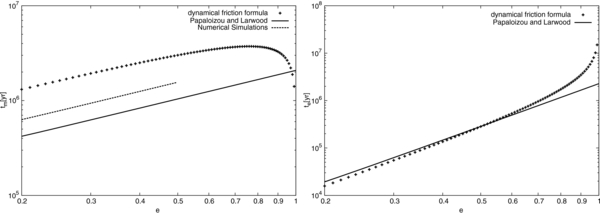
Figure 8. Migration timescale tm (left) and eccentricity damping timescale te (right) for the fiducial model. For both of the panels, we compare our results (crosses) and the formula by Papaloizou & Larwood (2000: solid line). For tm, we also show the formula of Papaloizou & Larwood (2000) multiplied by 3/2 with the dashed line for e < 0.5, which Cresswell & Nelson (2006) claim to better fit the results of numerical simulations.
Download figure:
Standard image High-resolution image3.5. Orbital Evolution of the Planet: Varying Disk Model
We have seen that our formulation results in a consistent timescale of the evolution of orbital parameters for the fiducial model. We now look at how the timescales behave as we vary the disk model.
In our framework, the force exerted on the planet can be written in the form

and

where K and α are constants. For the model of the force we use in this paper, which is Equation (64), if we use the softening parameter proportional to the disk scale height, = 0H(r), the constant K is given by

and α is given by

where H0 is the disk scale height at r = r0. Therefore, models with the same K and α yield the same results. In this section, we show the results of how ta and te depend on the disk profile p, or in more general terms, α. We fix the value of surface density to be Σ0/(M*/r20) = 10−4, the planet mass to be Mp/M* = 10−6, the disk aspect ratio to be H0/r0 = 0.05, and the softening parameter to be 0 = 0.5. The dependence of these parameters on the timescales ta and te is t∝M−1pΣ0−10H0, as expected from the form of K, as long as the force exerted by the disk is sufficiently small compared to that from the central star. We use the disk model with q = 1, which gives α = p + 1, but we note again that the value of α is the key parameter that determines the values of ta and te.
Figure 9 shows ta and te for α = 1, 2, 3, 4 (p = 0, 1, 2, 3, respectively, for q = 1). In Figure 9, we fix a/r0 = 1 and see how the timescale behaves as we vary the eccentricity. We see that the behaviors of ta and te strongly depend on the imposed disk model. The timescale of the evolution of the semimajor axis increases steadily as we increase eccentricity if α ⩽ 2. If, on the other hand, α ⩾ 2, the values of ta first increase as we increase e, but decrease at large e. The timescale of the evolution of eccentricity always increases as we increase eccentricity if α ⩽ 3, but there is a maximum of te at a certain value of e if α > 3.
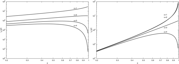
Figure 9. Timescale of the evolution of the semimajor axis ta (left) and timescale of the evolution of eccentricity te (right) for the models with α = 1, 2, 3, 4 (p = 0, 1, 2, 3, respectively, for q = 1). The lines for α = 1 and α = 2 are almost identical for te. We take a/r0 = 1, and the unit of the time is year with r0 = 1 AU and M* = M☉. The direction of the semimajor axis evolution is inward, and the eccentricity always damps.
Download figure:
Standard image High-resolution imageAs we decrease the values of α, another interesting behavior occurs for ta. In Figure 10, we show the behavior of ta and te for α = −1, 0, 1 (p = −2, −1, 0). We see that the timescale of the eccentricity evolution does not vary much within this parameter range, while ta is negative for almost all the values of e for α = 0 and −1. The negative sign of ta indicates that the direction of the semimajor axis evolution is outward.

Figure 10. Timescale of the evolution of the semimajor axis ta (left) and timescale of the evolution of eccentricity te (right) for the models with α = −1, 0, 1 (p = −2, −1, 0, respectively, for q = 1). We take a/r0 = 1 and the unit of the time is year with r0 = 1 AU and M* = M☉. For clarity, the left panel shows 1/ta, since the sign of the direction of the semimajor axis evolution changes. The negative sign indicates that the direction of the semimajor axis evolution is outward. Eccentricity always decreases for the parameters presented here.
Download figure:
Standard image High-resolution imageThe reason why we obtain the outward semimajor axis evolution can be qualitatively explained as follows. If the index p is negative, the surface density increases as a function of radius. As we have seen before, the planet feels the tailwind at the aphelion and therefore is exerted positive torque by the gas, while it feels headwind at the perihelion and is exerted negative torque. Since the surface density is larger at the aphelion than at the perihelion when p is negative, the planet feels overall positive torque, and therefore the semimajor axis increases.
The disk with negative p seems rather unrealistic. However, the surface density may increase locally as a function of radius. The inner edge of the disk is one example in which such local increase of the surface density is expected. If a planet with a finite eccentricity is placed in such a place, we expect that the semimajor axis can increase as a result of the disk–planet interaction. Recently, Ogihara et al. (2010) have suggested that the planets trapped in mean motion resonances can be stopped at the disk inner edge. This is because at the gap edge, the planet feels the disk only at the place close to the aphelion; therefore, it is exerted the positive torque by the disk. This positive torque is balanced by the negative torque exerted by the other planet in a mean motion resonance.
3.6. Analytic Considerations for e ∼ 1
We have seen how the timescales of the semimajor axis evolution and the eccentricity damping vary as we change the disk parameter. Specifically, we have seen a strong dependence of ta and te on the disk parameter α = p + (3 − q)/2 if the planet eccentricity is high. In this section, we analytically investigate the behaviors of ta and te in the limit of e → 1.
In this section, we approximate df/dt (see Equation (61)) by

since the contribution from the perturbing force is small compared to the force from the central star. We then obtain

and
From Figure 7, we see that the force exerted when the planet is near the aphelion and the perihelion is important in determining the orbital evolution of the planet. We therefore look at the places close to the perihelion or aphelion. Around these points, cos f and sin f are approximated by


where we write f = δf near the perihelion and f = π + δf near the aphelion, and the upper sign is for the perihelion and the lower sign is for the aphelion. We expand Equations (75) and (76) up to the second order of δf. After the expansion with respect to δf, we take the limit of e → 1. We define

and take the lowest order of ε.
The calculations are tedious but straightforward. In the close vicinity of the perihelion, we obtain

and

We then integrate over the orbit. We denote the integral by

If we integrate over f, the terms in Equations (80) and (81) that contain δf result in a numerical factor of the order of unity. Therefore, close to the perihelion, da/df and de/df averaged over one orbital period are

and

We now turn our attention to the aphelion. In the close vicinity of the aphelion, we obtain

and

We now integrate over f near the aphelion. The integration for da/df is rather complicated. We have

and changing the integration variable to X = δf/ε1/2,

If ε is sufficiently small, the numerator is dominated by the second term, and therefore the resulting  is negative and
  . If ε is not very small, the numerator is dominated by the first term. Therefore the resulting integral is positive and
  . Therefore, the contribution of the aphelion to
  is
is

The integration for de/df is more straightforward. We have

and changing the variable to X = δf/ε,

The terms proportional to ε1/2 and ε are safely neglected, and therefore we have  . Therefore, for the contribution from the aphelion to
  , we have

It still remains to be determined whether contributions from the perihelion or from the aphelion dominate. The relative importance of the contributions from the aphelion and the perihelion depends on the disk model, and we numerically see which contribution is more important as we change α. In Figure 11, we plot the values of  and
and  for various disk models. We see that the contribution from the perihelion dominates when α ≳ 2 (corresponding to p ≳ 1 if q = 1), and the expected behaviors of
  and
and  are observed. If α ≲ 2, the contribution from the aphelion comes into play, and we see
  is roughly proportional to ε1/2. We note that for the models with α = −1 and α = 0, the direction of semimajor axis evolution is outward for the moderate values of eccentricity (ε > 0.09 for the α = 0 model and ε > 0.05 for α = −1), as we have already seen in the previous section. The inversion of the sign of
  is also expected from the above analytic discussions of the aphelion. We have also checked that the values of
  are always positive if we have a large negative value of p, when the interaction is completely dominated by the contribution from the aphelion.

Figure 11. Orbit-averaged values of −da/df (left) and −de/df (right) for various eccentricity and disk parameters with a/r0 = 1. The power p (the parameter α = p + 1 in the case of q = 1) of the surface density is varied and denoted in the figures. The horizontal axis shows the values of 1 − e. For da/df, the absolute values are plotted if −da/df is negative. For only the cases in which α = −1 and α = 0 with large values of 1 − e (1 − e > 0.09 for α = 0 and 1 − e > 0.05 for α = −1), we obtain negative values of  . The values of −de/df are always positive.
Download figure:
Standard image High-resolution image
We summarize the dependence of the semimajor axis evolution timescale and eccentricity damping timescale on the disk parameters in the case of a highly eccentric planet. Since  and
and  are related by

 . In the same way, it is possible to show that
  , where we have used e ∼ 1. In the case of α ≳ 2, the contribution from the perihelion dominates and therefore,


The evolution of the semimajor axis is always inward and the eccentricity always damps. If α ≲ 2, we take into account the contribution from the aphelion,

and

It is noted that the outward evolution of the semimajor axis occurs only when α ≲ 0, and eccentricity always damps. The range of ε where the planet experiences the outward semimajor axis evolution increases as the value of α is decreased. In the particular disk model with q = 1, α and p are related by α = p + 1.
We have shown that there is a critical value for the power of the surface density, which determines the behavior of semimajor and eccentricity evolutions for a highly eccentric planet (e ∼ 1). Let us consider the model with q = 1. If p > 2, both eccentricity and semimajor axis evolution timescales become small as we increase the planet's eccentricity. If 1 < p < 2, the semimajor axis evolution timescale becomes shorter for higher eccentricity, while the eccentricity evolution timescale becomes longer. For p < 1, both evolution timescales become longer as we increase the eccentricity of the planet. Further complications arise for the semimajor axis evolution for p ≲ 0, where the contribution from the aphelion comes into play to invert the direction of the evolution.
However, we note that these critical values of p should not be overstated. In the model described above, the critical parameter that determines the behavior of the orbital evolution timescales is α = p + (3 − q)/2. The appearance of this single parameter α is partly due to the prescription of the cutoff of the gravitational force. Note that the dynamical friction force we have used depends on the cutoff scale , and we have used the model in which depends linearly on the disk scale height. The appearance of q in the parameter α depends on this simplified prescription of the cutoff. We also note that the dependence of the timescales on the softening length is different from Papaloizou & Larwood (2000), which is due to the difference in the formulation.
Therefore, we consider that the critical values of p described above only have qualitative meanings. Yet, we expect that the model describes the qualitative behavior of the semimajor axis and the eccentricity evolution of highly eccentric planets. The prediction is readily compared with two-dimensional numerical calculations, although a very large simulation box may be necessary. In order to eliminate the dependence on the softening parameter , it is necessary to perform three-dimensional analyses.
3.7. Validity of the Model
In this section, we briefly discuss the applicability of our model. The most important assumption we have used in the model is the use of the supersonic dynamical friction formula (41), which is derived from linear perturbation analyses. The use of this formula assumes that (1) the relative velocity is supersonic, (2) the flow in the vicinity of the planet is homogeneous, and (3) the steady state is reached instantaneously. We shall now discuss each assumption separately. We will also discuss how nonlinear effects on the dynamical friction force may change our results.
The first assumption is justified if we consider a planet that has high enough eccentricity, as indicated in Figure 5. Typically, when e ≫ H/r, we can safely assume that the flow is supersonic.
For the second assumption, let us consider which scale of the perturbation contributes to the force. In the discussion of Section 2, we have seen that the perturbation of all the scales larger than the cutoff length equally contribute to the dynamical friction force. Let us consider a planet embedded in a disk with Keplerian rotation, located at the perihelion or aphelion. Then, there is a location in the disk where the relative velocity between the gas and the planet becomes zero. We call this radius an "instantaneous corotation radius," rC, given by, for the perihelion,

A similar equation can be derived for the aphelion.
The assumption of the homogeneous flow breaks down if the length scale comparable to the distance between the planet's location and the instantaneous corotation radius is important in determining the force acting on the planet. If the planet's eccentricity is large, the distance between the instantaneous corotation radius rC and the planet's location is of the order of the scale of the disk itself (|rC − a| ∼ a), which is much larger than the cutoff scale, which is comparable with the disk scale height. Therefore, in this case, we expect that the assumption of the homogeneous flow is justified. If the planet's eccentricity is small, the instantaneous corotation radius comes very close to the planet's orbital radius (rC ∼ a), and the assumption of a homogeneous medium becomes worse. Typically, we expect that this assumption breaks down if the planet's eccentricity is smaller than the disk aspect ratio, and in such a small eccentricity case, it is necessary to fully take into account the effects of shear around the planet's location.
Regarding the third assumption, the time taken to reach the steady state may be estimated as follows: The length scale that is important in determining the force is of the order of the disk scale height, and the minimum speed of the propagation of the information of the perturbing potential may be the sound speed. This indicates that the time taken to develop the steady state is of the order of the Kepler timescale. However, since the relative velocity is supersonic, the time taken to develop the steady state is less than that, since the background flow will carry the information of the perturber. In any case, this assumption is only marginally satisfied.
As previously discussed, it is known from numerical simulations that the time when the maxima/minima of the torque occurs lags the time of the maxima/minima of the distance between the planet and the central star (e.g., Cresswell et al. 2007). Our model does not give a precise prescription for these effects, and the instantaneous torque or power profiles are different from what we expect from the numerical simulations. However, if we take the average over one orbital period, our model is in good agreement with the previous calculations in the parameter range where both our model and the previous calculations are expected to give reasonable results.
In short, we expect that our formulation is applicable to planets whose eccentricity is larger than the disk aspect ratio, in particular when one takes the average over one orbital period.
Finally, we must make a comment on the use of the dynamical friction formula derived by the linear perturbation analysis. Kim & Kim (2009) investigated the dynamical friction using the nonlinear numerical simulations. They considered the case in which the particle is embedded in a homogeneous, three-dimensional gas flow, and calculated the axisymmetric pattern of the gas flow induced by the particle's gravity. They found that there is a deviation from the linear theory depending on the Mach number M0 of the flow and the nonlinear parameter

where rS is the (effective) radius of the body. The force exerted on the particle is deviated from the linear results by a factor of (η/2)−0.45, where  . In the case of a planet embedded in a protoplanetary disk,
  is of the order of 10–100; therefore, nonlinearity can be important. The correction factor, however, is the quantity of the order of unity, (since the Mach number is of the order of 5–10); therefore, our results may give a reasonable estimate of the timescale of the evolution of the orbital parameter. One possible effect of such nonlinearity on our results is that the dependence of the timescales ta and te on the orbital parameters of the planet can be different, since the force depends on the velocity of the perturbing potential in a different way.
4. DISCUSSION: POSSIBLE APPLICATIONS TO OTHER STUDIES
In this section, we discuss some possible applications of our results to other studies and the implications for the planet formation theory. We first show the fitting formula for ta and te derived from this study, which can be especially useful for population synthesis models such as those in Ida & Lin (2008). We then discuss some implications from this study for recent planet formation scenarios.
4.1. Fitting Formula for the Timescale of Semimajor Axis and Eccentricity Evolution
In this section, we derive the fitting formula for ta and te. As seen before, within our framework, ta, te∝M−1pΣ−100H0, and the only disk parameter that controls the timescale is α = p + (3 − q)/2. Therefore, we fit the values of ta and te as a function of the semimajor axis and the eccentricity for a given value of α with 1 ⩽ α ⩽ 4. For the data for fitting, we use the values obtained for 0.3 ⩽ a/r0 ⩽ 10 and 0.1 ⩽ e ⩽ 0.99.
Motivated by the results of the analytic considerations for e ∼ 1, we use the fitting formula of the form

Here, Ca, ζa, λa, and ηa are the function of a of the form


The same form of the fitting function is used for te,

with


We note that in the set of the fitting parameters, Ca0 and Ce0 have the dimension of time, while others are dimensionless.
In Tables 1 and 2, we show the results of fitting for ta and te, respectively. For Ca0 and Ce0, we give the values in the units of year with M* = M☉ and r0 = 1 AU. In the last column of the tables, we show the maximum values of the error of the fitting function, which is calculated as |tcalc − tfit|/tcalc, where tcalc is the value of ta or te calculated in the model presented in this paper and tfit is the value of the fitting function. Our fitting formula successfully reproduces the values of ta and te within a 10%–20% error. We also note that aα − 3/2 dependence that appears in Equations (94)–(97) can be seen clearly in the fitting parameters Cap and Cep.
Table 1. Fitting Results for ta
| α | Ca0 (yr) | Cap | ζa0 | ζap | λa0 | λap | ηa0 | ηap | Max. Error |
|---|---|---|---|---|---|---|---|---|---|
| 1.0 | 3.789E+06 | −5.241E−01 | 9.759E−01 | −1.471E−05 | 1.320E−03 | −1.211E−01 | −1.986E−01 | 3.019E−09 | 1.886E−01 |
| 1.5 | 3.762E+06 | 4.353E−07 | 8.977E−01 | 3.777E−08 | 1.658E−01 | 2.010E−06 | −2.173E−01 | 1.068E−09 | 3.895E−02 |
| 2.0 | 3.988E+06 | 5.000E−01 | 1.008E+00 | −1.188E−09 | 1.129E+00 | 7.216E−08 | 5.318E−02 | 3.436E−09 | 4.497E−03 |
| 2.5 | 2.861E+06 | 1.000E+00 | 9.952E−01 | 0.000E+00 | 2.112E+00 | 0.000E+00 | 4.984E−01 | 0.000E+00 | 2.038E−03 |
| 3.0 | 2.265E+06 | 1.500E+00 | 9.944E−01 | 0.000E+00 | 2.063E+00 | 0.000E+00 | 9.957E−01 | 0.000E+00 | 2.787E−03 |
| 3.5 | 1.948E+06 | 2.000E+00 | 1.010E+00 | 1.604E−10 | 1.920E+00 | −3.424E−10 | 1.503E+00 | −4.489E−11 | 3.085E−03 |
| 4.0 | 1.793E+06 | 2.500E+00 | 1.041E+00 | 6.360E−10 | 1.774E+00 | −1.094E−09 | 2.012E+00 | −1.386E−10 | 1.058E−02 |
Download table as: ASCIITypeset image
Table 2. Fitting Results for te
| α | Ce0 (yr) | Cep | ζe0 | ζep | λe0 | λep | ηe0 | ηep | Max. Error |
|---|---|---|---|---|---|---|---|---|---|
| 1.0 | 3.426E+04 | −5.090E−01 | 2.651E+00 | −1.908E−06 | 1.158E−03 | −1.331E−02 | −6.765E−01 | 8.473E−10 | 8.247E−02 |
| 1.5 | 3.768E+04 | −9.810E−02 | 2.615E+00 | −3.975E−05 | 2.431E−03 | −1.324E−01 | −7.394E−01 | −2.246E−08 | 1.126E−01 |
| 2.0 | 3.307E+06 | 5.000E−01 | 2.914E+00 | 0.000E+00 | 1.258E+00 | −9.885E−11 | −7.597E−01 | 0.000E+00 | 5.556E−02 |
| 2.5 | 3.956E+06 | 1.000E+00 | 2.984E+00 | 0.000E+00 | 1.733E+00 | −4.559E−11 | −5.236E−01 | 0.000E+00 | 9.257E−03 |
| 3.0 | 2.372E+06 | 1.500E+00 | 2.991E+00 | 0.000E+00 | −7.393E−09 | −5.798E−09 | −2.964E−02 | 0.000E+00 | 1.802E−02 |
| 3.5 | 4.528E+06 | 2.000E+00 | 3.038E+00 | 0.000E+00 | 1.376E+00 | −5.197E−10 | 5.102E−01 | 0.000E+00 | 9.239E−03 |
| 4.0 | 7.059E+06 | 2.500E+00 | 3.183E+00 | 0.000E+00 | 8.549E−01 | −5.166E−10 | 1.027E+00 | 0.000E+00 | 2.573E−02 |
Download table as: ASCIITypeset image
Here, we note that caution must be paid in using the fitting formulae. In obtaining the fitting parameters, we have used the values with 0.3 ⩽ a/r0 ⩽ 10 and 0.1 ⩽ e ⩽ 0.99. Our formulation is not applicable to the case of a low-eccentricity planet (typically e ≲ H/r). It is necessary to combine the results of this paper and such formulae given by Tanaka & Ward (2004), which are applicable to the case of low eccentricity.
It is also noted that the fitting formulae are given in the case of 1 ⩽ α ⩽ 4. Our form of fitting functions (100) and (105) fails to describe the change of the sign of ta that happens in the case of p ≲ −1 (see Figure 11). Although we believe that this range of α covers most of the typical protoplanetary disk parameters, it is necessary to construct the fitting formula if one wants to apply for protoplanetary disk parameters out of the range of this fitting. Even in this case, however, we expect that the model described in this paper, which uses the dynamical friction force to calculate the evolution of orbital parameters, is still applicable.
4.2. Implications for Planet Formation Theory
We have developed a model for the disk–planet interaction that can be used specifically for highly eccentric planets. We have found that in the case of a highly eccentric planet, the disk–planet interaction is essentially described by dynamical friction. We have derived how the evolution timescales of the planet's semimajor axis and eccentricity depend on disk parameters within our models. In this section, we discuss the possible implications for the planet formation theory.
Recently, Machida et al. (2011) suggested that a disk surrounding a newly born protostar is gravitationally unstable, and that it therefore may be possible to form a planet through gravitational instability (see also Inutsuka et al. 2010). Planets born in such a way are expected to have high eccentricity. Also, it is possible to form a planet at a large distance from the central star.
We briefly discuss the evolution timescale of such planets. From the fitting formula of the evolution timescales, it is possible to show that the orbital evolution timescales of the newly born Jupiter-mass planets through the gravitational instability can be very rapid, since the disk is very massive compared to the central star. However, after the accretion phase onto the central star, the stellar mass becomes much larger than the disk mass. If there is a low-mass planet (e.g., a sub-Jupiter mass) that has survived in the early phase and a reasonable amount of eccentricity is maintained, the orbital evolution timescale can be of an order of magnitude comparable with the observed disk lifetime (Haisch et al. 2001). Such planets may be found by the direct imaging observations (e.g., Marois et al. 2008), although small mass planets may be very cold and the observations may be difficult. Nevertheless, a highly eccentric planet at a large orbital separation can be a good observational signature to test the theory of the planet formation and disk–planet interaction.
Another possible mechanism for producing a planet in a highly eccentric orbit is planet–planet scattering (e.g., Chambers et al. 1996; Marzari & Weidenschilling 2002). The scattering between planets can naturally result in highly eccentric planets. From the calculations given in this paper, the evolution timescale of the orbital parameters can be very long even if the planet's orbital plane coincides with the gas disk plane. If the planet's orbital plane is not aligned with the plane of the disk, we expect that the evolution timescale becomes much larger, since the planet interacts with the disk only at a very small part of the orbit. The calculations given in this paper set the lower limit of the timescales of the orbital evolution for such planets. It is therefore possible that the scattered planets remain in a highly eccentric orbit, even if the gas disk remains and the tidal interaction with the central star is not effective.
Another interesting application of our model is the recently suggested "eccentricity trap" mechanism in Ogihara et al. (2010). They have suggested that if there is an inner cavity in a protoplanetary disk, it may be possible to maintain a planet at the inner edge of the disk. This is due to the positive torque acting on the planet at the aphelion, which stops the planet from migrating inward. Although our formulation, which assumes a smooth disk profile, is not directly applicable to the disk with a sharp inner edge, we have already seen that the evolution of the semimajor axis can be outward if there is a steep surface density gradient. It is an interesting extension to apply the method of dynamical friction to a disk with a cavity.
5. SUMMARY
In this paper, we have presented a model of disk–planet interaction that makes use of the dynamical friction force. This method can be especially useful for a highly eccentric planet.
We first derived the dynamical friction formula in a slab medium using different methods from Ostriker (1999) and calculated the dynamical friction force as a function of viscosity and Mach number. The integral that leads to the dynamical friction force is given by Equation (24), and some asymptotic expressions are given by Equations (28), (30), (40), and (41).
We then applied the dynamical friction formula to find the evolution of orbital parameters of an eccentric planet embedded in a disk. The results agree well with the previous calculations given by Papaloizou & Larwood (2000) for moderate eccentricity (e ≳ H/r), and we expect that it is possible to use our model for much higher eccentricity. In this sense, this paper provides a complement to the previous study. We have seen that the evolution of the orbital parameters depends on the disk structure and have calculated some critical values for p, the power of the surface density profile, at which the behaviors of the timescales of orbital evolutions are qualitatively altered.
The model presented in this paper is restricted to a planet with high eccentricity, typically e ≳ H/r. It is also necessary that the disk profile is smooth in the vicinity of the planet, in order to justify the use of the dynamical friction formula, which is obtained under the assumptions of a homogeneous slab.
T.M. thanks Clément Baruteau for useful discussions. This work was supported in part by the Grants-in-Aid for Scientific Research 22·2942 (T.M.) and 20540232 (T.T.) of the Ministry of Education, Culture, Sports, Science, and Technology (MEXT) of Japan.
APPENDIX A: TIME-DEPENDENT ANALYSIS OF DYNAMICAL FRICTION FORCE
In this appendix, we perform a time-dependent linear analysis for the gravitational interaction between a slab and an embedded particle. We do not perform the analysis in full details. The objective of this section is to show that it is sufficient to perform the steady-state analysis in order to obtain the dynamical friction force.
We start with Equation (8) and perform the Fourier transform in the spatial direction via Equations (16) and (17). We then obtain an ordinary differential equation in time as

We consider that at time t = 0, the particle is suddenly switched on,

We define p, q, S (they should not be confused with p and q in the main text) as


and

So Equation (A1) can be written in a concise way

where we have also removed the tilde sign for convenience. This equation should not be confused with that in the real space.
If we define the function g by

Equation (A6) becomes

where  .
.
The boundary condition is that there is no perturbation at t < 0. The solution that satisfies this condition is readily obtained as

where
are the homogeneous solutions. From Equation (A9), we can write the solution of α(t) as

We first note that the arguments in the exponential in Equation (A11) are given by

therefore, the real part is always positive in the presence of viscosity. Therefore, in the limit of t → ∞, the contribution from the last two terms in Equation (A11) vanishes if there is a viscosity, and the steady-state solution

is reached.
We now discuss the inviscid case, where the last two terms in Equation (A11) oscillate. We show that, even in this case, the contribution to the dynamical friction force coming from these time-dependent terms vanishes as t−1.
The expression of dynamical friction force (20) still holds in the time-dependent analysis. Therefore, we investigate the integral

where the factor e−k/k comes from the Fourier transform of the gravitational potential. In the case of an inviscid gas, the surface density perturbation is given by
We consider the terms in the integral (A14) involving the time dependence, which are the second and the third terms in the curly brackets of Equation (A15). Changing the variables as in Equations (22) and (23), we obtain the terms that are proportional to

where n = 1 for the second term and n = 2 for the third term. We further change the variable from k to ψ = ckt, and perform the integration over ψ. We now have

where we have taken the imaginary part that contributes to the dynamical friction force. The integral involved in Equation (A17) is finite for all values of t > 0, and asymptotes to a finite value as t → ∞. Therefore, the contribution to the force arising from the time-dependent terms decays as t−1, which justifies the steady-state assumption given in the main text.
APPENDIX B: THE EXACT EXPRESSION OF Iθ
The integral given by Equation (25) can be performed analytically. We make use of the software Mathematica to calculate the integral, and we show only the results in this section. The integral is given by

where the numerator is
and the denominator is

Footnotes
- 2
Here, "modified" means that they took the terms up to the second lowest order of H/r.
- 3
This is why Coulomb logarithm is involved in the dynamical friction formula.
- 4
The use of this value for rmin instead of the radius of the body is also motivated by the results of the collisionless system, where the 90° deflection angle appears as rmin.
- 5
It is noted that ta and tm are different by a factor of two even in the case of the circular orbit.