


ABSTRACT
Downward motions above post-coronal mass ejection flare arcades are an unanticipated discovery of the Yohkoh mission, and have subsequently been detected with TRACE, SOHO/LASCO, SOHO/SUMER, and Hinode/XRT. These supra-arcade downflows are interpreted as outflows from magnetic reconnection, consistent with a three-dimensional generalization of the standard reconnection model of solar flares. We present results from our observational analyses of downflows, which include a semiautomated scheme for detection and measurement of speeds, sizes, and—for the first time—estimates of the magnetic flux associated with each shrinking flux tube. Though model dependent, these findings provide an empirical estimate of the magnetic flux participating in individual episodes of patchy magnetic reconnection, and the energy associated with the shrinkage of magnetic flux tubes.
Export citation and abstract BibTeX RIS
1. INTRODUCTION
Supra-arcade downflows (SADs) are downward-moving features observed in the hot, low-density region above posteruption flare arcades. Initially detected with the Yohkoh Soft X-ray Telescope (SXT) as X-ray-dark, blob-shaped features, downflows have since been observed with TRACE (e.g., Innes et al. 2003a; Asai et al. 2004), SOHO/SUMER (Innes et al. 2003a), SOHO/LASCO (Sheeley & Wang 2002), and Hinode/XRT. The darkness of these features in X-ray and extreme-ultraviolet (EUV) images and spectra, together with the lack of absorption signatures in EUV, indicates that the downflows are best explained as pockets of very low plasma density, or plasma voids (see especially Innes et al. 2003a). Because these plasma voids are able to resist being filled in immediately by the surrounding ambient plasma, it seems reasonable to presume that magnetic flux within the voids provides supporting pressure. A configuration consistent with the observations is a magnetic flux tube, filled with flux but with very little plasma, shrinking into the posteruption arcade (McKenzie & Hudson 1999; McKenzie 2000). It is thus believed that the downflows represent the outflow of magnetic flux from a reconnection site, in keeping with the standard reconnection model of eruptive flares. The emptiness and motion of the plasma voids are consistent with flux tubes shrinking at rates exceeding the speed with which chromospheric evaporation can fill them with plasma (McKenzie & Hudson 1999; McKenzie 2002).
This interpretation does not conflict with the results of Verwichte et al. (2005). Verwichte et al. (2005) analyzed the oscillations of the supra-arcade rays in the 2002 April 21 flare observed by TRACE, and found that the oscillations can be described as sunward-traveling wave packets. That paper focused only on the oscillations in the rays, or "tails of the tadpoles," and did not speculate on the nature of the plasma voids, or "heads of the tadpoles." We have confirmed this interpretation of the paper through private communication with E. Verwichte (2008). The suggestion that Verwichte et al. (2005) offer an alternate interpretation of plasma voids arises from the imprecise nomenclature used in the paper, wherein "tadpole" sometimes refers to the head alone, and more often to the dark tail. We avoid the term "tadpole" because of this confusion, and also because the term conjures an image of a blob denser than its surroundings, contrary to the findings of Innes et al. (2003a).
The speeds of SADs reported previously (e.g., McKenzie & Hudson 1999; McKenzie 2000; Innes et al. 2003a; Asai et al. 2004) are on the order of a few ×101–102 km s−1, slower than canonically expected for reconnection outflows (i.e., slower than the 1000 km s−1 which is often assumed to be the Alfvén speed). Linton & Longcope (2006) suggest the possibility of drag forces working against the reconnection outflow to explain why the speeds are sub-Alfvénic. In their model, reconnection was allowed to occur for a finite period of time, in a localized region of slightly enhanced resistivity, and reconnected field was observed retracting away from the reconnection site: "this accelerated field forms a pair of three-dimensional, arched flux tubes whose cross sections have a distinct teardrop shape. We found that the velocities of these flux tubes are smaller than the reconnection Alfvén speed predicted by the theory, indicating that some drag force is slowing them down." Alternatively, plasma compressibility can reduce the speed of reconnection outflow (Priest & Forbes 2000). We show below that the observations do not appear to support an interpretation based on compressibility.
The sizes of the teardrop-shaped outflows of Linton & Longcope (2006) are determined by the duration of a given reconnection episode and by the size of the patch of enhanced resistivity. From the SAD observations, the sizes of the plasma voids can be directly measured and utilized as constraints in the model: ideally, the model would produce a distribution of outflowing flux tubes that mimics the distribution found in the observations. Additionally, their speed profiles (including acceleration/deceleration) may eventually be useful for understanding the nature of any drag forces.
Nearly all that is known about the supra-arcade region is of a qualitative nature. There is not in the literature any collection of the statistics of SADs. To be useful as constraints for the models, the observations must yield quantitative measurements with estimable uncertainties. Whereas most of the preceding literature about SADs has focused on their mere presence (e.g., McKenzie 2000), the fact that they are voids (Innes et al. 2003a), or their timing in relation to nonthermal energy release (Asai et al. 2004; Khan et al. 2007), in the present paper we report observational quantities from a sample of plasma voids in three flares, quantities which are potentially useful as model inputs or constraints. The distributions of observed void sizes and speeds are displayed. We combine the measured sizes with a model of the magnetic field in the supra-arcade region to yield estimates of the magnetic flux in individual flux tubes. We believe that these flux estimates—while admittedly subject to observational and model-dependent uncertainties—represent the first empirical estimates of the characteristic flux participating in individual reconnection events.
Linton & Longcope (2006) demonstrated that the energy released by the shrinkage of a flux tube accounts for a significant portion of the total energy released by an individual reconnection. Linton & Longcope (2006) indicate that for small reconnection regions the energy released by the loop shrinkage may in fact be considerably larger than the energy directly released by magnetic reconnection. Hudson (2000) conjectured that magnetic structures must contract (or "implode") as a consequence of energy loss, and provided an upper limit on the energy accessible via implosion. In the present paper, we utilize the paths of the downward motions of plasma voids and an estimate of the fluxes in each of the shrinking flux tubes to make an empirical estimate of this energy. Except for the approximation of change in volume, our expression for the shrinkage energy is mathematically equivalent to Hudson's. To our knowledge, this is the first time that flare observations have been used to derive empirical estimates of this particular mode of energy release.
2. AUTOMATED DETECTION ALGORITHM
For this project, semiautomated software for detection and measurement of SADs has been developed. The effort was motivated by a desire to measure reliably and objectively the characteristics of SADs in a large number of flares, with repeatable results. In Innes et al. (2003a) and Sheeley et al. (2004), SADs are displayed via sloped traces in stackplots constructed from slices of the images. The difficulties in automating this technique are significant. (1) The method requires pixels to be extracted from a virtual slit placed along the trajectory of the downflow, requiring prior knowledge of the existence and location of the downflow; so it is most appropriate for demonstrating the existence of a downflow, not for automatically detecting the downflow. (2) With the stackplot, automated measurements of the void's area are not provided; the area must be measured manually. (3) To detect downflows automatically with stackplots, the virtual slit must be placed across the paths of the suspected downflows, like a "finish line" parallel to the limb. This was done in Innes et al. (2003a). The insurmountable problem is that in low-cadence image sequences, fast-moving voids can skip over the virtual slit and thus fail to be detected crossing the "finish line." For these reasons, an improved and automated method is warranted.
Our detection routine finds plasma voids in a flare movie by searching for locally depressed signals ("troughs") in each image, and then attempting to match trajectories extending over some user-defined minimum number of images. To detect a trough in a given image, the program identifies any contiguous group of pixels that is darker than a user-specified threshold amount. When a trough exceeding a predefined minimum size is identified, the positions of all its constituent pixels are recorded, as is the position of the trough's centroid. This process is repeated for each image in the movie.
The next step is to determine whether the positions in consecutive images trace out trajectories of moving troughs. Two key assumptions are applied: (1) only trajectories that indicate motion toward the flare arcade are accepted. (2) Trajectories comprising fewer than N position points are rejected, with N typically set to 4. The former assumption reflects our present focus on SADs, but could be removed for searches of flows directed away from the Sun. The latter assumption is intended to ensure reliability of the results. We find that troughs observed in fewer than four successive images are more likely to be false detections. For reference, in the three flares considered in this paper, the number of position points for each visually verified trough ranges from 3 to 41. One result of this conservatism is that the fastest SADs may be overlooked, as they can pass through the field of view in just two or three frames. For the 2002 April 21 flare (see below), assuming N = 4 and a cadence of 1 image per 30 s, SADs traveling faster than ∼1600 km s−1 could have passed undetected. For the 2000 July 12 flare (also below), similar considerations imply a maximum detectable speed of ∼1800 km s−1. To compensate for gaps in the data sampling, as well as for momentary disappearances of voids due to, e.g., temporary increases in data noise, trajectories shorter than N points may be combined if the velocities (speed and direction of the trough) before and after the dropout are consistent.
All the trajectories meeting the above criteria are displayed for the user, with movie clips from the relevant image frames, to allow visual inspection and rejection of any false trajectories. Although the routine has been designed to find as many full-length tracks as possible, the noise in the region of interest makes this very difficult; therefore, manual tracking is enabled in order to allow the user to add to the automatically detected troughs. Upon acceptance by the user, the trajectories of detected troughs can be fitted with polynomials to obtain velocity and acceleration estimates. An additional product of the analysis is automated determination of the size of each plasma void, by counting the number of pixels associated with each trough and scaling by the telescope's angular resolution.
The routine has been refined through repeated application to synthetic flare data which mimic the appearance of downflows within a background of white noise. The noise level and parameters of the artificial voids (e.g., size, speed, and darkness) have been varied for the refinement of the analysis software. An example frame from one synthetic data sequence, designed to mimic the very low signal-to-noise ratio of the SXT downflow movies (significantly noisier than the TRACE data), is shown in Figure 1(a).
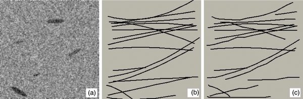
Figure 1. Testing the semiautomated software with an SXT-mimic synthetic data set. (a) Five artificial voids are seen in this frame. A total of 16 voids were created in this 50-frame movie. The actual trajectories of all 16 are shown in panel (b), and the trajectories as determined by the software are in panel (c).
Download figure:
Standard image High-resolution imageIn all tests of synthetic data, the routine was able to detect all the troughs; refinements to the software allowed elimination of false positives. Figure 1(b) and (c) demonstrate the trajectories of voids in the SXT-mimic synthetic data.
We note that in addition to the dark plasma voids, shrinking loops are often observed. These X-ray or EUV-emitting loops are observed in the same supra-arcade region with the plasma voids, often during the same time intervals, and moving at similar speeds. These loops appear to get brighter as they approach the top of the arcades. In such cases, it would appear that the "bright shrinkages" are observed because chromospheric evaporation fills the loops before/as they shrink, whereas voids appear dark because they are shrinking before evaporation has filled them. In the present work, we have focused on the plasma voids, rather than the "bright shrinkages", primarily because they are observationally easier to distinguish from the bright loops in flares.
3. ANALYSIS OF SOLAR FLARE DATA
The automatic detection routine has been applied to image sequences from three SAD flares, summarized in Table 1. All three were accompanied by coronal mass ejections (CMEs). The X1.5 flare of 2002 April 21 was observed by TRACE, RHESSI, SOHO, and numerous other observatories (e.g., Wang et al. 2002; Innes et al. 2003a). The 1999 January 20 M5.2 flare was observed by Yohkoh/SXT, and was the discovery event for downflows; this flare was described extensively in McKenzie & Hudson (1999) and in McKenzie (2000). The M5.7 flare of 2000 July 12 was observed by SXT. The TRACE images from April 21 have angular resolution of 0.5 arcseconds pixel−1, whereas the July 12 and January 20 images were made in SXT's half-resolution mode, corresponding to 4.91 arcseconds pixel−1. As a result, the smallest of the voids seen by TRACE would have been completely undetectable by SXT; this is borne out in the histograms of detected voids (see below). In all three flares, SADs were faintly visible in the raw images; the images were processed for contrast enhancement prior to application of the SAD-tracking routine.
Table 1. Summary Information of Flares Analyzed in the Present Work
| Date | GOES Start, Peak (UT) | GOES Classification | Source of Images | Time Span of Analysis (UT) |
|---|---|---|---|---|
| 2002 Apr 21 | 00:43, 01:51 | X1.5 | TRACE (195 Å) | 01:32–02:26 |
| 1999 Jan 20 | 19:06, 20:04 | M5.2 | SXT | 20:36–21:28 |
| 2000 Jul 12 | 18:41, 18:49 | M5.7 | SXT | 21:14–21:53 |
Download table as: ASCIITypeset image
In our preliminary reports of this research (e.g., in Conference Proceedings), speeds were based on the trajectories of the void centroids. In many observations of SADs, the plasma voids become elongated over time, producing the "tails" that stretch high into the corona. The physical reason for this apparent elongation is not yet clear; but whatever the cause, the result is that centroid velocities are more likely to underestimate the speed of the downflow. Although efforts are made to separate the tail from the "head" of each downflow, clear separation is not always possible. Therefore, we have calculated speeds from the tracked motion of the leading edges of the plasma voids, despite an increased dependence on detection threshold.
By fitting a parabolic polynomial to the trajectory of each void, the speeds and accelerations of each void can be measured. The accelerations are generally small, however, and subject to uncertainties in the position points. This is particularly true for cases where the automatically determined trajectories are noisy and span only a few position points. The plots in Figure 2 show the time profiles of the locations of two SADs from the April 21 flare, to demonstrate the range of scatter in the SAD trajectory determinations. For the purposes of the present paper, we have averaged the speed of each plasma void over its full measured trajectory, rather than presenting the velocities and accelerations derived from polynomial fits. The path-averaged speeds reported herein range from 28 to 263 km s−1 in the plane of the sky. We have not attempted to correct the velocities for projection effects. In a future paper (S. L. Savage et al. 2009, in preparation), we will explore the distribution of velocities more deeply, including accelerations and the spatial/temporal variations in SAD speeds from a larger number of flares. The purpose of reporting speeds in the present paper is to demonstrate the capability of the detection scheme.
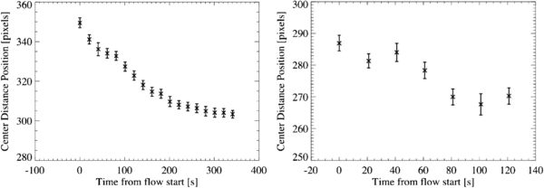
Figure 2. Example trajectories from two SADs detected in the April 21 flare, demonstrating the range of uncertainty in the trajectory determinations. The left-hand example is an SAD with very little scatter in the automatically determined trajectory; the right-hand example is one of the noisier trajectories. Velocities and accelerations can be derived from polynomial fits to the trajectories; however, for the present paper only path-averaged speeds are reported.
Download figure:
Standard image High-resolution imageSimilarly, the sizes of detected voids are averaged over the lifetime of each downflow. The findings from each flare are described below, with the trajectories of SADs shown in Figures 3, 4, and 5. To facilitate a side-by-side comparison of the speeds found in all three flares, the histograms from all three have been gathered together in Figure 6. The void sizes for all three flares are shown in Figure 7.
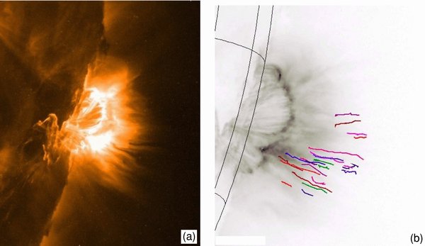
Figure 3. (a) Famous flare of 2002 April 21 revealed downflows in TRACE and SUMER for the first time, and represents one of the sharpest observations of downflows. (b) Downflows detected in the April 21 flare, tracked by the automated routine.
Download figure:
Standard image High-resolution image
Figure 4. Downflows detected in the January 20 flare, tracked by the automated routine. The solar limb is at right; the arcade itself is obscured by pixel saturation.
Download figure:
Standard image High-resolution image
Figure 5. Downflows detected in the July 12 flare, tracked by the automated routine. The solar limb is at left.
Download figure:
Standard image High-resolution image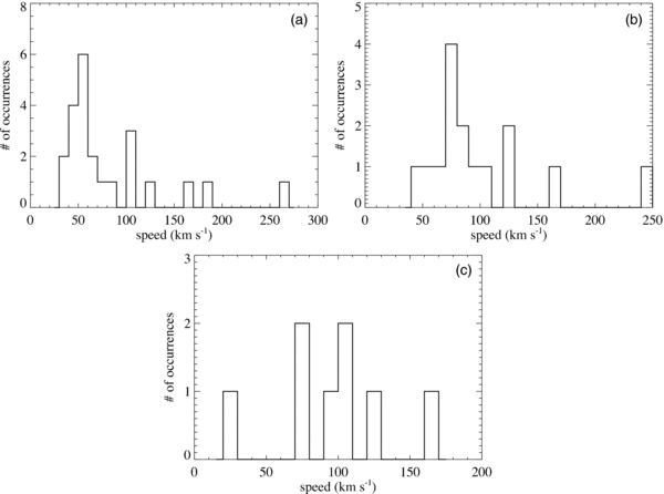
Figure 6. Distribution of speeds found in the detected downflows: (a) April 21 flare, (b) January 20 flare, and (c) July 12 flare.
Download figure:
Standard image High-resolution image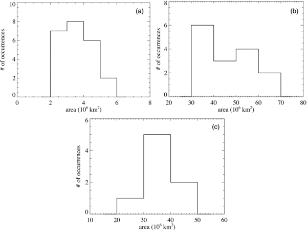
Figure 7. Distribution of areas found for the detected downflows: (a) April 21 flare, (b) January 20 flare, and (c) July 12 flare.
Download figure:
Standard image High-resolution image3.1. 2002 April 21,TRACE Data
In the TRACE data from 2002 April 21 (Figure 3(a)), the automated detection routine tracked 23 downflows which have been manually verified by visual inspection. The trajectories of the detected downflows are plotted in Figure 3(b). Although SADs descending into the southern part of the arcade were most obvious, and have been described elsewhere, the automated routine detected downflows above other parts of the arcade during the later part of the rising phase of the flare. Path-averaged speeds of the downward motions range from 38 to 263 km s−1 (Figure 6(a)). The median speed is 60 km s−1. Figure 7 shows the sizes of the detected X-ray voids. The median area is 3.5 × 10⁶ km2.
3.2. 1999 January 20, SXT Data
In the SXT data from 1999 January 20, 15 downflows were found above the arcade. The trajectories of the detected downflows are plotted in Figure 4. The downward speeds in this flare are very similar to those in the April 21 flare (Figure 6(b)); speeds range from 48 to 243 km s−1, the median speed being 81 km s−1. Due to the much coarser angular resolution of SXT compared with TRACE, and the very noisy signal in the flare images, none of the smaller SADs are detected: the median area among these SADs is 4.2 × 10⁷ km2 (Figure 7(b)).
3.3. 2000 July 12, SXT Data
In the SXT data from 2000 July 12, eight downflowing voids were tracked and manually verified; the trajectories are displayed in Figure 5. As in the January 20 flare, the detected plasma voids are larger than those in the April 21 flare; the median area is 3.8 × 10⁷ km2 (Figure 7(c)). This follows as a result of the vast difference in angular resolutions used for the respective images. The downflow speeds are shown in Figure 6(c). Path-averaged speeds range from 28 to 165 km s−1; the median speed is 104 km s−1.
Figure 7 demonstrates that in each flare a range of void sizes are detected. There is disparity between the three distributions in Figure 7—the TRACE images apparently reveal no voids larger than 10 × 106 km2, which are seen in the SXT flares. In an attempt to evaluate whether this disparity is related to the difference in angular resolution, we have rebinned the TRACE data to 2.5 arcsec pixel−1 to approximate the SXT full-resolution pixel size, and to 5 arcsec pixel−1 to approximate the SXT half-resolution pixel size. We observe in the unbinned TRACE images that it is possible to distinguish between the "tail" of an SAD and the slightly darker plasma void. When the images are rebinned to coarser angular resolutions this void/tail distinction is quickly destroyed. The result is that SADs in the rebinned data are given areas that include part of the "tail." The largest of the 2.5 arcsec binned SADs is ∼40 × 106 km2, similar to the median area found in the July 12 flare; the mode of the binned SADs is ∼10–20 × 106 km2. As the angular resolution of the images is further degraded, the voids become entirely undetectable. The brightness contrast between the voids (including the "tails") and the surrounding supra-arcade plasma is too low to allow the SADs to stand out in images where the angular width of a pixel is greater than the width of the SADs. In the 5 arcsec binned TRACE data, the voids are virtually undetectable, to the degree that no measurements of size or speed are possible. The same effect is seen in the quarter-resolution flare images from SXT (9.8 arcsec pixel−1), for nearly all flares observed by SXT.
From this exercise, we conclude that some of the areas measured in SXT images may include contributions from the SAD "tails" due to greater difficulty in separating "tail" from void. We see no reason why TRACE would not have detected voids as large as 30 × 106 km2 or larger, if they had been present in the April 21 flare. At the same time, we remark that each flare is different, and each may have a different range of SAD sizes.
4. DISCUSSION: RELATION TO RECONNECTION
It is generally accepted that magnetic reconnection is responsible for either the initiation or dynamical progression of CMEs and eruptive flares. Reconnection is the central component in the two-dimensional model due to Carmichael (1964), Sturrock (1968), Hirayama (1974), and Kopp & Pneuman (1976), sometimes called the CSHKP model, which continues to form the organizing element of much CME and flare research (see Shibata 1999, for a summary). It is a testament to this model that decades of observations and numerical simulations have not overturned it or even changed its basic form. In this section, we consider the measured characteristics of SADs in relation to quantities pertinent to reconnection.
4.1. Measured Speeds
The observed SAD speeds are slow in comparison to the 1000 km s−1 that is often assumed for the Alfvén speed. For an estimate of the Alfvén speed in the present flares, we utilize a PFSS magnetic field extrapolation (see below). At the locations of the detected SADs, the field strengths range between 10 G and 40 G (median 18 G). Assuming a plasma density of 109 cm−3 (e.g., Fletcher & Hudson 2008, and references therein), we infer Alfvén speeds of 690–2800 km s−1 (median 1200 km s−1). The downward motions thus appear to be sub-Alfvénic.
Linton & Longcope (2006) suggest that sub-Alfvénic outflows may result from drag forces. Although no attempt has been made here to estimate quantitatively the drag forces necessary to produce these speeds, the snowplowing suggested by Linton & Longcope (2006) could lead to enhanced density in front of the shrinking loop. Enhanced emission ahead of SADs has been noted by previous authors (e.g., Sheeley & Wang 2002; Innes et al. 2003b), though identification of this emission enhancement with snowplowing is highly speculative.
Alternatively, plasma compressibility can reduce the speed of reconnection outflow (Priest & Forbes 2000), by a factor of (ρi/ρo)1/2, where ρi (ρo) is the density upstream (downstream) of the reconnection. Comparison of the detected speeds to the median estimated Alfvén speed suggests reduction factors of 5–43 (i.e., detected speeds are 0.02–0.2vA). Such reductions would require density increases of 20–1800. The observed low density in plasma voids (Innes et al. 2003a), and lack of emission, are incompatible with density increases of such large magnitudes, suggesting that compressibility plays a negligible role.
4.2. Observed Sizes
In Linton & Longcope (2006), the size of the teardrop-shaped outflow is determined by the duration of a given reconnection episode and by the size of the patch of enhanced resistivity. The observed size distribution of downflow features may be useful for adjusting the parameters of such models.
We have already seen that SXT does not detect the smaller voids which are observable with TRACE, and we consider it likely that some plasma voids exist that are smaller than even TRACE can resolve. While the full range of possible diameters cannot be explored at present, we can explore the large-diameter end of the distribution. The histograms in Figure 7 demonstrate that for each flare a range of sizes exists, indicating that patches of reconnection may be found in a range of sizes. It is worth noting that the areas observed in these three flares are similar to the cross sections of reconnecting loops observed in TRACE by Longcope et al. (2005), wherein the median loop diameter was 3.7 Mm.
4.3. Estimation of Reconnecting Flux
For the April 21 and July 12 flares, the magnetic fields in the vicinity of the flares were retrieved from the PFSS extrapolations calculated by Dr. M. DeRosa (Schrijver & DeRosa 2003), provided within the SolarSoft (Freeland & Handy 1998) environment. The latitude, longitude, and height of the first detection of each plasma void were calculated by associating each void with a footpoint location, and by correcting the height for the effect of projection onto the plane of the sky. Because of the lack of obvious "legs" traceable from the voids down to the photosphere, the assignment of footpoint location introduces some uncertainty. For this first attempt at calculating loop fluxes, each plasma void was assumed to be situated radially above the "ribbons" of the arcade footpoints. The void's footpoint was identified as the point within the arcade's footpoints having position angle (measured counterclockwise from heliographic north) nearest to the position angle of the void. The heliographic latitude and longitude of the footpoint were then assigned to the void. The PFSS field strength at the position of the first detection of each plasma void was multiplied by the apparent size of the void to yield an estimate of the magnetic flux within the shrinking flux tube. This calculation was performed only for the two flares on the west limb: the magnetographic data upon which the PFSS extrapolations are based were more current for these flares than for the January 20 flare, which occurred on the east limb. Flux estimates are summarized in the histograms of Figure 8. Of the fluxes assigned to each SAD in the April 21 flare, the mean is 8.0 × 10¹⁷ Mx, the standard deviation of the mean is 1.0 × 10¹⁷ Mx, and the median is 7.1 × 10¹⁷ Mx. In the SADs of the July 12 flare, the mean flux is 5.9 × 10¹⁸ Mx, the standard deviation of the mean is 0.4 × 10¹⁸ Mx, and the median is 5.4 × 10¹⁸ Mx.
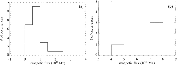
Figure 8. Distribution of magnetic fluxes found for the detected downflows: (a) April 21 flare, (b) July 12 flare.
Download figure:
Standard image High-resolution imagePotential sources of error in calculation of the magnetic fluxes include the height of each SAD above the photosphere, the cross-sectional area of its associated flux tube, and the strength of the magnetic field. The height of the reconnection event forming each shrinking flux tube is uncertain, due to noise in the images, threshold of the detection scheme, and projection effects (which we have tried to counter). Additionally, it is necessary to interpolate within the PFSS model to estimate the field strength at a given void's location. At the height of the SADs, the magnetic field strength varies smoothly, so that errors in the height of the void, or in the location of the footpoint, cause uncertainties on the order of 5%–20% of the field strength. An additional potential source of error is the fact that we assign a value corresponding to the height of initial detection, which is not necessarily the height of formation of the flux tube. As this height is a lower limit on the actual height of the reconnection site, it affects the flux determination because magnetic field strength falls with height. By underestimating height we may be overestimating flux. We use the area of a trough as a proxy for the cross-sectional area of the flux tube. The trough's area can be affected by noise in the images, as well as the sensitivity threshold of the detection. It is difficult to say whether this is systematically over- or underestimating the area, but we consider the area estimate to be accurate to within about 25%. We arrived at this estimation by repeatedly analyzing each of the flares, varying the threshold each time. The relative variation in the number of pixels identified with a given trough never exceeded 25%. We do not consider the effects of photon scattering in the telescopes, or the instrument point-spread function. Both scattering and a finite point-spread function reduce the contrast in the images, and could result in underestimating the area of a trough. Such effects are small in the SXT and TRACE images, and the associated uncertainty in the trough area is within the amount found by varying the detection thresholds.
The magnetic field estimate is derived from a PFSS extrapolation. The potential field extrapolation will tend to underestimate the strength of the magnetic field at heights above the active region, but a bigger source of uncertainty is the fact that these flares are at the limb. Since magnetograms are unreliable near the limb, the PFSS extrapolation employed uses only magnetograms within 55° of disk center, and then uses differential rotation and a surface transport code to model how the magnetic field evolves over the 3 days required to arrive at the limb. We consider that the PFSS field strength estimate is probably accurate to better than 30%, based on the following argument: in a recent analysis of nonlinear force-free field extrapolations for four flaring active regions, Regnier & Priest (2007) calculated the free energy in the nonlinear force-free fields, figured as the energy above that in the corresponding potential field, i.e., ΔE = Enlff − Epot. According to E. Priest (2007, private communication), these free energies ranged from ΔE/E = 0.023 to ΔE/E = 0.65, indicating differences in magnetic field strength of roughly ΔB/B = 0.01–0.3. Thus, the 30% uncertainty assigned to the PFSS field strength is reasonably conservative.
We note the similarity of the fluxes found here to that estimated by Longcope et al. (2005). In that work, reconnection appeared to proceed in "parcels of ∼4 × 10¹⁸ Mx at a time." It is difficult to say how much credence should be given to this similarity, because we know of no prediction in the literature of the amount of flux expected to participate in individual reconnection episodes. Work is in progress to perform this measurement for a larger number of flares, to determine whether the fluxes represented in Figure 8 are typical.
4.4. Inferred Reconnection Rate
Key to understanding the magnetic reconnection mechanism in flares is knowledge of the amount of magnetic flux that is processed over time—the reconnection rate. The reconnection rate has been measured indirectly by mapping the motions of chromospheric ribbons across magnetograms to determine the amount of flux that is input to reconnection (Saba et al. 2002; Fletcher & Hudson 2001). In observations, the ribbons appear to move across the photospheric flux at rates that vary along their lengths (Saba et al. 2002) and between polarities (Fletcher & Hudson 2001).
Another scheme for estimating the reconnection rate focuses on apparent reconnection inflows; see particularly Yokoyama et al. (2001) and Narukage & Shibata (2006). These authors report reconnection rates on the order of MA ≃ 0.001–0.07. In this notation, the reconnection rate is expressed as an Alfvénic Mach number, but we can employ these authors' estimated field strengths, etc., to derive the amount of magnetic flux processed over time. Yokoyama et al. (2001) suggest magnetic field strengths of 12–40 G, and inflow speeds of vin ≃ 1–5 km s−1, with a characteristic length scale of L = 1.5 × 10⁵ km (corresponding to the assumed extent of the reconnection zone along the axis of the flare arcade, and roughly equal to the length of observed flaring loops). With these parameters, an alternative expression of the reconnection rate is given by BvinL ≃ (2–30) × 1016 Mx s−1. Given the uncertainties in the quoted measurements and characteristic length scale, we present this estimate of the reconnection rate only as a demonstration of the relevant order of magnitude—the point to take away is that the reconnection rate can be on the order of a few to tens of 1016 Mx s−1. In comparison, the reconnection rate observed by Longcope et al. (2005) in a flurry of reconnection between two active regions was estimated as (0.15–5) × 1020 Mx over 3.5 hr, or (0.1–4) × 1016 Mx s−1.
The flux estimates derived above and the times of detection of each SAD seem to indicate that, in the April 21 flare, approximately 1.9 × 10¹⁹ Mx of flux was processed over a period of roughly 43 minutes. This implies a reconnection rate of 0.7 × 10¹⁶ Mx s−1. In the July 12 flare, approximately 4.7 × 10¹⁹ Mx of flux was processed in 34 minutes, for a reconnection rate of 2.3 × 10¹⁶ Mx s−1. These reconnection rates are comparable to Yokoyama et al. (2001) and Longcope et al. (2005).
At any rate, these large eruptive flares certainly process more than a few ×1019 Mx of flux. However, such an accounting is not the objective of this study, and we make no attempt to describe the total energy budget of a flare. What the present observations can do, though, is provide empirical estimates of the physical scales of three-dimensional patchy reconnection in solar flares, the speeds of outflow, and the fluxes involved. The "flare ribbons" technique used by Fletcher & Hudson (2001) has the potential strength, in principle, of capturing the total amount of flux reconnected during the flare, whereas the method described here only captures the flux tubes observable as downflows. On the other hand, the "downflows method" will necessarily count only flux reconnected in the supra-arcade region (i.e., it does not count flux reconnected to other structures outside the flaring region). Furthermore, the technique allows one to infer the sizes of flux tubes, possibly the sizes of diffusion patches, the discrete amounts of flux participating in each "parcel," and put limits on the heights of the diffusion patches above the photosphere. We consider the two techniques to be complementary, the "flare ribbons" method more appropriate near disk center where magnetograms are better, and the "downflows" method more appropriate near the limb.
4.5. Shrinkage Energy
Lastly, the relaxation of tension in the reconnected flux tube appears to be a significant source of energy release, perhaps more so than the flux annihilation itself. This energy release was observed in the simulation of Linton & Longcope (2006), and may be required by Hudson's (2000) implosion conjecture. The SAD observations can be utilized for an estimate of the scale of this energy. We assume an energy density of B2/8π, and a change in flux tube volume of AΔL. Conserving flux in the shrinking tube, the energy transfer associated with shrinkage is given by

This is equivalent to Hudson's (2000) expression for the upper limit on available energy, except for a difference in the estimated change in volume—Hudson used 4π(ΔtvA)3/3, where Δt represents the relevant timescale for energy release. As an upper limit on the volume change, Hudson (2000) let the volume retract symmetrically at the Alfvén speed.
Empirical estimates of ΔW are given in Figure 9, where we have assigned A to the area of each SAD at the time of its initial detection, and ΔL to the change in its height over the course of shrinkage. A more complete understanding of the geometry of each flux tube might allow a more accurate estimate of the change in length; the present association of ΔL with change in height will suffice for an order-of-magnitude estimate. The median ΔW for the April 21 and July 12 SADs are 0.9 × 1027 erg and 6.7 × 1027 erg, respectively. Summing these over the total sample of SADs in each of the two flares yields 3.3 × 1028 erg and 4.6 × 1028 erg, respectively. These energies are clearly not indicative of the total energy associated with the impulsive phases of the flares, but should be taken as evidence of significant energization throughout the lifetime of the flares.
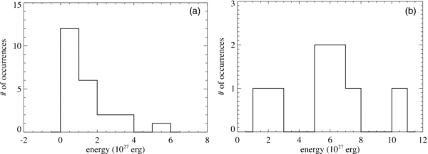
Figure 9. Energies calculated for loop shrinkage: (a) April 21 flare, (b) July 12 flare.
Download figure:
Standard image High-resolution image5. CONCLUSION
In a coarse description, "reconnection" means that a new magnetic connection is formed and an old connection abandoned. But the high conductivity of coronal plasma implies magnetic diffusion times much longer than the typical timescales of flares, so how can these new connections be allowed on timescales that are relevant? An answer that has been offered, paraphrasing Sweet (1958), Parker (1963), Petschek (1964), Jaggi (1964), and many others since, is that in a localized region resistivity may increase for a short time, so that reconnection can happen. But what exactly are the meanings of "localized" and "short time"? One must answer these questions to build a model of reconnection that can be compared with observations, or a model that actually predicts something. The observations discussed herein provide some tentative answers to these questions. Localization is addressed by the automated detection of SADs, providing the latitude, longitude, and a lower limit on the height. The duration of the reconnection episode may be related to the cross-sectional area of the outflowing flux tube (Linton & Longcope 2006).
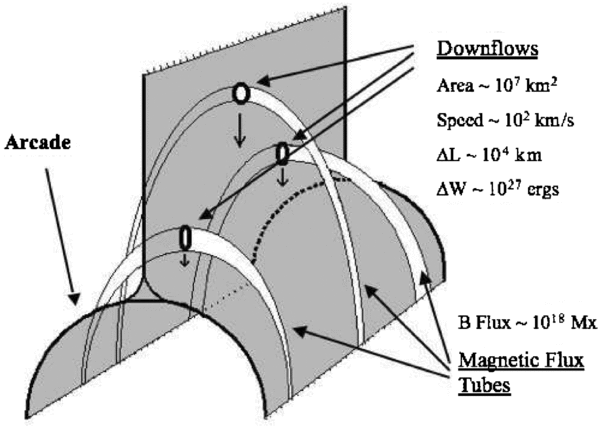
For SADs of the "plasma void" type in three flares observed by TRACE and SXT, we have derived empirical estimates of speeds, sizes, and included magnetic flux (see Figure 10). We believe these estimates, though model dependent, are potentially useful as inputs/constraints for models of three-dimensional reconnection. Measured cross-sectional areas are typically 107 km2, with significant range for variation. Plane-of-sky speeds range from approximately 30 to 260 km s−1, and are sub-Alfvénic. Combination of the SAD observations with magnetic modeling—in this case a PFSS model—yields an estimation of the flux in each shrinking flux tube. For two flares, the median flux in a shrinking tube is on the order of 1018 Mx. The energy associated with loop shrinkage appears to be of a significant magnitude; the present observations suggest ΔW ∼ 1027 erg per loop shrinkage, and reconnection rates on the order of 1016 Mx s−1. To our knowledge, these are the first empirical estimations of the flux participating in individual reconnection episodes, and of energy released by shrinkage, via measurements of postreconnection flux tubes. It is hoped that three-dimensional models of patchy reconnection will provide predicted distributions to which the observations can be compared.
Figure 10. Cartoon depiction of SADs resulting from patchy reconnection. Discrete flux tubes are created, which then individually shrink, dipolarizing to form the posteruption arcade. The measured quantities shown are averages from the current data set.
Download figure:
Standard image High-resolution image
This work was supported by NASA grant NNG04GB76G. The authors thank Drs. D. Longcope, M. Linton, and E. Priest for valuable discussions, and also to acknowledge the assistance of Mr. James Tolan and Ms. Letisha McLaughlin, participants in MSU's NSF-sponsored Research Experiences for Undergraduates (REU) program, NSF Award 0243923, during the summers of 2005 (JT), 2006 (LM), and 2007 (LM). The authors also acknowledge the comments of the anonymous reviewers.