


ABSTRACT
The classical picture of a star-forming filament is a near-equilibrium structure with its collapse dependent on its gravitational criticality. Recent observations have complicated this picture, revealing filaments to be a mess of apparently interacting subfilaments with transsonic internal velocity dispersions and mildly supersonic intra-subfilament dispersions. How structures like this form is unresolved. Here, we study the velocity structure of filamentary regions in a simulation of a turbulent molecular cloud. We present two main findings. First, the observed complex velocity features in filaments arise naturally in self-gravitating hydrodynamic simulations of turbulent clouds without the need for magnetic or other effects. Second, a region that is filamentary only in projection and is in fact made of spatially distinct features can display these same velocity characteristics. The fact that these disjoint structures can masquerade as coherent filaments in both projection and velocity diagnostics highlights the need to continue developing sophisticated filamentary analysis techniques for star formation observations.
Export citation and abstract BibTeX RIS
1. INTRODUCTION
Observations with the Herschel satellite have revealed that the backbone of molecular clouds is a compex network of connecting and interacting filaments (e.g., André et al. 2010; Molinari et al. 2010; Arzoumanian et al. 2011; Schneider et al. 2012). The dynamics of this web of dense molecular gas not only determines the evolution and stability of molecular clouds, but also regulates their condensation into stars. Molecular cloud cores and single low-mass stars are almost always found in filaments, often aligned like pearls on a string (Hartmann 2002; Lada et al. 2008; André et al. 2010). This can be interpreted as a result of the gravitational instability of a supercritical filamentary section (Inutsuka & Miyama 1997; Hacar & Tafalla 2011). Where filaments intersect, more massive hubs form (Myers 2009, 2013) that later could become the progenitors of star clusters.
Lada et al. (2010; see also, e.g., Enoch et al. 2007) demonstrated that the fraction of gas in the dense molecular web is of the order of 10% of the total molecular mass. Interestingly, the mass fraction of protostars to dense ( cm−3) molecular gas is also a constant on the same order. Burkert & Hartmann (2013) showed that this requires new filamentary segments to continuously form from the diffuse intra-filament medium on a gravitational collapse timescale.3
Classically, gas filaments have been treated as cylinders of gas in hydrostatic equilibrium (Ostriker 1964; Fischera & Martin 2012; Recchi et al. 2013). It is not clear, however, how such quiescent structures could form in the highly supersonic turbulent environment of a molecular cloud (e.g., Klessen & Hennebelle 2010; Heitsch 2013). In addition, millimeter line studies indicate that thermally subcritical filaments have transonic velocity dispersions while supercritical filaments can show super-thermal line widths, probably as a result of gravitational contraction (Arzoumanian et al. 2013).
More recently, observations by Hacar et al. (2013) revealed that filaments are often compact bundles of thin, spaghetti-like subfilaments. They presented observations of a prominent filamentary feature in Taurus dominated by the L1495 cloud (Lynds 1962) and several dark patches (Barnard 1927). They observed the region with the moderate density tracer C18O, obtaining spectra along a ∼10 pc length of the region. Analyzing the richest ∼3 pc section of the filament in the resultant position–position–velocity space, they found the intriguing result that the gas along the ridge is organized into velocity-coherent filamentary structures with typical lengths ∼0.5 pc. Each filament is internally subsonic or transsonic, although the collection of filaments is characterized by a mildly supersonic interfilamentary dispersion of ∼0.5 km s−1. They describe the collection of velocity detections as "elongated groups that lie at different "heights" (velocities) and present smooth and often oscillatory patterns." Multiple velocity components along a single line of sight have also been observed in Serpens South (Tanaka et al. 2013); this feature may therefore be common for many young star-forming sites.
The complexity of Hacar et al.'s position–position–velocity data, exemplified by their Figure 9, invites theoretical and numerical exploration. In particular, the apparent organization of filaments into bundles tends to bring to mind magnetic fields or other relatively complex physics. In this paper, however, we show that the bundle-like velocity signal is already present in simulated molecular clouds with a minimal set of physics, including just the interplay of gravity and hydrodynamic forces, acting on the initial turbulence.
2. THE SIMULATION
We simulated a 10 pc periodic cube of a molecular cloud, beginning from fully developed isothermal turbulent initial conditions. We generated the turbulent initial conditions using version 4.2 of the ATHENA code (Gardiner & Stone 2005, 2008; Stone et al. 2008; Stone & Gardiner 2009). The turbulent driving was technically similar to that of Lemaster & Stone (2009). Briefly, on a 10243 grid with a domain length of 1, we applied divergence-free velocity perturbations at every time step to an initially uniform medium. The perturbations had a Gaussian random distribution with a Fourier power spectrum  , for wavenumbers
  . Similar to, e.g., Federrath (2013), turbulence on smaller length scales was generated self-consistently from the large-scale driving.4
The driving continued until the box reached a saturated state at a Mach number
. Similar to, e.g., Federrath (2013), turbulence on smaller length scales was generated self-consistently from the large-scale driving.4
The driving continued until the box reached a saturated state at a Mach number  of roughly eight. During this driving stage, we did not include gravitational forces.
At this point, we scaled the box to a physical size S = 10 pc, mean number density n = 100 cm−3 at mean molecular weight  (giving a total gas mass ∼5700
  ), and a constant sound speed cs = 0.2 km s−1. After turning off forcing and turning on self gravity, we turned the simulation over to the adaptive mesh refinement code RAMSES (Teyssier 2002). The 10243 base grid was maintained and supplemented by four levels of adaptive refinement (maximum effective resolution 163843) triggered when the local Jeans length became shorter than 32 grid cells (Truelove et al. 1997; Federrath et al. 2011).
Regions violating the 32 cell Jeans length resolution limit on the finest level of refinement, and which are collapsing in all directions, were replaced by sink particles. For the cloud parameters, the density we use here is over an order of magnitude higher than the peak density generated by the turbulent driving, so that further checks such as those implemented by Federrath et al. (2010; for example, boundedness) are not necessary. The sinks accrete gas in a momentum-conserving fashion from a region that is 4 cells in radius (∼0.0024 pc) at the local Bondi–Hoyle rate in that region; sinks whose accretion zones touch are merged. The sinks are not the focus of this work and the sink implementation is fairly crude; due mainly to the simple equation of state and lack of radiative effects, they should not be thought of as simulated stars. Nonetheless, we can approximate the integrated star (rather, sink) formation efficiency as the fraction of the total mass in sinks at some time.
We integrated the box through ∼2.1 Myr of self-gravitating evolution. Following Kritsuk et al. (2007)'s definition of the turbulent turnover time in a box ,  , we have
  Myr. The free-fall time
 ![${T}_{\mathrm{ff}}={[3\pi /(32G\rho )]}^{1/2}$](https://content.cld.iop.org/journals/0004-637X/807/1/67/revision1/apj515476ieqn9.gif) at the mean density of the simulation is also roughly 3 Myr. In this paper, we focus on moderately dense gas with
at the mean density of the simulation is also roughly 3 Myr. In this paper, we focus on moderately dense gas with  ; at these densities, we have
  . After 1 Myr, the global structure of the simulated box is thus still dominated by the initial turbulence while the denser gas has had time to become organized by self gravity.
3. FILAMENT SELECTION AND ANALYSIS
After 1.27 and 2.09 Myr of self-gravitating evolution, we selected by eye filamentary segments in one projection of the cloud, shown in Figure 1. These images were constructed by calculating the surface density of gas in the range  . This is roughly the density range traced by C18O observations; we then converted the surface density to integrated line intensities. This conversion, using Equation (2) of Meier & Turner (2001), is only meant to give a low-order approximation to an observation. This approximate "observation" of our data yields an idea of what this simulation might look like in the motivating observations of Hacar et al. (2013). At 1.27 Myr, we chose one feature which, observationally speaking, would probably be deemed an obvious filament (filament D1), two that might be considered a ridge of star formation activity consisting of distinct dense sites linked by more tenuous emission (filaments B and C1), and one region that has entered a collapse phase (filament A). We stress that this is not intended to be a comprehensive study of all the filaments in this projection. In fact, it might be impossible to clearly identify individual filaments given the complex network of intersecting, elongated structures. Following Hacar et al. (2013), we therefore restricted ourselves to an exploratory look at a few of the more prominent filamentary segments. At this point, 26.7
  of gas is in sinks in filament A, yielding a global integrated sink formation efficiency of
  .
.
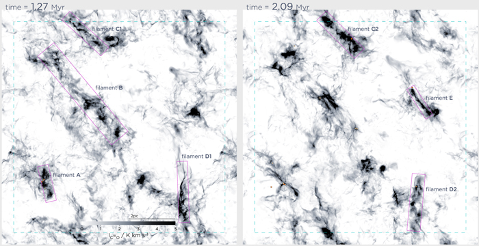
Figure 1. Surface density projections through the simulated volume at two times. The dashed cyan lines mark the boundary of the periodic simulation domain. We calculated the surface density using only the gas between  , and converted this to an approximation of an optically thin C18O observation. The magenta boxes delineate the filaments we focus on in this paper. Sink particles are shown as orange dots; note that although small in the image, the symbols are already 1.5 times larger than the size of the sinks in the simulation.
Download figure:
Standard image High-resolution imageAt 2.09 Myr, we selected three filamentary features. Two are evolved versions of the features at 1.27 Myr (filaments C2 and D2), while filament E formed in the intervening time. At this point, there are more sinks scattered through the box, including at least one in each of the filaments. The total sink mass is 121  , i.e., a global integrated sink formation efficiency
  .5
We chose to analyze these early times, before the gas has begun converting to sinks in earnest, to approximate the evolutionary state of Hacar et al.'s observations. The masses and dimensions of the sinks are summarized in Table 1.
.5
We chose to analyze these early times, before the gas has begun converting to sinks in earnest, to approximate the evolutionary state of Hacar et al.'s observations. The masses and dimensions of the sinks are summarized in Table 1.
Table 1. The Masses and Dimensions of the Filamentary Segments as Defined by the Boxes in Figure 1

|
Mgas |

|
L | W | ||
|---|---|---|---|---|---|---|
| Filament | sfe | |||||
( ) ) |
( ) ) |
( ) ) |
(pc) | (pc) | ||
| A | 52.7 | 121 | 26.7 | 0.18 | 1.7 | 0.51 |
| B | 192 | 550 | 0 | 0 | 5.5 | 1.0 |
| C1 | 67.3 | 159 | 0 | 0 | 2.5 | 0.55 |
| D1 | 70.9 | 143 | 0 | 0 | 2.9 | 0.5 |
| C2 | 130 | 244 | 5.38 | 0.022 | 2.5 | 0.65 |
| D2 | 68.0 | 159 | 7.15 | 0.043 | 2.7 | 0.60 |
| E | 37.7 | 77.5 | 2.75 | 0.034 | 1.7 | 0.40 |
Note.  is the moderate density mass contributing to that image; Mgas is the total gass mass;
  is the mass in sinks; sfe is the global sink formation efficiency in each filament,
  .
.
Download table as: ASCIITypeset image
3.1. Line-of-sight Velocity Structure
The rectangles surrounding the selected filaments define a coordinate system with axes aligned along the long axis or length L of the filament and the width W. The depth D is the same axis that the surface density is projected along. We stepped along the L and W coordinates with a stepsize equal to the simulation's base resolution, and calculated at each point the density-weighted line-of-sight velocity integrated along the D axis, using the same density range used to calculate the surface density. In more detail, each volume element in the simulation contributed a discrete line-of-sight velocity value. We converted these to Gaussian line profiles with dispersions of  km s−1, the thermal linewidth for C18O, with amplitudes proportional to the mass of material (in the appropriate density range) in the element, and binned these synthetic lines into histograms with bin width 0.05 km s−1.
In Figures 2 and 3, we show this data above the blowups of each filament. We summed the histograms along the W dimension, yielding the total velocity distribution along slices perpendicular to the filament's long axis. The character of the velocity distributions is surprisingly similar to the observations of Hacar et al. (2013); overlapping, linear, parsec-sized subfilaments with intrinsically subsonic line widths, combined into features with mildly supersonic dispersions. Note that we plot the raw density-weighted velocity structure rather than the centroids of line fits like those presented by Hacar et al. This accounts for the low-intensity background in the velocity plots. Nonetheless, arcs of higher intensity signal are clearly seen in our data.
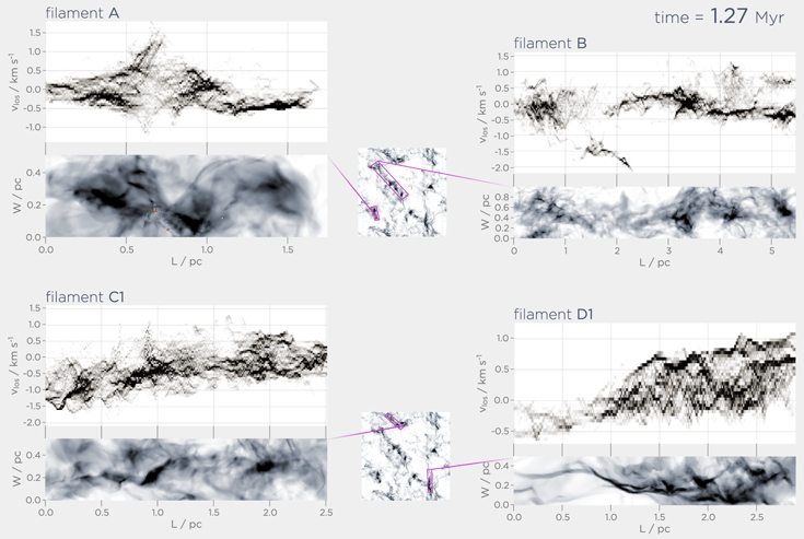
Figure 2. Filaments from the snapshot at 1.27 Myr, shown in their native coordinate system, along with line-of-sight velocity observations along the L dimension. These density-weighted line-of-sight velocities are summed along the W dimension, i.e., they are the L–v plane of the L–W–v position–position–velocity cube.
Download figure:
Standard image High-resolution image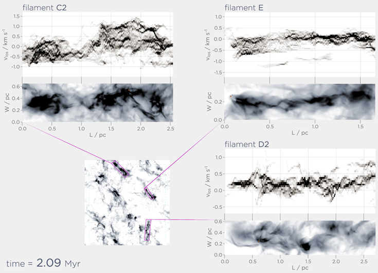
Figure 3. Filaments from the snapshot at 2.09 Myr, shown in their native coordinate system, along with line-of-sight velocity observations along the L dimension. These density-weighted line-of-sight velocities are summed along the W dimension, i.e., they are the L–v plane of the L–W–v position–position–velocity cube.
Download figure:
Standard image High-resolution imageThere are a few features in individual filaments worth mentioning. Filaments C1 and D1 show large-scale gradients of approximately 0.5 km s−1 pc−1 on top of which the ∼0.5 km s−1 dispersion is overlaid. The small-scale feature's velocity gradients are larger than the large scales', consistent with observations. Filament A's sink particles are clustered around L = 0.75 pc; the inflow of material to this small protocluster is clearly visible in the velocity plot while farther away from the clustering, the intertwining filaments in position–velocity space again show up. This same signal appears in filament D2 with about 7  of sinks at L = 0.6 pc. Filament B contains outlying material at a velocity of about −1.5 km s−1, quite distinct from the rest of the signal at mean velocities around 0 to −0.5 km s−1, a hint that some material in the ridge is only associated with the rest in projection. To further explore the coherence of the filaments, we turn to the 3D spatial extent of the selected regions at 1.27 Myr.
3.2. The Filaments' Third Spatial Dimension
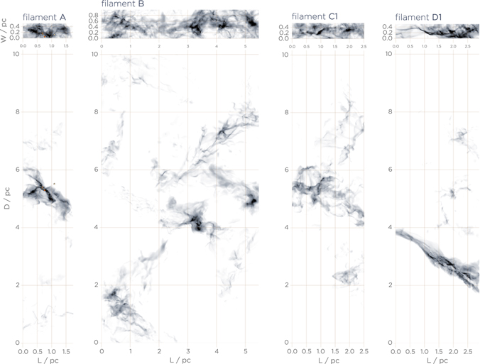
In Figure 4, we show the L–D projections along with the L–W projections from the left panel of Figure 1. Filaments A, C1, and D1 are revealed as spatially coherent entities along the projected axis with most of the material contained in a single connected distribution. Filament D1, in particular, is predominantly a 1D structure. Filament A, as the first site of sink particle formation in the simulated volume, is unsurprisingly compact in all three-dimensions. Filament B, in contrast, consists of distinct dense clumps, no closer to each other than about 2 pc, that are joined only in projection by more tenuous emission.
Figure 4. Third-dimension of the filamentary features from 1.27 Myr. The projections in the L–D plane show only the material that contributes to the surface density in the regions marked by the magenta boxes in the left panel of Figure 1, shown again here in the top panels.
Download figure:
Standard image High-resolution image
It is worth noting that there is nothing in the line-of-sight velocity information that obviously distinguishes filament B from C1 or D1. With the exception of the outlying material at  –2.25 pc, and
  to −2 km s−1 (which is the clump at
  –3.5 pc in Figure 4), the rest of the material appears to consist of distinct ribbons intertwining in position–velocity space with some large-scale gradients and a mildly supersonic dispersion.
4. CONCLUDING DISCUSSION
In this paper, we addressed the question of whether filamentary segments, identified by eye from a projected surface density map of a turbulent, self-gravitating cloud, when viewed in position–velocity space could reveal narrow, subsonic, elongated substructures moving transsonically with respect to each other, as discovered by Hacar et al. (2013). We therefore simulated a 10 pc region of a turbulent molecular cloud, allowing it to evolve under self gravity for 1.25 Myr. While the global structure of the region is still dominated by its turbulent structure, the denser gas has had time to become gravitationally organized.
No clear definition exists of how to define the boundaries of a filament. This might, in fact, be impossible in general as filaments are part of a complex network of elongated structures. We therefore treated our simulations as an observer might observe the sky, converting the density to an approximate line intensity and selecting by eye prominent filamentary segments. Many previous simulations of turbulent gas clouds have demonstrated the formation of long filamentary structures (e.g., Boldyrev et al. 2002; Federrath et al. 2010; Kritsuk et al. 2013). Here, we took the next step and studied their substructure in projected position–position–velocity space.
Our first main finding is that velocity characteristics very similar to those observed by Hacar et al. (2013) form naturally in such a turbulent setup. Individually gravitationally bound subfilaments display approximately sonic or subsonic dispersions and are organized in agglomerations of parsec-scaled larger filaments with transsonic to mildly supersonic relative motions. The large-scale velocity gradients are of the order of 0.5 km s−1 pc−1, while the small-scale features can have much larger gradients.
Second, the same velocity structures that appear in spatially coherent filaments can show up when observing a faux-filament. Based on the line-of-sight velocity information, there is not a clear case to be made that our filament B (particularly the section with  pc; see Figure 2) is different from filaments C1 or D1. Examining the third-dimension reveals it in fact to be composed of widely separated dense regions (Figure 4). Apparent velocity coherence similar to that seen in our most linear structures is evidently not enough to diagnose a true filament. The presence of this imposter filament in our data, not merely in projected density but also in the line-of-sight velocity, highlights the need for the continued development of sophisticated filament diagnostics, using both simulation and observation and both spatial and velocity data, in order to interpret not only existing observations of star-forming filaments but also the imminent (ongoing) onslaught of data from ALMA.
Is the bundle-like velocity structure just a relic of the imposed initial supersonic turbulence or the result of gravity working on a turbulent environment? In order to investigate this question, we ran a test simulation, starting with the same initial conditions, however, neglecting gravity. With the Mach number decreasing, the filaments got broader and did not form narrow, elongated structures as seen in the simulations with gravity. Subsonic, dense, spaghetti-like substructures are not seen in position–position–velocity space, indicating that the coordinating effects of gravity are important in their formation. We refer a detailed comparison of simulations with and without self gravity to a subsequent paper.
Further work using this simulation, and others like it exploring different boundary conditions and parameters, is in progress. These future efforts will quantify the qualitative agreement between the observed and simulated filaments, explore the time evolution of the simulated filaments, and utilize denser tracers (approximating N2H+) using the same algorithms as in Hacar et al. (2013).
We thank Alvaro Hacar and Jaoa Alves for motivating this research and interesting discussions, and the referee for many suggestions that improved the paper. This project has been funded by the priority program 1573 "Physics of the interstellar medium" of the German Science Foundation. Using yt (Turk et al. 2011)6 made analyzing the simulated data a great deal more efficient and painless than it otherwise would have been. N.M. sincerely thanks the development team for their rapid resolution of problems and squashing of bugs. In parts of this work, we made use of Astropy7 , a community-developed core Python package for Astronomy (Astropy Collaboration et al. 2013).
Footnotes
- 3
For context and alternative interpretations of this observation, see Padoan et al. (2014).
- 4
Note that the choice of solenoidal versus compressive driving can significantly alter the statistics and appearance of the turbulent structure (Federrath 2013). Beyond the scope of this paper, it would be interesting to see some of the many previous simulations of astrophysical turbulence that have been performed analyzed in the way presented here.
- 5
We note in passing that this efficiency is a factor of 1.4 lower than the most equivalent simulation of Federrath & Klessen (2012), within the expected scatter resulting from different turbulent seeds, box sizes, and densities.
- 6
- 7