


ABSTRACT
Based on the observed data by the Nobeyama Radio Observatory and the nonthermal gyrosynchrotron theory, the calculated magnetic field in a loop-like radio source of the 2001 October 23 flare attenuates from hundreds to tens of Gauss, except in the region with very weak magnetic fields. Meanwhile, the viewing angle between the magnetic field and line of sight has a similar attenuation from tens to around ten degrees, implying that the transverse magnetic component attenuates much faster than the longitudinal one. All of these results can be understood by the magnetic energy release process in solar flares. Moreover, the column density of nonthermal electrons decreases from 109−10 to 107−8 cm−2 during the flare, except in the region with very weak magnetic fields, where its value is larger than that with strong magnetic fields due to the mirroring effect. The calculated error and harmonic number of gyrofrequency better suit the region with strong magnetic fields.
Export citation and abstract BibTeX RIS
1. INTRODUCTION
Solar flares are generally considered to be the magnetic energy release process in the solar corona. Hence, the diagnostics of coronal magnetic fields is a key problem in solar flare physics. It is well known that the coronal magnetic field cannot be measured directly, as the solar photosphere is, and thus the extrapolated photospheric magnetic field is widely used to guess the coronal magnetic configuration and magnitude in solar flares. However, the variation of the photospheric magnetic field is mostly slower than that of solar flares. Flare-related changes of the photospheric magnetic field were reported, including an irreversible or permanent change observed during the pre- to post-phases of flares (e.g., Wang et al. 2012) and a transient or reversible change during the peak in the impulsive phase of flares (e.g., Maurya et al. 2012). Furthermore, some recent observations from the Solar Dynamics Observatory/Helioseismic and Magnetic Imager show that the photospheric magnetic transients possibly represent a real change in the magnetic field geometry (Harker & Pevtrov 2013; Kushwaha et al. 2014).
The variation of transverse magnetic energy becomes a hot topic in recent studies of photospheric magnetograms. For instance, Wang et al. (2012) provided a remarkably clear example of rapid flux emergence to show an increase in the transverse fields in the middle of the loop. The back reaction of Lorentz forces on the photosphere and solar interior may be caused by the coronal field evolution required to release flare energy resulting in the magnetic field of the photosphere becoming more horizontal (Hudson et al. 2008; Fisher et al. 2012; Wang & Liu 2010).
On the other hand, the radio diagnosis of coronal magnetic fields depends the observed radio flux or brightness temperature, which vary violently during the associated bursts. Based on the general expressions of gyrosynchrotron (GS) emission and absorption coefficients (Ginzburg & Syrovatskii 1965), the numerical calculations were applied for the nonthermal and mildly relativistic electrons in a homogeneous or dipole magnetic field (Ramaty 1969; Takakura & Scalise 1970). Some analytical approximations were proposed to fit the numerical results (Dulk et al. 1979; Petrosian 1981; Dulk & Marsh 1982). Especially, a group of analytical expressions over the range of harmonic numbers 10–100 of gyrofrequency, power-law index 2–7, and view angle 20°–80° are widely used to fit the strict GS theory (Dulk & Marsh 1982).
The nonthermal GS theory is the dominated mechanism of solar microwave bursts, thus it can be used for calculating the local magnetic field B of burst sources. Zhou & Karlický (1994) first deduced B and the column density of nonthermal electrons NL from two equations of optical thickness ( ) at the turnover frequency and radio flux in the optically thin region, based on the analytical approximations (Dulk & Marsh 1982), with the view angle θ as a free parameter. Afterwards, the equation of polarization degree from Dulk & Marsh (1982) was added to self-consistently obtain three solutions of B, NL, and θ (Huang 2006). Recently, a nonlinear equation of
  was derived from the above three equations, and a unique solution of
  θ may exist under a group of typical parameters in solar microwave bursts as shown in Figure 1 of Huang et al. (2013).
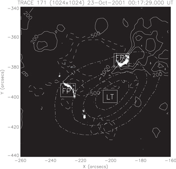
Figure 1. Two flare ribbons observed by TRACE 171Å at 00:17:29 UT of 2001 October 23 are overlaid by the SOHO/MDI positive (200, 600, and 800 Gauss) and negative (−500 and −1000 Gauss) contours, respectively, by solid and dashed lines, as well as by the dot–dashed contours of 17 GHz contours of brightness temperatures (1, 3, 5, and 7 × 10⁶ K) observed by the Nobeyama Radioheliograph (NoRH) around the peak time (00:16:50 UT) of this burst, while the magnetogram is about 17 minutes before the peak time of burst. The positions of one looptop (LT) and two footpoints (FP1 and FP2) are marked by white symbols and rectangles.
Download figure:
Standard image High-resolution imageMeanwhile, some flares were selected to test these methods, and fast variations of the coronal magnetic field were reported on the same timescales as associated bursts, even as fast as the magnetic reconnection. The formulae derived by Zhou & Karlický (1994) were used to calculate B and NL in the rising phase of one burst observed by the Owens Valley solar interferometer (Huang & Zhou 2000). The calculated B decreased with increasing radio flux in lower frequencies and increased with increasing frequency in the lower corona, the distribution of B became more homogeneous in different frequencies (or coronal heights). Moreover, NL increased with increasing radio flux in higher frequencies, and finally saturated, while some oscillations of NL appeared in lower frequencies. The spatially unresolved data of the Nobeyama Radio Spectrometers (NoRP) were analyzed in an X3.3 GOES-class flare on 1998 November 28 (Huang & Nakajima 2002; Huang 2006). The longitudinal magnetic field decreased very quickly from the initial time (several hundred Gauss) to the maximum (several ten Gauss), it remained in the low level during the impulsive phase and gradually returned to its original level in the decay phase, while the transverse magnetic component evidently did not change during the flare. The spatially resolvable data of NoRH in an M1.1 flare on 2004 November 1 were studied (Huang et al. 2008); the transverse magnetic component summed around the magnetic neutral line had a short-term impulsive increase during the rising phase, which may be considered as evidence of the magnetic reconnection in this flare.
However, the feasibility and accuracy for calculating the coronal magnetic field have not been fixed in the earlier papers, in most of which the authors paid attention to providing or improving the radio diagnostic method rather than analyzing the calculated coronal magnetic field in selected events. In this paper, the authors want to give a full and reliable description of one microwave burst with the results of radio diagnosis.
2. DATA SELECTION
A microwave burst associated with an M1.3 flare was selected from 24 loop-like events of the NoRH database (Huang & Nakajima 2009) for the radio diagnosis of coronal magnetic fields with some additional criterions for the data selection in this paper.
- 1.A strong and impulsive emission of more than 106 K is required in the flaring loops, including one looptop (LT) and two footpoints (FPs). The brightness temperature of the quiet Sun is about 104 K, and a criterion of 5 × 10⁴ K was used to select 24 loop-like events from NoRH for a statistical study by Huang & Nakajima (2009). However, the thermal free–free emission cannot be excluded in these events (Song et al. 2011); thus we take 106 K as a requirement to ensure that the nonthermal GS model is dominated in this study.
- 2.The burst source is closer to the solar disk center to verify the view angle between the magnetic field and line of sight (LOS) in a range of 20°–80°, which is required for the GS theory (Dulk & Marsh 1982).
- 3.The observed polarization sense with a positive sign is selected to assure the intrinsic mode of radio emission to be the extraordinary one in a positive magnetic polarity, which is also required by the GS theory (Dulk & Marsh 1982).
- 4.The peak or turnover frequency is mostly smaller than 10 GHz to ensure the working frequencies (17 and 34 GHz) of NoRH to be located in the optically thin part of nonthermal GS emission for calculating the spectral index properly in the observed microwave spectrum.
An interesting question to ask is how can you determine the exact locations of one LT and two FPs in the observed flaring loop with the lower spatially resolvable ability of NoRH (around 10 arcsec)? In the 2001 October 23 event, the radio image of NoRH shows the location of the LT source very well, but it is difficult to exactly locate the two FPs. In Figure 1, two flare ribbons observed by TRACE 171 Å in this event are overlaid by the MDI contours with opposite magnetic polarities and the 17 GHz contours of brightness temperatures observed by NoRH around the peak time of the burst. Hence, we can locate the FPs in two compact areas with strong EUV emissions, in which the TRACE image is about 40 s after the peak time of burst, while the MDI magnetogram is about 17 minutes before the peak time of the burst.
3. OBSERVATION
The time profiles of brightness temperatures at 17 and 34 GHz, the polarization degree at 17 GHz, and the spectral index calculated from the 17 and 34 GHz emissions are given in Figures 2(a)–(d), respectively. It is a complicated burst with multiple subpeaks of different timescales, so that a digital filter from the IDL routines was used to rule out some fast fluctuations and to recognize clearly the overall evolutions of observed and calculated parameters in Figure 2 and the following figures. The asymmetry is apparent in the two footpoint emissions; both the brightness temperature and polarization degree at 17 GHz in FP2 (dot–dashed line) are larger than those in FP1 (dashed line). The center of the radio source at 34 GHz seems to be deviated to the southeast of that at 17 GHz, while the radio loop is deviated to the southeast of the dipole magnetic field of the MDI as shown in Figure 3, probably caused by the projection effect. The positions of LT and FPs actually accord with the 17 GHz image, the 34 GHz data are only used to calculate the spectral index, and some error (±0.3) can be estimated by this deviation (Huang & Nakajima 2009).
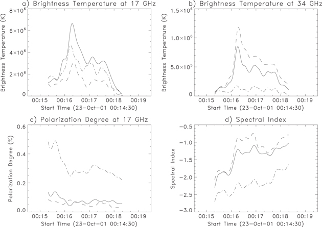
Figure 2. Time profiles of (a) brightness temperature of NoRH 17 GHz, (b) brightness temperature of NoRH 34 GHz, (c) polarization degree of 17 GHz, and (d) spectral index observed respectively in the looptop (solid) and the two footpoints (dashed and dot–dashed) of the 2001 October 23 flaring loop, in respect to the positions located in LT, FP1, and FP2 in Figure 1.
Download figure:
Standard image High-resolution image
Figure 3. (a) SOHO/MDI magnetogram about 17 minutes before the peak time of the 2001 October 23 flare overlaid by solid contours of the brightness temperature of NoRH 17 GHz (0.2, 0.4, 0.6, and 0.8 of its maximum) and dashed contours of the polarization degree at 17 GHz (0.01, 0.1, 0.2, and 0.3) around the peak time. (b) The brightness temperature of NoRH 17 GHz overlaid by solid contours of the brightness temperature of NoRH 34 GHz (0.2, 0.4, 0.6, and 0.8 of its maximum) and dashed contours of the minimum of equation of  (0.8, 1.0, 1.2, and 1.4) around the peak time. (c) The brightness temperature of NoRH 17 GHz overlaid by solid contours of the brightness temperature of NoRH 34 GHz (0.2, 0.4, 0.6, and 0.8 of its maximum) and the view angle (10°, 12°, and 14°) around the peak time. (d) The brightness temperature of NoRH 17 GHz overlaid by solid contours of the brightness temperature of NoRH 34 GHz (0.2, 0.4, 0.6, and 0.8 of its maximum) and dashed contours of the total magnetic field strength (0.1, 10.0, and 100.0 Gauss) around the peak time. The positions of one looptop (LT) and two footpoints (FP1 and FP2) in all the panels are given by Figure 1.
Download figure:
Standard image High-resolution imageMeanwhile, it was shown early on by two flares simultaneously observed by Yohkoh/HXT and NoRH (Kundu et al. 1995) that the strongest X-ray source had unpolarized radio emission; the strongest radio emission lay over a strong magnetic field and was polarized, but there was no coincident with the strongest HXR emission, which is consistent with a single and asymmetric loop model, as well as the observations in this event (see Figure 3(a)).
The data of NoRH at 17 and 34 GHz are not enough to determine the exact turnover frequency for the radio diagnosis in this paper; Figure 4 gives the time evolutions of the radio flux of NoRP at six frequencies, the typical microwave spectra at different phases of the burst, the spectral index of the optically thin part, and the turnover frequency, respectively, in which the turnover frequency is mostly below 10 GHz except in the maximum phase.
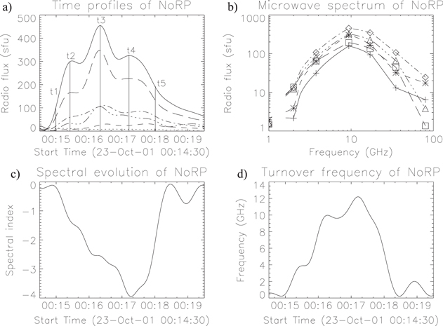
Figure 4. Time profiles of (a) the radio flux of NoRP at 1 GHz (dotted), 2 GHz (dashed), 3.75 GHz (dot–dashed), 9.375 GHz (solid), 17 GHz (long-dashed), and 35 GHz (dot–dot–dashed); (b) the spectra at t1 (solid and plus), t2 (dashed and asterisk), t3 (dot–dashed and diamond), t4 (dot–dot–dashed and triangle), and t5 (long-dashed and square); (c) the spectral index of the optically thin part; and (d) the turnover frequencies, respectively, in the 2001 October 23 flare.
Download figure:
Standard image High-resolution image4. RADIO DIAGNOSTICS
There are two equations derived in Huang (2006) for each the coronal magnetic field strength (B) and the angle (θ) between the the coronal magnetic field and the LOS based on the nonthermal GS formulae in Dulk & Marsh (1982):
and

where


Here, x =  and the electron gyrofrequency
  . All the coefficients in Equations (3)–(6) depend on five observable values, i.e., the radio observing frequency ν, the turnover frequency
  , the brightness temperature
  at a given frequency ν, the polarization degree rc, and the electron spectral index δ, which is calculated by
  , where α is the photon spectral index of the optically thin part (Dulk & Marsh 1982). Thus, it is easy to cancel out the terms with B in Equations (1) and (2) and to obtain a new equation of
  (Huang et al. 2013):
Therefore, the radio diagnosis in this paper can be performed in four steps as follows.
- 1.It is predicted that a unique solution of Equation (7) exists in the range of
 from 0 to 1 when θ is an acute angle under a group of typical parameters in solar microwave bursts, as shown by Figure 1 in Huang et al. (2013). Due to the limitation of approximations in Dulk & Marsh (1982), the accurate solution of Equation (7) may be sometimes absent, especially in a large range of the spatially resolvable data of NoRH, and it is difficult to evaluate the significance in this case. This problem is somehow solved after the equation of is derived in Huang et al. (2013), because we can always obtain the solution corresponding to the minimum of the left side of Equation (7) even when the observed data are beyond the theoretical limitation, and the calculated error can be roughly estimated by the minimum of the equation of . Therefore, the angle between the local magnetic field and the LOS is obtained in a broader range of observed parameters with a definite deviation from the accurate solution. The minimum values become smaller gradually in the burst source (Figure 3(b)), which just supports that the approximations of Dulk & Marsh (1982) are more acceptable inside the burst sources than outside.
 - 2.
- 3.The transverse and longitudinal components of coronal magnetic field are calculated, respectively, by and .
- 4.


Figure 3(c)–(d) shows the spatial distributions, respectively, of the calculated θ and B overlaid on the peak-time images of the brightness temperature at 17 GHz, with the solid contours of the brightness temperature at 34 GHz. Both θ and B gradually increase from FP1 to the LT and FP2 sources; such a tendency is also clearly seen in the time evolutions of θ and B in the three sources (Figure 5(b)–(c)), as well as the transverse and longitudinal magnetic components (Figure 6(a)–(b)).
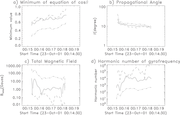
Figure 5. Time profiles of (a) the minimum value of equation of  , (b) the view angle θ, (c) the total magnetic field B, and (d) the harmonic number of gyrofrequency calculated in the looptop (solid) and the two footpoints (dashed and dot–dashed) of the 2001 October 23 flaring loop, with respect to the positions located in LT, FP1, and FP2 in Figure 1.
Download figure:
Standard image High-resolution image
Figure 6. Time profiles of (a) the transverse magnetic field, (b) the longitudinal magnetic field, (c) the ratio of the transverse and longitudinal magnetic components, and (d) the column density of nonthermal electrons calculated in the looptop (solid) and the two footpoints (dashed and dot–dashed) of the 2001 October 23 flaring loop, with respect to the positions located in LT, FP1, and FP2 in Figure 1.
Download figure:
Standard image High-resolution image
The most important evolutionary behavior of B is that it decreases rapidly from the start time to the maximum time of burst and keeps low strength until the decay phase and the total variation is up to one order of magnitude (from hundreds to tens Gauss), but this attenuation evidently does not appear in the FP1 source (dashed line in Figure 5(c)) with very weak magnetic fields (less than 1 Gauss). Meanwhile, a similar attenuation of θ appears in the three sources from tens to about ten degrees, and due to the similar behavior of θ and B, the attenuation of the transverse magnetic component is more apparent than that of the longitudinal one, which is clearly shown by the ratio between the transverse and longitudinal magnetic components in Figure 6(c). It is a little unexpected that NL also decreases from 109−10 to 107−8 cm−2 during the flare, which is more evidently seen in the FP2 source (dot–dashed line in Figure 6(d)), while NL roughly decreases from the FP1 to the LT and FP2 sources, which seems to be opposite to the variations of θ and B in the three sources.
5. DISCUSSIONS AND CONCLUSIONS
Based on the magnetic energy release process in solar flares, it is not difficult to understand such an attenuation of the calculated magnetic field in a flaring loop. We can directly predict that the coronal magnetic field is inversely proportional to the brightness temperature or radio flux of solar microwave bursts from an analytical expression (Equation (9)) in Zhou & Karlický (1994) when the other parameters do not change much, as well as from some earlier calculations, such as Figure 6 in Huang (2006). Therefore, this is probably a common behavior of coronal magnetic fields in solar flares. Even the time evolution of the total magnetic field and view angle (Huang & Nakajima 2002; Huang 2006) is somehow similar to that in this paper, but their enhancement during the decay phase does not appear in the event of this paper, hence the coronal magnetic attenuation is an irreversible or permanent change for this event under investigation.
Moreover, the transverse magnetic attenuation in a flaring loop is more evident than that of longitudinal component due to the similar behavior of the total magnetic field and view angle, which is also consistent with our knowledge about the dependence of flare energy mainly on the transverse magnetic energy, as well as the recent studies about the magnetic field of the photosphere becoming more horizontal during flares (Hudson et al. 2008).
The variation of the propagation angle from tens to about ten degrees during the rising phase is suggested in this event as well as in the two events of earlier papers (Huang 2006; Huang et al. 2008). The variation of angle indicates the change of the overall magnetic configuration during flares. Thus, we can use it to probe the magnetic shear changes of the coronal magnetic field; a fast relaxation process of a sheared coronal magnetic field was reported by Ji et al. (2006), and the relaxation is believed to be a shrinking process. The decrease of the angle by radio diagnosis may provide additional evidence for the relaxation process.
Regarding the strong asymmetry of the calculated magnetic field and column density up to one or two orders of magnitude in the flaring loop, an analytic model was proposed for an asymmetric magnetic flux tube to determine the ratio of the precipitating rates and the asymmetric radio and hard X-ray emissions at two feet of a flux tube (Melrose & White 1979, 1981), that is not only caused by different mirror ratios but also caused by different initial pitch angles at two feet as shown in a recent statistics of 24 flaring loops observed by NoRH (Huang et al. 2010). The disconnected points that appeared in the time evolution of the column densities in the LT and FP1 (see Figure 6(d)) result from the data overrun interrupt. The mirroring effect can be used to explain why a stronger magnetic field and smaller column density appear in FP2, while a weaker magnetic field and larger column density exist in FP1 and LT, as shown in Figures 5 and 6. It also helps us understand why the polarization degree in FP2 is evidently larger than that in FP1 and LT (Figure 2(c)) due to the dependence of the polarization degree on the local magnetic field strength (see Equation (16) of Dulk & Marsh 1982). However, the 17 GHz brightness temperatures in FP2 are a little higher than those in FP1 (Figure 2(a)), while the 34 GHz brightness temperatures in FP2 are one order of magnitude lower than those in FP1 (Figure 2(b)), which is more complicated than that in Kundu et al. (1995), and is possibly caused by the projection effect.
The method for calculating the coronal magnetic field and electron column density strongly depends on the approximations in Dulk & Marsh (1982), which should be performed strictly under the conditions of  and 10 ≤ S ≤ 100 (S is the harmonic number of gyrofrequency), with the propagation angle
  . The peak frequency is roughly defined as the frequency at the optical depth
  , the low cut-off energy E0 = 10 keV, and the emission being dominated by the X-mode. Also, these approximations can only be used for a simple and isolated source without significant changes in the magnetic field, the angle, or other quantities, along the LOS within the emission region. In the given ranges of the harmonic number, electron energy spectral index, and viewing angle, the error in the approximations of Dulk & Marsh (1982) is less than 30% with respect to the full expressions of GS emission (Takakura & Scalise 1970), but the accuracy worsens at δ > 6, especially, at the extremes of θ and S (Dulk 1985).
The minimum of equation of  is used to evaluate the calculated error in this paper, which depends on the deviation of the nonthermal GS model from the observed events. We may check with Figure 5(a) that the minimum of the equation of
  in FP2 (dot–dashed line) with a stronger magnetic field is evidently smaller than that in LT (solid line) and FP1 (dashed line) with weaker magnetic fields (also see Figure 3(b)), because the nonthermal GS theory is not enough to cover all radiation processes, such as the thermal bremsstrahlung mechanism in the radio source with very weak magnetic fields. A theoretical error (26%) was given by Dulk & Marsh (1982) under the approximated conditions, but this error will increase rapidly beyond those conditions. In this paper, we can roughly estimate the error by the minimum of the equation of
  (Figure 5(a)) with respect to the analytical approximations of Dulk & Marsh (1982), for instance, the error is 20%–40% in the footpoint with a strong magnetic field (under the conditions) and 60%–80% in the LT and footpoint with weak magnetic fields (beyond the conditions), which should be added to the magnitude of error analysis in Dulk & Marsh (1982).
We can also check the harmonic numbers in the three sources (Figure 5(d)), and find that the harmonic number is smaller than 100 only in FP2 (dot–dashed line), which is suitable for the GS theory of Dulk & Marsh (1982). In fact, a full GS spectrum is predicted by the GS theory in a uniform magnetic field (Ramaty 1969), which means that the GS emission at a given frequency is actually determined by an integration of different harmonics of gyrofrequency in a nonuniform magnetic field, such as a dipole (Takakura & Scalise 1970). Hence, the harmonic number obtained in this paper can be approximately considered to be its mean value in a nonuniform magnetic field, which is useful for estimating the mean height of radio source at a given frequency above the photosphere.
There are some other problems with the present radio diagnosis; one is a 180° ambiguity of the calculated θ due to different definitions of polarizations in theory and observation (Huang et al. 2013), but this does not affect the main conclusions with small view angles in this paper. Another problem is caused by a rough spectral resolution of NoRH and NoRP to obtain the spectral index and turnover frequency, which may be solved after a new radioheliograph working at multiple frequencies is established in the world (Yan et al. 2012).
The study is supported by the NFSC project Nos. 11333009, 11073058, 11273030, 11373039, 11203083, and 41331068, the "973" program Nos. 2011CB811402 and 2011CB811401. The authors would like to thank the NoRH, MDI, and TRACE teams for data preparing and preprocessing.