


ABSTRACT
We study how the magnetorotational instability (MRI) in protoplanetary disks is affected by the electric discharge caused by the electric field in the resistive magnetohydrodynamic. We performed three-dimensional shearing box simulations with various values of plasma beta and electrical breakdown models. We find that the MRI is self-sustaining in spite of the high resistivity. The instability gives rise to the large electric field that causes the electrical breakdown, and the breakdown maintains the high degree of ionization required for the instability. The condition for this self-sustained MRI is set by the balance between the energy supply from the shearing motion and the energy consumed by ohmic dissipation. We apply the condition to various disk models and study where the active, self-sustained, and dead zones of MRI are located. In the fiducial minimum-mass solar-nebula model, the newly found sustained zone occupies only a limited volume of the disk. In the late-phase gas-depleted disk models, however, the sustained zone occupies a larger volume of the disk.
Export citation and abstract BibTeX RIS
1. INTRODUCTION
Protoplanetary disks are the sites of planet formation. Disk turbulence greatly affects the mutual sticking of the planetesimals and their settlement to the disk midplane. The turbulence is the source of angular momentum transfer in the disk that causes gas accretion and migration of the planetesimal onto the central star. Thus, understanding the evolution of the turbulence within protoplanetary disks is an essential step in studies of both disk evolution and planet formation.
Magnetorotational instability (MRI) is considered to be the major source of turbulence in many types of accretion disks, including protoplanetary disks (Balbus & Hawley 1998 and references therein). One of the distinct properties of protoplanetary disks compared to other accretion disks is that the major parts of protoplanetary disks are only weakly ionized and the magnetic diffusivity affects the MRI (Sano et al. 1998; Fleming et al. 2000). The low ionization degree is due to their low temperature and high number density of the dust component.
In protoplanetary disks, the MRI and dust components affect each other. The turbulence is one of the sources for the relative velocities of colliding dust (Ormel & Cuzzi 2007; Brauer et al. 2008) and contributes both to dust growth and disruption (Blum & Wurm 2008; Wada et al. 2008; Güttler et al. 2010; Wettlaufer 2010). On the other hand, dust particles in protoplanetary disks are the major sites of charged particle recombination, and thereby influence the ionization degree of the disk (Sodha et al. 2009; Umebayashi & Nakano 2009; Grach et al. 2010).
The dead zone can occupy a large volume of a protoplanetary disk, especially in the presence of abundant small dust grains (Gammie 1996; Sano et al. 2000; Ilgner & Nelson 2006). However, various electric discharge mechanisms in protoplanetary disks have been proposed (Horanyi et al. 1995; Desch & Cuzzi 2000; Muranushi 2010) that may provide a higher ionization degree compared to the values predicted by the dust-absorption equilibrium models, resulting in the increased MRI activity in the disk. They consider the electron avalanche process, an exponential growth in the number of conducting electrons that takes place when the kinetic energy of the electrons exceeds the ionization energy of a neutral gas molecule. The result is electrostatic breakdown, the lowering of the resistivity of the fluid and electric discharge, and an increase of the electric current through the fluid.
Moreover, a model has been proposed where the MRI itself provides sufficient ionization (Inutsuka & Sano 2005, hereafter IS05). IS05 have shown that that the electric field typically generated by protoplanetary disk turbulence is strong enough to drive the electrons away from the thermal Maxwell–Boltzmann distribution. Those energetic electrons contained in the electric current cause the electric discharge and maintain the ionization degree high enough for the MRI to survive. IS05 have also shown that the energy supply from the shearing motion is about 30 times larger than the energy required to maintain a sufficient number of electrons in the presence of standard dust grains.
However, IS05 have studied only one-zone models, and with only one set of parameters typical to 1 AU of the disk. In this work, we extend the model IS05 to a local, three-dimensional simulation of protoplanetary disks and study the interaction of the MRI with the discharge ionization. We also apply the model to global models of protoplanetary disks and study where and when in the disk the self-sustainment of MRI takes place.
This paper is organized as follows: In Section 2, we perform the numerical simulations of the MRI in unstratified, three-dimensional shearing-boxes along the lines of Hawley et al. (1995, hereafter HGB95) with the nonlinear ohmic diffusivity added. In Section 3, we analyze the activity of the MRI in the protoplanetary disk, using the method of Sano et al. (2000, hereafter SMUN00). To calculate the ionization degree in the disk we use the method proposed by Okuzumi (2009, hereafter O09). Section 4 is devoted to conclusions and discussions. Table 1 lists the symbols frequently used in this paper.
Table 1. List of Symbols Used in This Paper
| Symbol | Value | Definition | Location |
|---|---|---|---|
| (Dimension) | |||
| ρ | (g cm−3) | Gas density | (4) |
 |
(cm s−1) | Gas velocity | (5) |
 |
(g1/2 cm−1/2 s−1) | Magnetic field | (6) |
| P | c2sρ | Pressure with isothermal equation of state | (7) |
| E | (g1/2 cm−1/2 s−1) | Electric field in the lab frame | (8) |
| E' | (g1/2 cm−1/2 s−1) | Electric field in the comoving frame | (1) |
| J | (g1/2 cm−3/2 s−1) | Electric current | (9) |
| η0 | (cm2 s−1) | Linear coefficient and — | |
| Jcrit | (g1/2 cm−3/2 s−1) | — critical current for extended Ohm's law | (2) |
| P0 | (g cm−1s−2) | Initial pressure | |
| β | 2c2s/vAZ2 | Plasma beta | |
| Bz0 |  |
Initial, vertical net magnetic field | (15) |
| H | cs/Ω | Disk scale height | (14) |
| Beqp |  |
The nondimensionalization unit of magnetic field | (12) |
| Jeqp | cBeqp/4πH | The nondimensionalization unit of current | (13) |
| RM |  |
Magnetic Reynolds number | Section 2.2 |
 |
1.0 | Surface density multiplier | (37) |
| q | 3/2 | Power-law index of the surface density | (37) |
| ad | 0.1 μ m | Radius of solid dust particle | (44) |
| fd | 0.01 | Dust-to-gas ratio | (47) |
Download table as: ASCIITypeset image
2. SIMULATIONS OF THE MRI WITH NONLINEAR OHM's LAW
2.1. Numerical Setup
There are three diffusion terms in magnetohydrodynamic (MHD); they are ohmic diffusion, Hall diffusion, and ambipolar diffusion. In protoplanetary disks, any one of the three modes can be the dominant mode depending on dust and gas density (e.g., Wardle 2007), and interaction between the different modes may alter the MRI (Wardle & Salmeron 2012). In this paper, we only focus on the ohmic diffusion because it is the most studied one in the context of the MRI. We leave the treatment of other diffusion modes for future studies.
The electric discharge taken into account, we construct a simple model of the discharge as follows, in terms of an appropriate η0 and Jcrit:
and
This nonlinear diffusivity model states that the electric field on the fluid comoving frame never exceeds a critical value, E'crit = 4πc−2η0Jcrit, and thus the magnetic diffusivity η varies depending on electric current J, and Ohm's law become nonlinear.
Note that the smallest space scale dealt with in this paper is on the order of 10−2 AU. The actual scale of the discharge structures can be much smaller than this. The estimate for the lower limit of the size of such structures is their thickness, which is on the order of 5000 times the electron mean free path (Pilipp et al. 1992).
However, we can derive the macroscopic discharge model from the microscopic discharge relation |E'| < E'crit that holds everywhere in the plasma. Since, e.g., the x-component of the discretized electric field 〈E'x〉 is obtained from the line integral of the real field over the discretization length ΔV,
Therefore, we can use Equations (1) and (2) as a "coarse-grained model" where we can interpret E' and J as spatial averages. If electrical breakdown occurs in a scale smaller than the grid size, the spatially averaged electric field is smaller than E'crit. Thus, in general, the electrical breakdown may occur even in the region where 〈E'crit〉 is smaller than E'crit. Therefore, if we adopt Equations (1) and (2), we may underestimate, but not overestimate, the occurrence of electric discharges.
We adopted a local, Kepler-rotation shearing box that has radial (x), azimuthal (y), and vertical (z) axes and solved the following resistive MHD equations numerically:
with isothermal equation of state (EOS)

Had we used the adiabatic EOS, the internal energy would have kept growing as the linear function of time (HGB95). Therefore, we use the isothermal EOS to approximate the steady state attained by the cooling processes present in the protoplanetary disks.
The nonlinear Ohm's law reads:
Here, we have studied three different models for nonlinear diffusivity η(J). In addition to our fiducial model (fid), Equations (1) and (2), we have studied the following two models:
and
The electric field as a function of current density in these three models is shown in Figure 1.
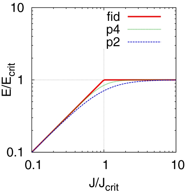
Figure 1. Electric field amplitude as functions of current in the three different models of nonlinear Ohm's law. The symbols fid, p2, and p4 correspond to Equations (2), (10), and (11), respectively.
Download figure:
Standard image High-resolution imageFollowing HGB95, we set up our numerical initial conditions as follows. We use the disk scale height H as the unit length. The box size is (Lx, Ly, Lz) = (1, 2π, 1). First,we set the average values ρ0 = 1 and P0 = 10−6 to every mesh and let fluid velocity be at rest in the shearing box frame; (vx, vy, vz = 0, −(3/2)Ωx, 0). Here, cs = 10−3, and also Ω = 10−3.
Next, we introduce random perturbations in density, pressure, and velocity. The density and pressure perturbations are in proportion so that the isothermal EOS is met, and the amplitude is δρ/ρ0 = δP/P0 = 2.5 × 10⁻². We perturb the velocity componentwise, with the amplitude δvi = 5 × 10⁻³cs for each.
We use the following units for the magnetic field, electric current, and scale height, respectively:

and
We set the uniform magnetic field in the z-direction and express the initial field strength by the plasma beta,

The plasma beta satisfy the following relation between the sound speed cs and the Alfvén velocity along the magnetic field  :
:
We define the magnetic Reynolds number as

using the Alfvén velocity  set by the initial vertical magnetic field. This is in accordance with SMUN00 and IS05, though some literature adopts a different definition (e.g., RM ≡ cs2/η0Ω in Fleming et al. 2000).
We have used Athena (Gardiner & Stone 2005, 2008), an open-source MHD code, for our simulations.
2.2. Simulations Procedure
We vary the initial magnetic field strength and the diffusivity models and we classify each set of parameters as either ◯active zone, ×dead zone, or ▵sustained zone. The experiment method and the definition of the three classes are given in this section.
The parameters we have investigated are the initial vertical field strength (represented by plasma β), the linear diffusivity (represented by magnetic Reynolds number RM), and the critical current Jcrit. The range of the survey was 400 ⩽ β ⩽ 25600, 0.002 ⩽ RM ⩽ 2, and 0.01 ⩽ Jcrit/Jeqp ⩽ 100. In addition, the limiting cases of RM = ∞ and Jcrit/Jeqp = ∞, which correspond to ideal MHD models and linear Ohm's law models, respectively, are studied for comparison with the literature.
For each value of β, we prepared the initial condition as described in Section 2.1 and continued the simulation for 10 orbits (t = 20π/Ω), at first with magnetic diffusivity turned off (η(J) = 0). While running the simulations, we created restart data for each periodic point (t = 2nπ/Ω, where n is an integer). The condition allowed the MRI to grow and saturate in about 5 orbits (t = 10π/Ω).
Then, for each pair of (RM, Jcrit/Jeqp), we turned on the diffusivity and restarted the simulation either from the initial laminar flow (t = 0) or the saturated MRI states at 8, 9, and 10 orbits (t = 16π/Ω, 18π/Ω, 20π/Ω). We numerically evolved them until they reach 20 orbits (t = 40π/Ω). The reason why we have adopted three different MRI saturated initial conditions (t = 16π/Ω, 18π/Ω, 20π/Ω) for each set of the parameters is that a "turbulent initial condition" is not unique, and therefore we need to test if our results depend on the choice of the initial condition or not.
During each simulation run, we recorded the space averages of physical quantities as functions of time, such as magnetic energy density B2, the Reynolds and Maxwell stress ρvxδvy, −BxBy/4π, and the squared current J2. After the simulations, we studied the time average of the quantities. For a physical quantity A, we denote its space and time average by 〈A〉 and  , respectively. Their definitions are as follows:
and
The space average is taken for the entire computational domain (0 < x < Lx, 0 < y < Ly, 0 < z < Lz), the numerical resolution is (Nx, Ny, Nz) = (64, 128, 64), and the time average is taken for the last five orbits (30π < t < 40π) unless otherwise mentioned. Statistics for the important sets of parameters are presented at the end of the paper.
Using the average values, we classify each set of the parameter (β, RM, Jcrit/Jeqp) as follows (cf. Table 2): First, a parameter is in ◯active zone if the MRI is observed both in the simulation started from the laminar flow as well as in all of the three simulations started from the saturated MRI states. Second, a parameter is in ×dead zone if the instability is observed neither in the simulation started from the laminar flow nor in any of the three simulations started from the saturated MRI states. Finally, a parameter is in ▵sustained zone if the MRI is observed in all the three simulations started from the saturated MRI states, but not at the end of the simulation started from the laminar flow.
Table 2. Zone Names and Meaning of the Symbols in Figures 3 and 4
| Zone | From Laminar? | From Ideal MRI? |
|---|---|---|
| ◯active | Unstable | Unstable |
| ×dead | Stable | Stable |
| ▵sustained | Stable | Unstable |
Download table as: ASCIITypeset image
2.3. Result of Shearing-box Simulations
The typical behavior of the current for the active zone, dead zone, and sustained zone is in Figure 2. From the simulations, we have observed that the three classes (active, dead, and sustained) are exhaustive: the runs started from 8, 9, and 10 orbits always agree in terms of the classification and if the MRI dies when starting from a saturated initial condition, it also does not activate starting from a laminar initial condition.
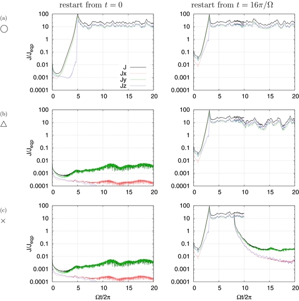
Figure 2. Time evolution of the averaged current density for three magnetic diffusivity models. The models are (a) β = 400, RM = 0.6, Jcrit/Jeqp = 1, (b) β = 400, RM = 0.2, Jcrit/Jeqp = 1, and (c) β = 400, RM = 0.2, Jcrit/Jeqp = 10. The graphs show typical current behavior for (a) ◯ active zone, (b) ▵ sustained zone, or (c) × dead zone.
Download figure:
Standard image High-resolution imageTo classify the active, dead, and sustained zones, we need to assess the magnetorotational instability of the system, so we introduce the criteria below for quantitative assessment. We say that the system is magnetorotationally unstable if the averaged current 〈J2〉1/2 is greater than 0.1Jeqp, and stable if otherwise. Here, the time average is taken for the last five orbits (30π < t < 40π). We have learned from the simulations that the quantity 〈J2〉1/2 is a good indicator of stability, since it either fluctuates around the mean value 〈J2〉1/2 ≃ 10Jeqp (unstable) or goes under 〈J2〉1/2 < 0.1Jeqp almost monotonically with little vibration (stable). There is no ambiguity between the two (cf. Figure 2).
However, as we make RM smaller, the diffusion timescale becomes shorter and the wall clock time for the simulations until t = 40π becomes impractically larger. Therefore, for the parameter range RM < 0.01, we terminate the simulations at 1.5 × 10⁶ cycles and determine the class by extrapolations.
Figures 3 and 4 show the result of our parameter survey. We found that sustained zones exist—the MRI does exhibit hysteresis behavior for a certain set of parameters.
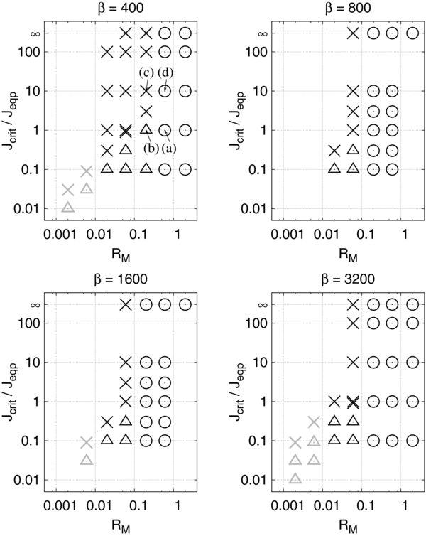
Figure 3. Distribution of the sets of parameters (β, RM, Jcrit/Jeqp) in our simulations. We classify each of them as either ◯ active zone, ▵ sustained zone, or × dead zone. This page includes the data for 400 ⩽ β ⩽ 3200. The parameters classified by extrapolations are marked by light gray symbols.
Download figure:
Standard image High-resolution image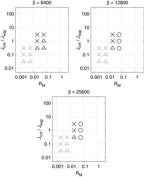
Figure 4. Continued from Figure 3, the data for 6400 ⩽ β ⩽ 25600.
Download figure:
Standard image High-resolution imageTo study possible influences of the numerical resolutions, we have performed simulations using the different numerical resolutions Nx = 32, 48, 64, (fiducial) and 80 while keeping the aspect ratio Nx: Ny: Nz = 1: 2: 1, for three different sets of parameters (β, RM, Jcrit/Jeqp) = (400,0.6,1), (400,0.2,1), and (400,0.2,1). Figure 5 summarizes the convergence tests. Within these sets of parameters, we observe that our classification does not depend on the numerical resolution.
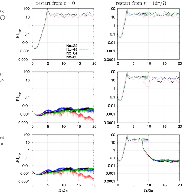
Figure 5. Dependence of the MRI behavior on the resolution. The development of electric current over time in the simulations using the different numerical resolutions Nx = 32, 48, 64 (fiducial), and 80 while keeping the aspect ratio Nx: Ny: Nz = 1: 2: 1, for three different sets of parameters (a) β = 400, RM = 0.6, Jcrit/Jeqp = 1, (b) β = 400, RM = 0.2, Jcrit/Jeqp = 1, and (c) β = 400, RM = 0.2, Jcrit/Jeqp = 10. These are typical parameter sets for (a) ◯ active zone, (b) ▵ sustained zone, and (c) × dead zone, respectively.
Download figure:
Standard image High-resolution imageWe also studied if our result depends on the model of the nonlinear Ohm's law. In addition to our fiducial (fid) model (Equation (2)), we have studied two smoothly transiting models (Equations (10) and (11)). To distinguish the three models, see Figure 1.
Figure 6 summarizes the time evolution of the current density in the simulations with the three typical sets of parameters (β, RM, Jcrit/Jeqp) = (400,0.6,1), (400,0.2,1), and (400,0.2,1). Within the regime we have tested, the hysteresis behavior does not depend on the detail of the nonlinear resistivity models.
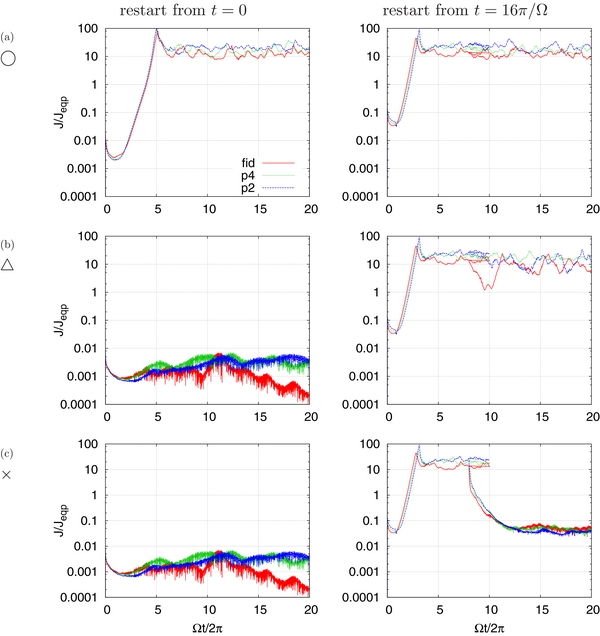
Figure 6. Dependence of the MRI behavior on resistivity models. The development of electric current over time in the simulations using different resistivity models fid (Equations (1) and (2)), p2 (Equation (10)), and p4 (Equation (11)), for three sets of parameters (a) β = 400, RM = 0.6, Jcrit/Jeqp = 1, (b) β = 400, RM = 0.2, Jcrit/Jeqp = 1, and (c) β = 400, RM = 0.2, Jcrit/Jeqp = 10, which are typical parameter sets for (a) ◯ active zone, (b) ▵ sustained zone, and (c) × dead zone, respectively.
Download figure:
Standard image High-resolution imageFrom Figures 3 and 4, we can see the following condition for the ▵sustained zone:
where fwhb is a proportionality constant that satisfies fwhb ≃ 5–15 for 400 ⩽ β ⩽ 1600, and fwhb ≃ 15–50 for β ⩾ 3200. Hereafter, we interpret this in terms of the work-heat balance in the resistive MRI.
We also remark that within parameter regions that is in active zone, RM < 1, and with larger Jcrit, we observed the large-amplitude time-variability of physical quantities, such as magnetic fields, due to repeated growth and reconnection of the channel solutions. This phenomenon is reported by Fleming et al. (2000).
2.4. Interpretation of the Simulation Results
In this section, we show that Equation (20) can be understood as a condition of the balance between the magnetic energy dissipated by Joule heating per unit volume (WJ) and the work done by shearing motion per unit volume (Wsh).
Let us define Qwhb as the left-hand side of Equation (20):
The condition for self-sustained MRI is Qwhb < fwhb, which will be explained in this section.
First, substitute  :
:
Next, when the MRI is active, 〈J2〉1/2 ≃ fsatJeqp where fsat is of the order of 10. Since this average current strength lies in the super-critical regime of Ohm's law (J > Jcrit), the electric field is E'crit = 4πc−2η0Jcrit as modeled in Equations (1) and (2). Therefore, the Joule heating per unit volume is estimated to be
To explain the work-heat balance qualitatively, this estimate needs correction due to the high space variability of the current field under the discharge conditions. We introduce ffill, or the filling factor, which is the ratio of the volume that contributes to the Joule heating to the total volume. Formally, ffill is defined as the ratio between volume averages of the actual Joule heat generated and the Joule heat estimated by this method:

where
Using this ffill, Equation (23) is rewritten as

Substituting η0 in Equation (22) with Equation (26) gives
Substituting  with Equation (16) and then cs with Equation (14), Jeqp with Equation (13) and then Beqp with Equation (12) gives
On the other hand,
where α is Shakura & Sunyaev's (1973) α parameter. Substituting Equation (29) into Equation (28), one obtains
For the MRI to sustain itself by the discharge process, the Joule heating WJ needs to be equal to or smaller than Wsh:

Therefore, we have the following constraint on the left-hand side of Equation (22):
Thus, the work-heat balance imposes an upper limit on the product of Jcrit/Jeqp and 1/RM, provided that ffill, fsat, and α are constants that do not depend on Jcrit and RM, but only on β. This explains the inverse-proportional relations observed in Figures 3 and 4. The fwhb(β) values calculated with this interpretation using the experimental data are in Table 3. We list the statistics for selected set of parameters from Figures 3 and 4 in Table 4.
Table 3. The fwhb(β) Calculated from the Experimental Data
| β |  |
 |
 |
 |
fwhb(β) |
|---|---|---|---|---|---|
| 400 | 0.176 ± 0.036 | 0.222 ± 0.040 | 14.5 ± 1.7 | 0.252 ± 0.001 | 7.19 ± 0.81 |
| 800 | 0.143 ± 0.035 | 0.206 ± 0.057 | 17.4 ± 2.7 | 0.259 ± 0.001 | 9.33 ± 1.03 |
| 1600 | 0.104 ± 0.027 | 0.166 ± 0.047 | 17.4 ± 1.8 | 0.265 ± 0.002 | 13.3 ± 2.3 |
| 3200 | 0.0523 ± 0.0206 | 0.0916 ± 0.0411 | 12.2 ± 3.9 | 0.262 ± 0.008 | 19.0 ± 3.9 |
| 6400 | 0.0236 ± 0.0041 | 0.0386 ± 0.0072 | 9.58 ± 1.04 | 0.263 ± 0.003 | 22.2 ± 1.6 |
| 12800 | 0.0182 ± 0.0032 | 0.0300 ± 0.0060 | 9.84 ± 0.88 | 0.270 ± 0.000 | 32.6 ± 2.8 |
| 25600 | 0.0185 ± 0.0063 | 0.0315 ± 0.0128 | 10.7 ± 1.5 | 0.275 ± 0.001 | 58.5 ± 12.4 |
Notes. We first calculated the time and space averaged quantities  and
and  for each run. Then for the ensemble of runs, we calculated the means and standard deviations of the quantities. The ensemble constitutes runs that (1) belong to the ▵sustained zone, (2) are restarted runs (t = 16π/Ω, 18π/Ω, 20π/Ω) so that they are magnetorotationally unstable, and (3) have the largest product Jcrit/Jeqp · 1/RM so that they face the ▵sustained zone—×dead zone boundary.
Download table as: ASCIITypeset image
Table 4. Statistics of the Local Simulations Abridged
| runID | t | β |  |
RM |  |
 |
 |
 |
|
|---|---|---|---|---|---|---|---|---|---|
| 3160 | 0 | 400 | ∞ | ∞ | (1.99 ± 0.60) × 10−1 | (1.05 ± 0.37) × 10−1 | (3.01 ± 1.49) × 10−2 | (2.04 ± 0.24) × 101 | |
| 10 | 0 | 800 | ∞ | ∞ | (1.64 ± 0.69) × 10−1 | (8.27 ± 3.65) × 10−2 | (2.26 ± 0.96) × 10−2 | (1.94 ± 0.30) × 101 | |
| 220 | 0 | 1600 | ∞ | ∞ | (1.94 ± 0.61) × 10−1 | (9.47 ± 3.19) × 10−2 | (2.34 ± 0.84) × 10−2 | (2.07 ± 0.26) × 101 | |
| 3180 | 0 | 3200 | ∞ | ∞ | (1.30 ± 0.27) × 10−1 | (6.08 ± 1.47) × 10−2 | (1.68 ± 0.52) × 10−2 | (1.85 ± 0.18) × 101 | |
| 3612 | 0 | 6400 | ∞ | ∞ | (7.16 ± 2.57) × 10−2 | (3.14 ± 0.85) × 10−2 | (8.28 ± 2.51) × 10−3 | (1.51 ± 0.15) × 101 | |
| 3616 | 0 | 12800 | ∞ | ∞ | (3.61 ± 0.83) × 10−2 | (1.70 ± 0.35) × 10−2 | (6.15 ± 2.40) × 10−3 | (1.24 ± 0.10) × 101 | |
| 3620 | 0 | 25600 | ∞ | ∞ | (3.61 ± 0.84) × 10−2 | (1.63 ± 0.36) × 10−2 | (5.40 ± 1.84) × 10−3 | (1.22 ± 0.09) × 101 | |
| 3292 | 0 | 400 | 1.0 | 0.6 | (2.92 ± 1.56) × 10−1 | (1.67 ± 1.04) × 10−1 | (4.81 ± 3.63) × 10−2 | (2.10 ± 0.43) × 101 | ⌉ |
| 3293 | 16π/Ω | 400 | 1.0 | 0.6 | (2.74 ± 1.43) × 10−1 | (1.62 ± 0.99) × 10−1 | (4.63 ± 3.05) × 10−2 | (2.06 ± 0.48) × 101 | (a) |
| 3294 | 18π/Ω | 400 | 1.0 | 0.6 | (2.07 ± 0.71) × 10−1 | (1.21 ± 0.44) × 10−1 | (3.68 ± 1.62) × 10−2 | (1.88 ± 0.27) × 101 | ◯ |
| 3295 | 20π/Ω | 400 | 1.0 | 0.6 | (2.34 ± 0.82) × 10−1 | (1.36 ± 0.54) × 10−1 | (3.86 ± 1.80) × 10−2 | (2.00 ± 0.30) × 101 | ⌋ |
| 3352 | 0 | 400 | 1.0 | 0.2 | (2.50 ± 0.00) × 10−3 | (8.24 ± 6.55) × 10−13 | (4.83 ± 2.58) × 10−7 | (4.11 ± 0.94) × 10−3 | ⌉ |
| 3353 | 16π/Ω | 400 | 1.0 | 0.2 | (2.03 ± 1.27) × 10−1 | (1.27 ± 0.86) × 10−1 | (4.07 ± 2.99) × 10−2 | (1.50 ± 0.60) × 101 | (b) |
| 3354 | 18π/Ω | 400 | 1.0 | 0.2 | (2.21 ± 0.98) × 10−1 | (1.33 ± 0.50) × 10−1 | (4.68 ± 2.68) × 10−2 | (1.66 ± 0.41) × 101 | ▵ |
| 3355 | 20π/Ω | 400 | 1.0 | 0.2 | (2.52 ± 1.65) × 10−1 | (1.56 ± 1.02) × 10−1 | (4.57 ± 2.72) × 10−2 | (1.67 ± 0.59) × 101 | ⌋ |
| 3348 | 0 | 400 | 10.0 | 0.2 | (2.50 ± 0.00) × 10−3 | (8.24 ± 6.55) × 10−13 | (4.83 ± 2.58) × 10−7 | (4.11 ± 0.94) × 10−3 | ⌉ |
| 3349 | 16π/Ω | 400 | 10.0 | 0.2 | (2.50 ± 0.00) × 10−3 | (1.77 ± 1.01) × 10−7 | (9.90 ± 7.50) × 10−5 | (3.60 ± 0.54) × 10−2 | (c) |
| 3350 | 18π/Ω | 400 | 10.0 | 0.2 | (2.50 ± 0.00) × 10−3 | (2.31 ± 1.64) × 10−6 | (6.06 ± 9.16) × 10−5 | (3.49 ± 0.54) × 10−2 | × |
| 3351 | 20π/Ω | 400 | 10.0 | 0.2 | (2.50 ± 0.00) × 10−3 | (4.85 ± 3.58) × 10−7 | (6.62 ± 8.64) × 10−5 | (3.43 ± 0.36) × 10−2 | ⌋ |
| 3352 | 0 | 400 | 1.0 | 0.2 | (2.50 ± 0.00) × 10−3 | (8.24 ± 6.55) × 10−13 | (4.83 ± 2.58) × 10−7 | (4.11 ± 0.94) × 10−3 | }▵ |
| 3353 | 16π/Ω | 400 | 1.0 | 0.2 | (2.03 ± 1.27) × 10−1 | (1.27 ± 0.86) × 10−1 | (4.07 ± 2.99) × 10−2 | (1.50 ± 0.60) × 101 | |
| 3452 | 0 | 400 | 0.9 | 0.06 | (2.50 ± 0.00) × 10−3 | (3.05 ± 2.55) × 10−13 | (4.29 ± 2.47) × 10−7 | (2.22 ± 0.52) × 10−3 | } × |
| 3453 | 16π/Ω | 400 | 0.9 | 0.06 | (2.50 ± 0.00) × 10−3 | (1.22 ± 0.75) × 10−8 | (2.29 ± 1.58) × 10−4 | (3.02 ± 0.46) × 10−2 | |
| 3448 | 0 | 400 | 0.3 | 0.06 | (2.50 ± 0.00) × 10−3 | (3.05 ± 2.55) × 10−13 | (4.29 ± 2.47) × 10−7 | (2.22 ± 0.52) × 10−3 | }▵ |
| 3449 | 16π/Ω | 400 | 0.3 | 0.06 | (2.29 ± 2.53) × 10−1 | (1.43 ± 1.71) × 10−1 | (4.61 ± 4.95) × 10−2 | (1.39 ± 0.90) × 101 | |
| 3436 | 0 | 400 | 0.3 | 0.02 | (2.50 ± 0.00) × 10−3 | (9.13 ± 12.07) × 10−13 | (1.20 ± 1.54) × 10−7 | (3.43 ± 2.16) × 10−4 | } × |
| 3437 | 16π/Ω | 400 | 0.3 | 0.02 | (2.50 ± 0.00) × 10−3 | (2.39 ± 1.08) × 10−9 | (8.02 ± 6.85) × 10−5 | (1.17 ± 0.23) × 10−2 | |
| 3432 | 0 | 400 | 0.1 | 0.02 | (2.50 ± 0.00) × 10−3 | (9.55 ± 12.38) × 10−13 | (8.32 ± 8.82) × 10−8 | (2.91 ± 1.54) × 10−4 | }▵ |
| 3433 | 16π/Ω | 400 | 0.1 | 0.02 | (2.00 ± 2.42) × 10−1 | (1.14 ± 1.50) × 10−1 | (3.54 ± 4.61) × 10−2 | (1.23 ± 0.98) × 101 | |
| 3372 | 0 | 3200 | 1.0 | 0.2 | (1.11 ± 0.62) × 10−1 | (5.22 ± 2.79) × 10−2 | (1.39 ± 0.68) × 10−2 | (1.58 ± 0.31) × 101 | }◯ |
| 3373 | 16π/Ω | 3200 | 1.0 | 0.2 | (1.00 ± 0.41) × 10−1 | (4.29 ± 1.61) × 10−2 | (9.90 ± 3.04) × 10−3 | (1.52 ± 0.24) × 101 | |
| 3460 | 0 | 3200 | 0.9 | 0.06 | (3.12 ± 0.00) × 10−4 | (3.02 ± 1.86) × 10−12 | (4.68 ± 2.21) × 10−7 | (1.89 ± 0.39) × 10−3 | } × |
| 3461 | 16π/Ω | 3200 | 0.9 | 0.06 | (3.35 ± 0.24) × 10−4 | (9.82 ± 10.64) × 10−6 | (3.36 ± 3.24) × 10−5 | (5.07 ± 2.78) × 10−2 | |
| 3456 | 0 | 3200 | 0.3 | 0.06 | (3.12 ± 0.00) × 10−4 | (3.02 ± 1.86) × 10−12 | (4.68 ± 2.21) × 10−7 | (1.89 ± 0.39) × 10−3 | }▵ |
| 3457 | 16π/Ω | 3200 | 0.3 | 0.06 | (1.19 ± 0.48) × 10−1 | (5.44 ± 1.88) × 10−2 | (1.42 ± 0.51) × 10−2 | (1.65 ± 0.26) × 101 | |
| 3444 | 0 | 3200 | 0.3 | 0.02 | (3.12 ± 0.00) × 10−4 | (8.60 ± 6.12) × 10−13 | (5.18 ± 2.54) × 10−7 | (1.55 ± 0.35) × 10−3 | }▵ |
| 3445 | 16π/Ω | 3200 | 0.3 | 0.02 | (9.38 ± 4.06) × 10−2 | (4.50 ± 1.88) × 10−2 | (1.15 ± 0.46) × 10−2 | (1.29 ± 0.27) × 101 | |
| 3440 | 0 | 3200 | 0.1 | 0.02 | (3.12 ± 0.00) × 10−4 | (8.60 ± 6.12) × 10−13 | (5.18 ± 2.54) × 10−7 | (1.55 ± 0.35) × 10−3 | }▵ |
| 3441 | 16π/Ω | 3200 | 0.1 | 0.02 | (8.15 ± 3.91) × 10−2 | (3.79 ± 1.70) × 10−2 | (1.05 ± 0.50) × 10−2 | (1.41 ± 0.23) × 101 | |
Notes. Each run is labeled by an integer. The restart time is in the second column. The next three columns indicate the initial magnetic field strength, the critical current, and the magnetic Reynolds number. The physical quantities are represented in terms of the time average and standard deviation of the space average, i.e., A is in the format  . In this table, there are runs for ideal MHD; runs in Figure 2 that represent the behavior in (a) active, (b) sustained, and (c) dead zones; and runs that constitute sustained-dead zone boundaries for β = 400, 3200.
Download table as: ASCIITypeset image
We can further simplify Equation (32) by using the saturation predictor proposed by HGB95. The proposed predictors read
and
Using this, Equation (32) is rewritten as follows:
By ignoring the dependence of ffill and fsat on β, we assume that  and
and  . This further simplifies Equation (32) as

This is in agreement with our experimental data (Table 3) within a factor of two.
3. DISTRIBUTION OF THE THREE MRI ZONES WITHIN THE PROTOPLANETARY DISKS
3.1. Protoplanetary Disk Model
In the previous section, we performed the shearing-box simulations of MRI with nonlinear Ohm's law and found the three classes of MRI behavior; we named them active, dead and sustained zones. We also found the condition for the MRI to be self-sustained. In this section, we apply the findings to the global model of protoplanetary disks and analyze how they are divided into the three zones.
We use the minimum-mass solar nebula model introduced by Hayashi et al. (1985) as the fiducial disk model:
Here, Σ0 = 1.7 × 10³ g cm−3 and T0 = 2.8 × 10² K are the surface density and the temperature at 1AU, respectively.  is the nondimensional surface density parameter. The fiducial value for the surface density power index is q = 3/2. Since we assume the isotropic EOS, the ratio of specific heats γ = 1 in our model and the thermal velocities for gas molecules and electrons are
respectively, where μ is the mean molecular weight of the gas.
Since we neglect the self gravity of the disk, the disk is in Kepler rotation and its orbital angular velocity is
From the equilibrium between the vertical pressure gradient and vertical component of the stellar gravity, the disk density and pressure distributions are
and
where H is the definition of the disk scale height in this paper (cf. Equation (14)).
For simplicity, we assume every dust particle to be a solid sphere of equal radius ad and density ρs. The mass md and geometrical cross section σd of the dust particle are

respectively. The fiducial values are ad = 0.1 μm and ρs = 3 g cm−3.
Using this md and dust-to-gas density ratio fd = 0.01, the number densities of the dust and gas components are
and
3.2. Ionization Processes
Methods for calculating the charge equilibrium of the dust-plasma in protoplanetary disks has been studied (Umebayashi & Nakano 1980, 2009; Fujii et al. 2011). Among those we use O09's method because of its numerical efficiency and generality. First, the gas column density above ( ) and below (
 ) the coordinate (r, z) in the disk are
and
respectively, where
is the error function.
According to SMUN00, the effective ionization rate in the disk is
where χCR = 96 g cm−2, ζCR = 1.0 × 10⁻¹⁷ s−1, and ζRA = 6.9 × 10⁻²³ s−1.
Using this, O09's nondimensional parameter Θ is calculated as
and Γ is defined as the solution of the equation
Once Equation (53) is numerically solved for Γ, we can calculate the number density of ions and electrons, ni and ne, as well as the rms of the charge per dust particle,  , as
, as

and
We assume sticking probabilities si = 1 and se = 0.3 as assumed by O09.
Next, we estimate the plasma conductivity using the method of SMUN00. The rate coefficient for the collision between the neutrals and the ions is
We use α = 7.66 × 10⁻²⁵ cm3 as an averaged polarizability. 〈σv〉e is the rate coefficient for collision between neutrals and electrons, whose form is given in SMUN00. The rate coefficient for dust particles is
This expression is valid as long as ad is much smaller than the mean free path of the gas molecules.
With these, the magnetic diffusivity is calculated componentwise:
and

The value of E'crit is set by the condition that the kinetic energy of the electrons accelerated by the electric field is large enough to initiate an electron avalanche:
Here,  is the coefficient for the average energy of electrons in weakly ionized plasma (IS05), and lmfp = ve/(ng〈σv〉e) is the mean free path of electrons. For ionization energy, we use the value for a hydrogen molecule ΔW = 15.4 eV.
With this, the critical current is
Note that the discharge current, Equation (63), is calculated using the strong electric field limit of the electron distribution function, while we used the weak field limit formulae for the charge distributions, Equations (52)–(58). In this paper, we adopt this treatment for simplicity. A more consistent treatment will be the topic of another paper in preparation.
3.3. The Self-sustained MRI in Global Disk Models
Now we study the distribution of active, sustained, and dead zones in the protoplanetary disk models. SMUN00 give the condition for the MRI unstable region as follows:
Combining this with the work-heat balance model of Equation (20) gives the following conditions for active, sustained, and dead zones, respectively:
and
Using Equations (66)–(68), we plot the active, sustained, and dead zones for various global disk model Equations (37) and (38).
First, Figure 7 shows the unstable zones for varying disk surface density,  ,
,  (the fiducial model),
  , and
, and  . In this figure and following figures, the thick curves are the boundary of the work-heat balance model Equation (20), while the thin curves are the boundary of the instability condition in the resistive limit, i.e., the second condition in Equation (65). The solid and dashed curves correspond to the plasma beta at the midplane β = 100 and β = 1000, respectively. The active zones are marked by meshes and the sustained zones are marked by horizontal stripes.
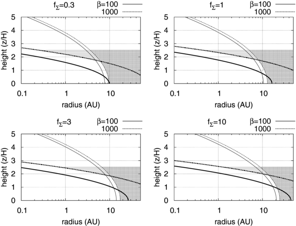
Figure 7. Unstable regions in the protoplanetary disks. The thin solid and thin dashed curves represent  for the cases where magnetic field strength β = 100 and 1000, respectively, inside of which is a dead zone if the MRI self-sustainment is not taken into account (SMUN00). The regions above the thick solid and thick dashed curves satisfy Equation (20) for β = 100 and 1000, respectively, and are sustained zones according to the work-heat balance model. We compare the unstable region predicted by SMUN00 to that predicted by our model for β = 1000. The unstable regions according to SMUN00's and our model are marked by vertical and horizontal stripes, respectively.
Download figure:
Standard image High-resolution imageFigure 8 shows the active and sustained zones for dust-to-gas ratio fd = 1, fd = 0.1, fd = 0.01 (the fiducial model), and fd = 10−4. The work-heat balance condition Equation (20) is not affected by changing the dust properties such as the dust-to-gas ratio fd or dust size ad. One can understand this by rewriting the condition Equation (22) in the following form:
This form does not include a term affected by the dust properties, such as the magnetic diffusivity. On the other hand, E'crit is inversely proportional to the electron mean free path lmfp, and is proportional to the gas number density.
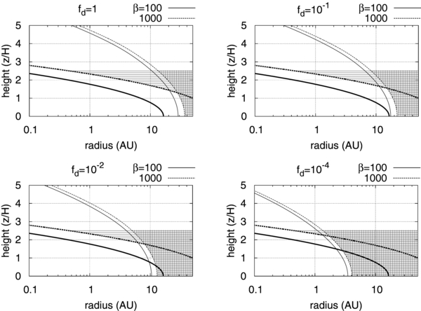
Figure 8. Unstable regions for different dust-to-gas ratios. The MRI unstable region according to (SMUN00) and our model are marked by vertical and horizontal stripes, respectively, for β = 1000.
Download figure:
Standard image High-resolution imageIn Figure 9, we study the evolution of the active and sustained zones as the gas density becomes lower while the dust density is kept constant. We change the set  from (1, 0.01) (the fiducial model) to (0.1, 0.1), (0.01, 1), and (10−4, 100). In Figure 9, zones are marked for β = 1000. The midplane of the disk between the radii 2 AU–20 AU becomes the sustained zone as the gas density becomes 10−4 times the fiducial model.

Figure 9. Change of unstable regions as the gas density of the disk decreases, while the dust density is kept constant. The MRI unstable region according to (SMUN00) and our model are marked by vertical and horizontal stripes, respectively, for β = 1000.
Download figure:
Standard image High-resolution image
4. CONCLUSIONS AND DISCUSSIONS
By performing numerical simulations of MHD with nonlinear Ohm's law of the three-dimensional local disks, we found hysteresis behavior for all the diffusivity models that we have tested: If we start from the laminar-flow initial conditions with small seed fluctuations, the MRI does not activate because of the diffusivity and the flow remains laminar; on the other hand, if we take an MRI turbulent state from an ideal MHD simulation as initial conditions, MRI remains active under the same diffusivity model. We surveyed three-parameter space (β, Jcrit, RM) in search of regions where the self-sustained MRI in the context of IS05 takes place. We found the condition, the work-heat balance model, for this hysteresis behavior to take place. The model is WJ ≲ Wsh, where WJ is the magnetic energy dissipated by Joule heating per unit volume and Wsh is the work done by background shearing motion per unit volume. This leads to the proportionality relation (Jcrit/Jeqp)(1/RM) ⩽ fwhb.
IS05 concluded that the energy supply from the shearing motion should be ∼30 times greater than the energy needed to supply enough ionization for the MRI, and it predicted the entire disk to be active. However, applying the work-heat balance model to various protoplanetary disk models, we have found that in most of the models, the sustained zone is above z/H > 2–3.
We conclude that in the fiducial protoplanetary disks environment the Joule heating (which has been neglected in IS05) becomes the dominant energy dissipation channel and constrains the self-sustainment of MRI, while the midplane of the disk remains dead. However, the gas of the disk dissipates (Alexander et al. 2006a, 2006b; Suzuki et al. 2010) within an observed timescale of 106–107 years (Cieza et al. 2007; Hernã¡ndez et al. 2008), while planetesimals remain and continue planet formation processes. In such a late phase of the disk, the sustained zone occupies a larger volume of the disk.
Although our nonlinear Ohm's law model is inspired by lightning phenomena, whether or not the Joule heating in this model takes the form of a spatially and temporally concentrated stream of ionizing electrons—lightning—has yet to be studied in future works employing nonthermal plasma studies. We limit ourselves to pointing out a few distinguishing properties of such lightning that make it an interesting subject. First, the work-heat balance model suggests that in sustained zones the major portion of shearing motion energy is converted to lightning. This means that lightning is one of the most dominant energy channels in the sustained zones. It will also pose a significant back-reaction to the accretion dynamics. We will need to reconsider the contribution of lightning in situations in which it has been neglected due to lack of energy, such as in chondrule formation (Weidenschilling 1997).
The second point is related to the redox environment that the lightning creates. Lightning induced by collisional charging of water ice dust overcomes the energetics problem (Muranushi 2010), but if applied as the chondrule heating source, it suffers from redox environment mismatch. Water vapor creates oxidizing environments (Clayton et al. 1981; Rubin 2005), whereas major populations of chondrules are considered to have formed in reducing environments (Lofgren 1989; Connolly et al. 1994; Jones & Danielson 1997). However, the lightning in sustained zones proposed by IS05 and studied in this paper is a result of a pure MHD process, and thus is redox-neutral. Therefore, it can potentially explain chondrule heating in both reducing and oxidizing environments.
T.M. thanks Yuichiro Sekiguchi and Masaru Shibata for useful discussions. We thank the referee for valuable comments. The simulations for this paper have been performed on the computer cluster at Kyoto University built by T.M. and on the TSUBAME2.0 Grid Cluster at Tokyo Institute of Technology. The use of TSUBAME2.0 in this project was supported by JHPCN through its program "Joint Usage/Research Center for Interdisciplinary Large-scale Information Infrastructures." This work is supported by Grants-in-Aid from the Ministry of Education, Culture, Sports, Science, and Technology (MEXT) of Japan, Nos. 24103506 (T.M.), 22.7006 (S.O.), 18540238, 23244027, and 23103005 (S.I.).