


ABSTRACT
The vertical structure of a post-impact, pre-lunar disk is examined. We adopt the equations introduced by Thompson & Stevenson for a silicate disk in two-phase equilibrium (vapor plus liquid) and derive an analytical solution to the system. This largely reproduces their low-gas mass fraction, x ≪ 1, profiles of the disk but is also employed to examine higher x cases. The latter are generally gravitationally stable and are used to develop a stratified disk model consisting of a gravitationally unstable magma layer surrounded by a stable, primarily vapor atmosphere. Initially, the atmosphere contains the majority of the disk mass, while the surface density of the magma layer is determined by requiring its viscous energy dissipation supply the disk's radiation budget. The magma layer viscously spreads on a ∼50 yr timescale during which vapor continuously condenses into droplets that settle to the layer, maintaining its surface density and dissipation rate. Material flowing outward, past the Roche boundary, can become incorporated into accreting moonlets, and this supply persists until the vapor reservoir is depleted in ∼250 yr.
Export citation and abstract BibTeX RIS
1. INTRODUCTION
The leading theory of lunar origin is via giant impact, in which a late-arriving Mars-sized impactor collides with the Earth during its final stage of accretion. The body makes an oblique collision that launches material from both objects into orbit around the Earth, and the Moon subsequently forms from this post-impact disk of debris. The concept of generating a lunar precursor disk by large impacts was proposed by both Hartmann & Davis (1975) and Cameron & Ward (1976), but it was the latter work that argued a Mars-sized object was required to satisfy angular momentum constraints of the Earth–Moon system. It is this scenario that has generally become regarded as the Giant Impact Hypothesis.
The collision event itself has been modeled extensively by smooth particle hydrodynamics (SPH) techniques, initially by Benz et al. (1986, 1987), Cameron & Benz (1991) and subsequently at higher resolution by Canup & Asphaug (2001) and Canup (2004, 2008). Figure 1 shows a representative simulation that generated a disk of sufficient mass to produce a lunar-sized satellite (Canup 2011). These simulations find that torques exerted by the deformed target were instrumental in modifying the debris trajectories following their launch to prevent their re-intersection with the Earth. The disk material was typically composed of 60%–80% from the projectile and 40%–20% from the target and is hot enough that a significant fraction of the material is vaporized.

Figure 1. Example SPH simulation of a giant impact that generates a disk of sufficient mass to produce the Moon. The material is color coded by temperature. The first panel is about 1.5 hr into the impact when the distortions of target and impactor are pronounced; the second panel is at about 30 hr post-impact where the material surrounding the Earth is settling into a hot vapor + liquid silicate disk. (Figure provided by R. M. Canup 2011.)
Download figure:
Standard image High-resolution imageFollowing its emplacement, the disk material interior to the Roche distance, aR ∼ 3 R⊕ (where R⊕ = 6.38 × 108 cm is Earth's radius), cannot undergo accretion due to tidal shear but will viscously spread, with some material being re-accreted by the Earth while the rest diffuses outward. Material flowing across the Roche boundary can be incorporated into accreting moon(s), which eventually coalesce into the Moon itself. The spreading timescale, τν ∼ a2R/ν, depends inversely on the strength of the disk viscosity, ν. The surface density of the disk is high; ∼1.5 lunar masses distributed over an area ∼π(a2R − R⊕2) implies an average density of σ ∼ 107 g cm−2. Ward & Cameron (1978) pointed out that the disk could become susceptible to gravitational instability if the dispersion velocity of its constituent components damped below a critical value (e.g., Goldreich & Ward 1973)

where Ω = (GM⊕/a3)1/2 is the orbital frequency of the disk material with M⊕ = 5.97 × 1027 g being the mass of the Earth. Evaluating Equation (1) at the disk mid-point, ∼2 R⊕ where Ω = 4.39 × 10⁻⁴ s−1 gives ccrit = 4.79 × 103 cm s−1. Since tidal stresses shear out the unstable clumps as they try to form, the overall result is to generate an effective viscosity of order

Using this in τν yields a short spreading time estimate of order ∼2 yr. As material crosses the Roche boundary, it can begin to quickly accrete into a moon. This rapid formation has been numerically simulated by, e.g., Ida et al. (1997) and Kokubo et al. (2000).
This timescale estimate was brought into serious question in an important (but perhaps under-appreciated) paper by Thompson & Stevenson (1988; hereafter TS88) who pointed out that so much dissipation occurs over such a short timescale, that it is likely the entire disk would vaporize and become gravitationally stable, implying a contradiction. The dissipation rate per unit area in a viscous Keplerian disk is of order

where Equation (2) has been used in the final form. This would heat the disk until it was hot enough to radiate away the energy at the rate

where σSB = 5.67 × 10⁻⁵ erg cm−2 s−1 K−4 is the Stefan–Boltzmann constant, Tph is the photospheric temperature, and the lead factor of two counts both sides of the disk. Equating Equations (3) and (4) implies a photospheric temperature of Tph ≈ 6700 K, far too high for condensed silicates. TS88 argue that a much lower photospheric temperature (Tph ∼ 2000 K) is more consistent with a disk where vapor and condensed phases co-exist and that this should ultimately limit the allowed rate of spreading. To be self-consistent, the effective viscosity would have to be much lower than Equation (2), i.e., νeff ∼ (2000/6700)4ν = 8.0 × 10⁻³ν. This, in turn, would imply a radiation-limited spreading timescale of order τrad ∼ 250yr.
To reconcile these two timescales, TS88 argued that the disk self-regulates itself by hovering on the brink of gravitational instability, i.e., a so-called metastable state. Since the sound speed of a single-phase silicate vapor gas disk would be of order c ∼ (γRT/μ)1/2 ∼ 7.4γ1/2 × 104(T/2000 K)1/2 cm s−1, where γ is the adiabatic index and μ ∼ 30 g mol−1 is used for the effective molecular weight of the vaporized rock (TS88), this is too high for instability. However, TS88 point out that a two-phase disk, in which vapor and condensed phases co-exist, can exhibit a much lower sound speed because of an increased compressibility of the system and could, in fact, be unstable under certain conditions.
2. DISK VERTICAL STRUCTURE
2.1. A Single-phase, Isothermal Reference Solution
A useful basis of comparison is the vertical structure of a hypothetical isothermal, single-phase silicate gas disk with a surface density σ = 107 g cm−2. The equations that govern the structure are the ideal gas equation

where P(z) is the pressure, T is the temperature, ρ(z) is the gas density, and R = 8.31 × 10⁷ erg mol−1 K−1 is the universal gas constant, and the equation of hydrostatic equilibrium,

where z is the vertical distance above the disk mid-plane. For a constant temperature T = T* = 2000 K, the sound speed-like quantity c* = (RT*/μ)1/2 = 7.44 × 104 cm s−1. Substituting Equation (5) into (6) and integrating leads to

where ρ* is the mid-plane density and

is the scale height.
Integrating ρ vertically yields the surface density, i.e.,
Substituting Equation (7) for ρ yields  , implying ρ* = 2.35 × 10⁻² g cm−3. Combining Equations (5) and (7) then gives

and a mid-plane pressure of P* = 1.3 × 10⁸ dynes.
Applicability of this type of structure to the lunar disk would depend on two implicit assumptions: (1) an opacity so low as to preclude any significant temperature gradient and (2) a disk too hot for the stability of a condensed phase. Neither of these conditions is likely to have prevailed in the post-impact silicate disk.
When the disk has a finite opacity, the temperature is no longer constant and decreases with height above the mid-plane z = 0. If the opacity is high enough, the temperature profile needed to satisfy the luminosity equation would be super-adiabatic. In this case, it is likely that the vertical heat flux is carried by convective transport and that the adiabatic equation

applies as well, where again  is the sound speed. Combining with Equations (5) and (6) leads to the well-known adiabatic profiles where P∝ργ. However, as stressed by Thompson & Stevenson (1988), if the both gas and condensed phase co-exist, there are additional constitutive equations to consider.
2.2. Constitutive Equations for Two-phase Disks
When two phases are present, there is a new state variable, x, representing the gas mass fraction; the condensed phase mass fraction then being 1 − x. One must now also distinguish between the gas density ρg and the total density ρ of the gas plus condensed phase mixture given by

where ρs denotes the density of the condensed phase. The total density must appear in the hydrostatic (Equation (6)) and adiabatic (Equation (11)) equations, but not in the ideal gas law (Equation (5)), where only the gas density ρg is to be used. In addition, when both phases are present, the temperature and pressure must satisfy the Clausius–Clapeyron phase equilibrium equation. TS88 approximate this by the relationship

with Po = 3 × 10¹⁴ dynes and To = μℓ/R = 6 × 10⁴ K, where ℓ = 1.7 × 10¹¹ erg g−1 is the latent heat of vaporization of silicates. These are the data primarily employed by TS88 and are due to Krieger (1967). We shall use them here as well to facilitate comparisons. We should caution that Equation (13) is an approximation because "silicates" do not volatilize congruently, e.g., SiO is a major gas phase, but there is no SiO solid.
Equation (13) gives the pressure as a function of temperature alone. Combining Equations (5) and (13) also allows the determination of the gas density as a function of temperature alone,
Finally, the sound speed appearing in Equation (11) must now be replaced by the two-phase sound speed (e.g., Landau & Lifshitz 1959; TS88) when both species can be present
where Cg = (3/2)RT = 4.16 × 10⁶ erg g−1 K−1, Cs ∼ 107 erg g−1 K−1 are the specific heats of the vapor and condensed phases. Using Equation (14) to eliminate ρg results in an expression for the sound speed that depends only on x and T. The two-phase sound speed is generally less than that of a single phase because the ability of gas to condense makes it more compressible. Figure 2 shows the behavior of the sound speed as a function of the gas mass fraction x for some representative temperatures.
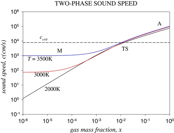
Figure 2. Two-phase sound speed as a function of gas mass fraction for various temperatures. The sound speed drops as the gas fraction decreases, but eventually levels off as the density approaches that of a pure liquid phase. The critical sound for the onset of gravitational instability at r = 2 R⊕ in a disk of surface density σ = 107 g cm−2 is shown for comparison. The sound speed becomes comparable to this when the gas mass fraction is of order x = 10−2.
Download figure:
Standard image High-resolution imageEquations (5), (6), (11), (12), (13), and (15) close the system, and the hydrostatic and adiabatic equations can be reduced to two equations for dT/dz and dx/dz, namely,
The details of this derivation are given in Appendix A. Generally, ρg ≪ ρs and the first factor in Equation (17) can be set to unity. For the cases of interest here, it is also likely that x/ρg ≫ (1 − x)/ρs in Equation (12), i.e., that gas occupies most of the volume even if the gas mass fraction is low (TS88). In that case, ρ/ρg ≈ 1/x and the equations simplify to
2.3. An Analytic Solution
To obtain a system solution we begin by dividing Equation (17') by (16') to find
where ΔC ≡ Cs − Cg. This can be integrated from the mid-plane values to give
where  denotes the exponential integral (e.g., Abramowitz & Stegun 1966). Equation (19) tells us for a given set of mid-plane values {xc, Tc}, how the gas mass fraction varies as a function of temperature, x(T). We already know P(T) and ρg(T) from Equations (13) and (14), respectively, but Equation (19) can now be used to find ρ(T) = ρg/x and c(T, x(T)). All that remains is to determine the height z(T) at which a given temperature is reached. To do this, we substitute Equation (19) into Equation (16'), and integrate leading to
where the integration limits are y ≡ ΔCT/ℓ, yc ≡ ΔCTc/ℓ. Integration by parts gives
and combining with Equation (20) yields
which completes the solution.
We note that for the values adopted here, ΔCT/ℓ = (Cs − Cg)T/ℓ = 0.0687(T/2000 K) is significantly smaller than unity and suggests that we can expand Equations (19) and (22) in that quantity. Setting ey ≈ 1 + y + ⋅⋅⋅, E1(y) ≈ −γ − ln y + y + ⋅⋅⋅, where γ = 0.5772 is Euler's constant, and keeping terms up to order y, Equation (22) reduces to
In writing the right-hand side, a new length scale, Ho ≡ (2ℓ)1/2/Ω =(2RTo/μ)1/2/Ω has been introduced. For the parameter values adopted here, Ho = 1.33 × 109 cm = 2.08 R⊕. Note that to this level of accuracy, ΔC does not appear. To get comparable accuracy in expanding Equation (19) we need only keep terms up to ln y because there is no factor of (ΔC)−1 in the coefficients. This results in
An alternative form for x can be found by using Equation (23) to eliminate the log term in Equation (24), i.e.,
Since the temperature decreases with height, the second term in Equation (25) increases the gas mass fraction while the last term decreases it. Which dominates depends on how high one must go for the temperature to drop to the photospheric value, Tph ∼ 2000 K.
Figures 3–5 show example disk profiles constructed from Equations (13), (14), (23), and (24) and ρ ≈ ρg/x. For the sound speed, the level of approximations used to derive Equations (24) and (25) suggests that we set ΔC → 0 and ignore the second term in the numerator of Equation (15) for consistency. The sound speed expression then reduces to
The adopted gas mass fraction at the mid-plane, xc, is progressive larger from Figures 3–5. However, for a given surface density, the choice of {xc, Tc} is constrained through Equation (9).
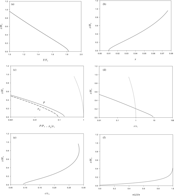
Figure 3. Vertical profile of a disk with mid-plane gas fraction and temperature values xc = 0.01, Tc = 3644 K. The panels depict the altitude z normalized to a reference length H* = 2.40 × 108 cm = 0.376 R⊕ vs. (a) the temperature T normalized to a reference value T* = 2000 K, (b) the gas mass fraction, (c) the pressure (solid line) and gas density (dashed line) normalized to reference values P* = 1.3 × 10⁸ dynes and ρ* = 2.35 × 10⁻² g cm−3, (d) the total density normalized to ρ*, (e) the sound speed normalized to c* = 7.44 × 104 cm s−1, and (f) the cumulative surface density normalized to its total value. The dotted lines in (c) and (d) show profiles for the isothermal reference solution from comparison.
Download figure:
Standard image High-resolution image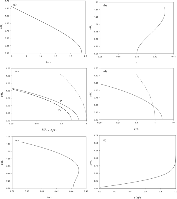
Figure 4. Same profile displays as Figure 3 except that the adopted mid-plane values for the gas mass fraction and temperature are xc = 0.1, Tc = 3898 K.
Download figure:
Standard image High-resolution image
Figure 5. Same profile displays as Figure 3 except that the adopted mid-plane values for the gas mass fraction and temperature arexc = 1, Tc = 4218 K.
Download figure:
Standard image High-resolution image2.4. Surface Density
The surface density in Equation (9) involves an integration over the altitude, z. However, in our solution for the profile, the temperature has been employed as the independent variable. One can switch to an integration over T as follows:
In the first step, we stop the integration at the photospheric height zph = z(2000 K) with little error since the density has become very low and there is little mass beyond that point. The second step switches to T as the integration variable, while step three replaces ρ = ρg/x and uses Equation (16') to remove the derivative. Interestingly, the gas mass fraction cancels out at this point. In the final two steps, Equations (1) and (13) to used to eliminate ρg and P, respectively. In the integration, Equation (23) is to be used for z(T) which contains the mid-plane gas mass fraction, xc, as part of the expression so that ultimately σ = σ(xc, Tc). Requiring σ(xc, Tc) = 107 g cm−2 then constrains the allowable combinations as shown in Figure 6. In particular, assumed values of xc =(0.01, 0.1, 1) require mid-plane temperatures of Tc = (3644 K, 3898 K, 4218 K) respectively, and these were used in the construction of the disk profiles.
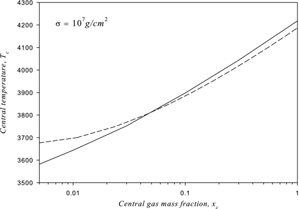
Figure 6. Mid-plane temperature Tc required as a function of the mid-plane gas mass fraction xc to ensure the surface density of the disk is σ = 107 g cm−2. The solid line is obtained by a numerical integration of the profile equations over T; the dashed line is an approximate analytical relationship found by integrating the density over z by the method of steepest descent.
Download figure:
Standard image High-resolution image
2.5. Approximate Solutions for Small Temperature changes
Although the roughly factor of two change in temperature from the mid-plane to the photosphere occurs over an altitude zph comparable to or greater than H*, the e-folding distance for the pressure (and density) is much less, especially at low values of xc. This is due in part to phase equilibrium as mandated by the Clausius–Claperyon equation. The pressure at mid-plane is  , while the temperature, Te, at which the pressure drops by a factor e−1 is given by −To/Te = −To/Tc − 1, implying a temperature change of
  which is typically of order ∼0.06. This suggests that we can set
  where
where  and Taylor expand Equation (23) to find
which, solving for T, gives
Using this in Equation (25) then implies
In practice, however, the second term in the bracket of Equation (28) is of order O(10−2) for  so that keeping only the leading linear term is reasonably good unless xcis very small. In this case, we can write Equations (28) and (29) to lowest order as
From these it is easy to see that while the temperature decreases with height, whether the gas mass fraction decreases or increases from the mid-plane depends on whether xc is greater or less than CsTc/ℓ.
We return now to the Clausius–Clapeyron equation and write
where another new length scale Hc ≡ (2RTc/μ)1/2/Ω is introduced. The pressure scale height is of order  so that decreasing the gas mass fraction thins the disk vertically as is evident in the disk profiles of Figures 3–5. Since (Hc/Ho)2 = Tc/To, x−1c(z/Ho)2 can still be small when (z/Hp)2 ∼ O(1). An estimate of the density is now obtained from ρ = μP/xRT, namely,
Equation (33) can be used to derive an approximate analytic expression for the surface density  This integral can be estimated by the method of steepest descent (Appendix B),
which can be rearranged to give xc = xc(σ, Tc),
This is compared with the numerical integration in Figure 6. The agreement is reasonably good but becomes less accurate at low x-values where the linear expressions of Equation (31) are less suitable.
3. CONTINUOUS DISK MODELS
3.1. Low Gas Mass Fraction Models, x ≪ 1
Figure 3 illustrates a disk with x = 0.01 and mid-plane temperature Tc = 3644 K. Figure 3(a) shows the temperature (abscissa) normalized to T* = 2000 K versus height (ordinate) normalized to the scale height, H* of the isothermal reference solution. The temperature decreases with z at a nearly constant rate. Figure 3(b) displays the gas mass fraction that increases steadily with height until reaching between 7% and 8% at the photosphere. In contrast, the pressure and gas density in Figure 3(c) decreases much more precipitously, as does the full density in Figure 3(d). However, whereas the gas density at the mid-plane is smaller than that of the isothermal model, the total density is larger. This latter reflects the fact that the effective scale height is much less than H* as discussed in the last section. For comparison, the density for the isothermal disk is included as a dotted line in the graphs. Figure 3(e) plots the sound speed behavior (normalized to c*) with height. The sound speed increases through most of the disk, but hits a maximum near z/H* ∼ 0.8. Figure 3(f) displays the cumulative surface density with altitude. The bulk of the surface density resides within ∼0.1H*, consistent with the total density profile.
Thompson & Stevenson (1988) concentrate on models with low gas fractions x ⩽ O(10−2), which they liken to a foam. Their strategy is to adopt a gas fraction low enough to trigger marginal gravitational instability. This is schematically represented by the TS-label in Figure 2. The mid-plane sound speed when 1 − x ∼ O(1) reads  . This is below the critical sound speed equation (1) for xc ⩽ 5.3 × 10⁻³. For this value, the temperature is Tc = 3588 K and the central pressure and gas density are
  and ρg, c = μPc/RTc = 1.61 × 10⁻³ g cm−3, respectively. The length scale Hc = 3.22 × 108 cm, but the pressure scale height is only
  . In this case, the corresponding central total density is ρc = ρg, c/xc = 0.303 g cm−3. Comparing central quantities to the isothermal reference model, Tc/T* = 1.79, Pc/P* = 0.126, ρg/ρ* = 0.0685, ρc/ρ* = 12.9, and Hp/H* = 0.098. As in Figure 3, the gas density is less, but the total density is over an order of magnitude greater than the reference profile. Again, the preponderance of the mass is in the liquid phase.
3.2. Tuning the Dissipation through ν
To understand how TS88 propose a metastable state can lower the effective viscosity, consider the dispersion relationship for horizontal oscillations of a self-gravitating, Keplerian disk (e.g., Goldreich & Ward 1973),

where ω is the oscillation frequency and k is the wave number of the mode. The minimum of this expression is where dω2/dk = 0 for which kmin = πGσ/c2 and ω2(kmin ) = Ω2[1 − (πGσ/cΩ)2]. Marginal stability occurs when ω2(kmin ) = 0, i.e., at ccrit → πGσ/Ω and kcrit = Ω2/πGσ. For c < ccrit, ω2 = −Ω2[(ccrit/c)2 − 1] and ω = ±iΩ[(ccrit/c)2 − 1]1/2 becomes imaginary, implying a growing mode on a timescale τinst = Ω−1[(ccrit/c)2 − 1]−1/2. This is longer than the timescale ∼O(Ω−1), to shear out clumps, suggesting that the perturbation velocities, vinst, generated by the instability achieve a value less than ccrit by a factor ∼1/Ωτinst. This implies a viscosity, νeff ∼ (vinst)2/Ω, less than the nominal value of Equation (2) by a factor 1/(Ωτinst)2 = (ccrit/c)2 − 1. Setting this equal to 8.0 × 10⁻³ results in a viscous spreading timescale comparable to the radiation timescale and implies c = 0.996ccrit.
This is an elegant concept, but one caveat of the model is that the liquid and vapor phases must be well mixed throughout the structure. Thompson & Stevenson (1988) caution that this may not be satisfied and that some settling could occur. This could lead to another class of models that are stratified with a highly unstable magma layer surrounded by a stable vapor reservoir. We turn to such a possibility in the next section.
4. STRATIFIED DISK MODELS
The possibility of a stratified pre-lunar disk has been considered by Machida & Abe (2004). They concluded that a particle layer would form quickly by settling and then spread on the timescale comparable to that estimated in earlier particle models (i.e., Ward & Cameron 1978; Ida et al. 1997; Kokubo et al. 2000). Their paper contains several insightful features including droplet settling and growth timescales, a model of boundary layer turbulence using the formulism of Sekiya (1998), and a more accurate version of gravitational instability for an incompressible fluid disk due to Sekiya (1983). However, their treatment is actually similar to a two-phase two-component disk because the phase equilibrium physics was not included. Thus, there was no limitation on the amount of material that could collect in the magma layer. In this section, we will describe a stratified model including phase physics that assumes a relatively high x atmosphere over an unstable magma layer whose surface density is regulated by the radiation budget.
4.1. Moderate to High Gas Mass Fraction Models, x ⩽ 1
Figure 4 presents the disk profile for xc = 0.1, Tc = 3898 K. The temperature again deceases with height at a fairly constant rate, but the photosphere is higher. Interestingly, the gas mass fraction at first increases, but reaches a maximum of ∼13% near z/H* ∼ 1.35. Pressure and densities still drop quickly, but with an e-folding distance about three times that of Figure 3 consistent with the ∼ dependence of the effective scale height. As a result of the increased disk thickness, the gas density and total density, although still less than and greater than ρ* respectively, are closer to that value. In Figure 4(d), we see that the sound speed is no longer monolithic with height. Although it increases during most of the cumulative surface density (shown in Figure 4(f)), it decreases in the higher altitude, more rarefied portion of the structure.
In Figure 5, the mid-plane gas mass fraction is assumed to be unity and the temperature Tc = 4218 K. For high x the sound speed is approximately
The mid-plane sound speed is cc = 1.09 × 10⁵cms−1, which is far too high for gravitational instability. However, now both the gas mass fraction (Figure 5(b)) and sound speed (Figure 5(e)) monotonically decrease with altitude. The scale height Hp ∼ Hc = 3.49 × 108 cm, which is over an order of magnitude greater than the low x disk considered in Section 3.1. The corresponding central pressure is Pc = 1.99 × 10⁸ dynes and the central gas density is ρg, c = 1.67 × 10⁻²gcm−3. Since xc = 1, this is also the total density ρc. Compared to the isothermal reference model, Tc/T* = 2.11, Pc/P* = 1.53, ρg, c/ρ* = ρc/ρ* = 0.427, Hp/H* = 1.45. These are not too different from the isothermal case, although the two-phase disk is a little thicker. Note that in this model, most of the mass resides in the vapor state.
4.2. Tuning the Dissipation Rate Through σ
If the disk is stable but continues to radiate, the energy losses are compensated by latent heat release through condensation. Assuming that the droplets can settle, a magma layer will begin to collect in the mid-plane. The magma layer can itself be susceptible to gravitational instability. This is not just because the sound speed is low if the gas mass fraction is very small in the layer, but also because a typical parcel of the magma can be large enough that it is not well coupled to the gas through drag forces. The layer is not metastable but undergoes vigorous dissipation with an effective viscosity given by the original Ward–Cameron expression, Equation (2). The dissipation obtained from Equation (3) is at first insufficient to satisfy radiation losses, but as the layer density builds up, the dissipation rate climbs. The critical surface density at which these rates are comparable is found be equating dE/dt = F to find

At a = 2 R⊕, Tph = 2000 K this reads σcrit ≈ 2 × 10⁶ g cm−2, which is about ∼1/5 of our assumed starting surface density value. The remaining ∼4/5 of the material resides in the stable atmosphere above the mid-plane. This configuration is represented schematically in Figure 2 by the labels A and M indicating the atmosphere and magma layer. Substituting Equation (38) into (2) and using this in the estimated spreading timescale yields, τν ∼ 50 yr. As material spreads across the Roche boundary and into the Earth at the inner boundary, the surface density of the magma layer goes down and so does its energy dissipation. As it drops below the radiation rate, more material condenses and settles to replenish the magma layer. This cycle continues until the vapor atmosphere is exhausted in ∼250 yr. This constitutes an alternative way in which viscous and radiation time scales can be reconciled.
4.3. Boundary Layer Drag
An additional complication arises for a stratified disk where there is an interface between the magma layer and atmosphere. This can introduce boundary layer drag that can decay the orbits of the magma layer on a timescale as short as a few years. This is due to loss of angular momentum to the vapor atmosphere which can be sub-Keplerian if an outward pressure gradient partially supports it. This issue was also considered in the treatment of Machida & Abe (2004) assuming a constant ratio of the radial pressure force to Earth's gravity. However, since there is no external torque, the entire disk cannot destroy itself. Material lost to the Earth has a lower specific angular momentum than the rest of the disk so that the specific angular momentum of the latter must increase. To accommodate this, the disk restructures itself with an outward migration of vapor that tries to remove the pressure gradient and shut off the boundary layer drag. To illustrate, consider a power-law disk, σ∝r−n, of mass Mn that extends from r = R⊕ to 3R⊕. The disk angular momentum is  Mnj⊕(2 − n)(35/2 − n − 1)/(5/2 − 1)(32 − n − 1), where j⊕ ≡ (GM⊕R⊕)1/2 denotes the specific angular momentum if orbiting at Earth's radius. Suppose the initial disk has a 1/r dependence for which L1 = 1.40M1j⊕. If the disk restructures itself to a constant surface density, its angular momentum will be L0 = 1.46M0j⊕. During the process, the Earth absorbs an angular momentum ΔL = (M1 − M0)j⊕ carried by the disk material that decays into it. Conservation of angular momentum requires that ΔL = L1 − L0 from which we conclude that M0 = 0.87M1, indicting that ∼13% of the disk is sacrificed to flatten the density gradient.
5. CONCLUSION
Assuming the Moon formed from an impact-generated disk, the manner and timing by which material spreads out from the Roche interior portion of the disk is an important boundary condition to determining the accretion history of the Moon. Early estimates of this spreading timescale were very short, ∼O(1) year, and depended on an effective viscosity generated by gravitational instability in the disk. On the other hand, the amount of energy viscously dissipated is enough to vaporize the disk, rendering it gravitationally stable unless there is time for the energy to be radiated away. Silicate vapor and liquid phases can co-exist when the photospheric temperature is of order 2000 K. If the phases are well mixed throughout the disk, the radiation rate of the disk at that temperature can limit the rate of spreading to a timescale of ∼O(102) yr. The implied lower viscosity could result from the disk hovering on the brink of instability with a sound speed just barely below the critical value for growing oscillation modes (Thompson & Stevenson 1988). A sufficiently low sound speed could characterize a two-phase disk, but requires a very low gas mass fraction of only a few percent. Keeping the condensed phase material suspended in so little gas seems problematic.
Here, we have pursued an alternative structure in which liquid droplets settle to the mid-plane and create a magma layer. This layer is subject to vigorous gravitational instability as originally suggested by Ward & Cameron (1978), but it does not contain the total surface density. The surface density is instead regulated by the phase equilibrium to be just that needed to supply the radiation budget through viscous dissipation, i.e., σ ∼ 2 × 10⁶ g cm−2, which is of order 20% of the average starting value assuming 1.5 lunar masses are initially in the Roche interior portion of the disk. The bulk of the material resides in a stable atmosphere. As the magma layer spreads viscously on a ∼50 year timescale, its surface density and viscosity would tend to decrease, causing the dissipation rate to become insufficient to compensate for radiation losses from the disk photosphere. These losses are made up by condensation in the atmosphere which releases latent heat. The condensed droplets settle to the magma layer restoring its surface density to the critical value. This cycle continues until the vapor reservoir is exhausted, which takes a total of ∼250 yr.
The total timescale is quite similar to that predicted by Thompson & Stevenson (1988) because it is still regulated by the radiation rate. However, the manner in which material is fed to a forming Moon is significantly different. TS88 proposed that, being in a metastable state, the disk could spread beyond the Roche boundary without immediately fragmenting. Thus, the entire disk spreads as a unit during which its increased areal extent results in a decreased surface density. Fragmentation would occur when the surface density dropped to the point that full-scale instability was needed to supply the radiation budget through viscous dissipation. A similar criterion is used in our stratified model except that the critical surface density is achieved by limited condensation. Thus spreading of material beyond the Roche boundary occurs earlier and accretion of the material into moons can commence closer to aR. The radiation timescale now sets the interval over which material is continuously supplied to the accretion zone, an important boundary condition for lunar accretion models. Detailed models of the disk's radial evolution and lunar accretion will be addressed in upcoming works.
This work was supported by grants from NASA's LASER program and by the NASA Lunar Science Institute (NLSI).
APPENDIX A
Differentiating Equation (13) we find that
Combining with the ideal gas law then gives
and using this in the hydrostatic Equation (6) results in Equation (16) in the main text. To obtain dx/dz, we first use Equation (6) to eliminate dP/dz in Equation (11), i.e.,
Next, use the fact that ρ−1dρ/dz = −ρd(1/ρ)/dz to write
Taking the derivative and rearranging,
From the ideal gas law, Equations (A1) and (16), it follows that
and substituting this into Equation (A5) we find
Finally, the expression for c2 is used to reduce the final bracket to
by recalling that ℓ = RTo/μ and setting μ/RT = (To/T)/ℓ. This leads to Equation (17) in the text. In a preliminary treatment of the high x case (Ward 2011) only the leading term in the sound speed was used, i.e., Equation (22). This led to an error in the sign of dx/dz. This is because the leading term which produces the To/T term in the second bracket on the left-hand side of Equation (A8) is identically canceled by such a term in the first bracket. Thus, the secondary terms in 1/c2are pivotal to the derivative. Omitting them causes Equation (A8) to read +x/ℓ.
APPENDIX B
To integrate the density vertically to find the surface density we have used an approximation due to the method of steepest descent. The surface density is given by  . Substituting Equation (33)
where the parameter t ≡ z/Hp = (xc)−1/2(z/Hc) is introduced and a ≡ (CsTc/ℓxc − 1)Tc/To, b ≡ Tc/To. Next the integrand is written in the form exp [ − t2 − ln (1 + at2) − ln (1 − bt2)] = exp [ − f(t)]. The function f(t) is expanded in a Taylor series about its minimum where df/dt = 0. Since
the minimum is at t = 0 where f(0) = df/dt = 0 and f(t) ≈ (1/2)f''(0)t2 = (1 + a − b)t2. Consequently, the integral is approximately,
Substitution into Equation (B1) gives Equation (34) in the text.