


ABSTRACT
The ARCADE 2 instrument has measured the absolute temperature of the sky at frequencies 3, 8, 10, 30, and 90 GHz, using an open-aperture cryogenic instrument observing at balloon altitudes with no emissive windows between the beam-forming optics and the sky. An external blackbody calibrator provides an in situ reference. Systematic errors were greatly reduced by using differential radiometers and cooling all critical components to physical temperatures approximating the cosmic microwave background (CMB) temperature. A linear model is used to compare the output of each radiometer to a set of thermometers on the instrument. Small corrections are made for the residual emission from the flight train, balloon, atmosphere, and foreground Galactic emission. The ARCADE 2 data alone show an excess radio rise of 54 ± 6 mK at 3.3 GHz in addition to a CMB temperature of 2.731 ± 0.004 K. Combining the ARCADE 2 data with data from the literature shows an excess power-law spectrum of T = 24.1 ± 2.1 (K) (ν/ν0)−2.599 ± 0.036 from 22 MHz to 10 GHz (ν0 = 310 MHz) in addition to a CMB temperature of 2.725 ± 0.001 K.
Export citation and abstract BibTeX RIS
1. INTRODUCTION
The standard big bang model places the formation of the cosmic microwave background (CMB) at z ≈ 6 × 10⁶ with a nearly perfect blackbody spectrum. The blackbody spectrum remains in thermal equilibrium with the electrons and ions in the early universe until the surface of last scattering at z = 1089. Measurements by the Far Infrared Absolute Spectrophotometer (FIRAS) instrument across the peak of the CMB spectrum (∼60–∼600 GHz) limit deviations from a blackbody, with temperature 2.725 ± 0.001 K, to be less than 50 parts per million (Fixsen & Mather 2002; Fixsen et al. 1996), but measurements at centimeter or longer wavelengths are less restrictive. Plausible energy-releasing processes including star formation and particle decay or annihilation could produce observable distortions at centimeter or longer wavelengths while evading constraints at millimeter wavelengths.
At radio frequencies below 10 GHz, the radiation from the sky is increasingly dominated by synchrotron and free–free emission both from our own Galaxy and distant point sources and perhaps distant diffuse sources. The Absolute Radiometer for Cosmology, Astrophysics and Diffuse Emission (ARCADE 2) instrument observes the CMB spectrum at frequencies a decade below FIRAS to observe the spectrum at the highest frequency where there is a significant contribution from the radio background.
2. THE INSTRUMENT
ARCADE 2 is a balloon-borne double-nulled instrument with seven radiometers at frequencies of 3, 5, 8, 10, 30, 30, and 90 GHz mounted in a liquid helium bucket dewar. Each radiometer consists of cryogenic and room temperature components. A cryogenic Dicke switch operating at 75 Hz alternately connects the amplification chain to either a corrugated horn antenna (Singal et al. 2005) or an internal reference load (Wollack et al. 2007). The temperature of the reference load can be adjusted to produce zero differential signal, nulling the radiometer output. The horn in turn views either the sky or an external blackbody calibrator. The blackbody temperature can be adjusted to match the sky temperature, nulling instrumental offsets.
The external calibrator (Fixsen et al. 2006) has reflection of less than −45 dB and can be positioned to fully cover the aperture of any of the horns. Residual reflections from the calibrator are effectively trapped within the horn/calibrator system. Within this system, the calibrator absorbs almost all of the radiation because the horn emissivity is low and the calibrator emissivity is high. The effect of reflection from the calibrator system is proportional to the difference in temperature between the calibrator and the horn antenna throat.
To minimize instrumental systematic effects, the horns are cooled and maintained at a nearly constant temperature (∼1.5 K). The horns have a 12° full width at half-maximum beam and are pointed 30° from the zenith to minimize acceptance of balloon and flight train emission. A helium cooled flare reduces contamination from ground emission. No windows are used. The ambient atmosphere during flight is kept from the instrument by the efflux of helium gas.
After the switch, a GaAs high electron mobility transistor (HEMT) amplifier boosts the signal. The signal passes then through a thermal break to a 280 K section where it is further amplified and separated into two sub-bands followed by diode detectors, making 14 channels in all. Helium pumps and heaters allow thermal control of the cryogenic components which are kept at 2–3.5 K during the observations. The signal from each detector is demodulated with a lockin amplifier operating synchronously with the Dicke switch. The critical parameters of the radiometers and a full discussion of the instrument are given in Singal et al. (2011).
The sky temperature measurement depends critically on the calibrator temperature determination. The other components (horn, switch, cold reference, and amplifier) become a transfer standard while comparing the sky measurements to the calibrator measurements. There are 26 thermometers embedded in the calibrator, from the tips of the calibrator cones to the back of the calibrator, along with nine other thermometers on other parts of the calibrator to measure the temperature of its surroundings. These were included to look for gradients and other artifacts as well as to provide redundancy in the case of a thermometer failure. These ruthenium oxide thermometers (Fixsen et al. 2002) and the thermometers on the reference loads are read out at 0.9375 Hz with 2 mK precision and 1 mK accuracy (after averaging several samples). Identical thermometers have been calibrated on separate occasions over five years with absolute calibrations stable to less than 2 mK. Another 54 thermometers calibrated to ∼10 mK were distributed over other parts of the ARCADE 2 instrument.
3. THE OBSERVATIONS
The ARCADE 2 instrument was launched from Palestine, TX on a 29 MCF balloon in 2006 July 22 at 1:15 UT. The instrument reached a float altitude of 37 km at 4:41 UT. The cover protecting the cryogenic components was opened at 5:08 UT. The calibrator was moved 28 times from 5:30 to 8:11 providing at least eight cycles between calibrator and sky for each of the radiometers. During this time, the entire gondola with the instrument was rotated at ∼0.6 rpm, observing 8.4% of the full sky.
The 5 GHz switch failed in flight, so there are no useful data from that radiometer. One of the 30 GHz radiometers has a narrower beam which does not match the beams of the other radiometers and has much higher noise than the other 30 GHz radiometer so its data are not used here.
The most useful observations were from 5:35 to 7:40 UT and all of the following derivations will use various subsets of this data. During this time, the calibrator temperature was controlled between 2.2 and 3.1 K with a mean temperature of 2.72 K. A selection of 25 minutes of raw data from the flight (approximately 10% of the useful data) are shown in Figure 1. Only one of the channels for each radiometer is shown. The other channel is similar. Full scales on these plots are ∼1 K for the 3, 8, and 10 GHz radiometers, ∼3 K for the 30 GHz radiometer, and ∼2 K for the 90 GHz radiometer. While the 3 GHz radiometer observes the calibrator, the 8 GHz radiometer observes the sky, and the 10, 30, and 90 GHz radiometers "observe" the flat aluminum underside of the carousel. The 10, 30, and 90 GHz radiometers observe the sky or calibrator together. The Galactic crossings are clearly evident in the 3 GHz and 8 GHz sky data. Reference load changes can be seen in both the sky and calibrator in the 10 GHz and 90 GHz data. The 30 GHz radiometer data have much higher intrinsic noise. A first approximation to the sky temperature can be obtained by selecting an interesting sky datum on the figure and moving across to an appropriate calibration datum then reading off the calibrator temperature for that datum.

Figure 1. Subset of raw data from the flight. Full scales on these plots are ∼1 K for the 3, 8, and 10 GHz radiometers, ∼3 K for the 30 GHz radiometer, and ∼2 K for the 90 GHz radiometer. While the 3 GHz radiometer observes the calibrator, the 8 GHz radiometer observes the sky etc. The 10, 30, and 90 GHz radiometers view the sky or calibrator as a group. Intermediate transients have been suppressed. The Galactic crossings are clearly evident in the 3 GHz and 8 GHz sky data. Reference load changes can be seen in both the sky and calibrator in the 10 GHz and 90 GHz data.
Download figure:
Standard image High-resolution image4. SKY TEMPERATURE ESTIMATION
Conceptually, the calibration process is straightforward. The calibrator is placed over a radiometer horn, and the reference and calibrator are each warmed and cooled to allow the measurement of the emission coupling from each component into the radiometer. The radiometer output is modeled as a linear combination of component temperatures:

where T is a matrix of the relevant temperatures with each row a component and each column a time. The radiometer outputs are a vector, R. The solution, A, contains the couplings to the various parts of the radiometer. Since the lockin has both a positive and negative phase the couplings can be either positive or negative. The coupling parameters include the gain as well as the emissivity. The calibrator is then moved away so the radiometer observes the sky; the parameters measured while observing the calibrator can then be used to deduce the temperature of the sky. As the mathematics are developed, it is important to remember that the essential comparison is between the sky and the calibrator which brackets the sky temperature while the rest of the radiometer is in a similar state.
The most efficient use of the data uses all of the component temperature variations to obtain the best coupling estimates. However, some of the variations occur while the radiometer is observing the sky, which because of the beam scanning the sky includes the Galactic variation as well. The data could be binned by sky pixel and a solution made for each point, but that would not take advantage of the instrument variations happening while observing other pixels. Instead, a Galaxy model developed in a companion paper (Kogut et al. 2011) is subtracted at each pixel so only the uniform component remains. Then a general least-squares fit is used to solve for the emissivities, gain, and the uniform sky temperature simultaneously, including all of the sky observations.
The Galaxy model is derived iteratively. For the first iteration, the Galactic model is zero. The residual calibrated time series, combined with pointing data, is then used to generate a map as in Figure 1 of Kogut et al. (2011). The multi-frequency sky maps are combined to form a model of Galactic emission, which is then used to correct the time-ordered data for subsequent iterations of the sky solution. The Galaxy model depends on the spatial variation while the uniform sky temperature depends on the zero level so the convergence is very rapid. Since the model here implicitly assumes a uniform sky no variations are injected into the Galactic model from the fit. However, the uniform sky temperature depends on the absolute level of the Galactic model.
4.1. Galactic Foreground Subtraction
The Galactic foreground is complicated. A companion paper (Kogut et al. 2011) describes the detailed model produced using the ARCADE 2 data at 3, 8, and 10 GHz along with published results from sky surveys at higher and lower frequencies. The spatial structure of Galactic radio emission is modeled as a linear combination of template maps based on the 408 MHz survey (Haslam et al. 1981) and the full sky C ii map from Fixsen et al. (1999). The offset of the template model is then adjusted to match the total Galactic emission toward a set of reference lines of sight.
The distinction between Galactic and extragalactic radiation varies from author to author. We define the Galactic emission along selected lines of sight using two independent techniques. The first method treats the Galaxy as a plane-parallel structure, and bins the temperature of the ARCADE 2 sky maps and low-frequency radio surveys by the  to determine the Galactic emission at the north or south galactic poles. A second technique uses atomic line emission to trace Galactic structure. We correlate the ARCADE 2 or radio data against the map of C ii emission to determine the ratio of radio to line emission in the interstellar medium. We then multiply this ratio by the observed C ii intensity toward selected lines of sight (north or south galactic poles plus the coldest patch in the northern sky) to estimate the radio emission associated with the Galaxy along each line of sight. The two techniques agree well along each independent line of sight. The process is repeated at each frequency. The errors are necessarily correlated so a full covariance matrix is used to treat the uncertainty. The three lines of sight provide consistent estimates for the offset in the template model, with scatter 5 mK at 3 GHz and less than 1 mK at 8 or 10 GHz.
4.2. Calibrator Thermometry
Selecting which thermometer to use for the calibrator in the least-squares solution would be trivial if there were only one thermometer or all of the thermometers read the same temperature. Using many thermometers in the equation allows the radiometer data themselves to select the best linear combination to describe the radiometer data. However, the best differentiation of the various thermal modes of the calibrator is data from the times that the calibrator is moving or rapidly changing temperature. Unfortunately, these data cannot be used as they are taken during the calibrator movement or when the thermal state of the calibrator is poorly determined.
One way out of this dilemma is to make a thermal model of the calibrator using all of the data, then use that model during the times when the thermal and radiometric state of the calibrator is best understood to calibrate the radiometer. This has the advantage that the data can be used for the calibrator model even when the calibrator is being observed by a different radiometer.
A straightforward way of generating a model of the calibrator is to use principle component analysis (PCA) to extract the most essential calibrator modes. The calibrator has 24 thermometers embedded in the absorber to measure its temperature. A set of 21 of these thermometers was carefully recalibrated after the flight. The data from these thermometers are arranged as a matrix T of 21 rows of measurements each 6996 measurements long, corresponding to over 2 hr of observation. The eigenvector decomposition is

where D is a diagonal matrix of 21 eigenvalues and V is a set of 21 eigenvectors such that V · VT = I. This set of eigenvectors describes and organizes the data into modes. The corresponding eigenvalue calibrates the importance of each mode.
One of the critical differences between these modes is the response time of each mode. The best data to distinguish the time constants are the first few seconds after a thermal shock such as the movement of the carousel. The first eigenmodes exhibit the crucial thermal dynamics while the last eigenmodes are residual noise.
If the calibrator were perfectly isothermal the first (largest) eigenvalue would contain all of the variance and the corresponding eigenvector would equally weight each of the thermometers. In fact, the largest eigenvalue has 99.9% of the variance and the weights for the various thermometers only vary by ∼5% in the eigenvector.
The second largest eigenmode (0.08% of the temperature variance) is a front to back gradient in the calibrator. Such a gradient was anticipated based on heat flow from the 2.7 K calibrator to the colder (1.5 K) aperture below. A wrap-around tank of superfluid liquid helium surrounds the back and sides of the calibrator structure to intercept heat from the outside. A thermally conductive aluminum shield lies between the tank and the absorbing cones to provide an isothermal surface at approximately 2.7 K. The face of the calibrator opens to an aluminum plate maintained at the bath temperature (1.5 K). While the calibrator does not touch the plate, the diffuse (∼300 Pa) helium gas column can transport heat from the absorbing cones to the plate. The resulting heat flow creates a thermal gradient within the calibrator, which we measure using thermometers embedded within the absorbing cones.
Figure 2 compares the measured gradient to the locations of the thermometers within the cones. The total front to back gradient is approximately 600 mK; however, since most of the gradient occurs near the cone tips, 97% of the absorber volume remains within 10 mK of the base temperature. The thermometer locations were chosen using a simple static thermal model (Fixsen et al. 2006) and are concentrated near the cone tips. The thermometers are approximately uniformly distributed along the actual gradient so that in-flight gradients are well sampled throughout the absorber volume.
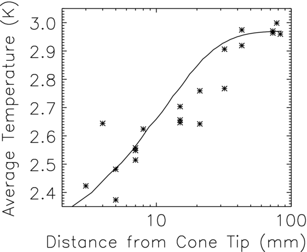
Figure 2. Temperature within the calibrator averaged over the data period vs. the distance from the tip (point). The line is the preflight prediction of the shape of the gradient. The preflight prediction was used to select the placement of the thermometers. It is not used in the analysis. The 21 thermometers are concentrated near the tips to fully sample the gradient. Some of the dispersion of the measured points is due to the radial gradient which is not shown here.
Download figure:
Standard image High-resolution imageThe details of the metal surface under the calibrator change as the calibrator moves from one position to another. We observe with the calibrator in one of three positions. While over the high-frequency horns, most of the calibrator is over a flat aluminum plate lying 1.5 mm below the cone tips. A few individual cones lie over the high-frequency horn antennas, with a larger gap between these cone tips and the aluminum wall of the horn. The 3 GHz horn is nearly the same size as the calibrator. While over the 3 GHz horn, most of the cone tips are ∼150 mm from the aluminum wall of the horn. The third position has roughly half the cone tips near the aluminum aperture plate and the other half suspended above the 5 and 8 GHz horns. The third and fourth eigenmodes show the imprint of the large change in thermal conductivity between the cones and the 1.5 K aperture corresponding to differences in the height of the gas column below each cone as a function of calibrator position. The thermal imprint of the three positions can be considered three vectors. Since the mean gradient has already been removed, there remain only two dimensions. The third and fourth eigenmodes span this space. Together the first four eigenmodes account for 99.98% of the temperature variance.
Smaller modes are more difficult to identify with known thermal conditions but may reflect changes in helium flow or changes in the aperture temperature during different times of the flight. We include the next six modes to be conservative. This accounts for 99.996% of the variation of the thermometers. The residual is roughly consistent with noise. Thus, we can describe the thermal state of the calibrator with

where V' is V truncated to 10 rows.
4.3. The Solution
A linear model can then be used to predict the radiometer output:

where g is the responsivity of the radiometer, X is the matrix of 10 thermal modes, U (each row is a mode, each column a time) augmented by rows for the sky temperature, the reference load temperature, the horn temperature, the switch temperature, and a fifth-order polynomial. E is a vector of emissivities and R is a vector of radiometer readings. Since the radiometer is followed by a lockin the sign of E is positive for the horn and calibrator but negative for the reference load. Some components (e.g., the switch or some of the gradients) can have either sign depending on the details of the unwanted asymmetries. Since neither g nor E is known a priori, they are combined; A = gE. A least-squares fit

produces the weighted solution to the optimum parameterization A, where W is a weight matrix. The solution contains the uniform sky temperature as well as the gain and other parameters of the fit.
To minimize extrapolation and possible nonlinearities, the calibrator temperature range should match the sky temperature range. The reference and horn temperatures should either match the sky temperature or remain stable. Table 1 shows the mean temperatures and their variations for the flight times when the data are used. The calibrator temperature listed is the simple average of the calibrator thermometers.
Table 1. Mean Temperatures and rms Variations of the Major Components of the Radiometers
| Mean Temperatures and rms Variations | ||||
|---|---|---|---|---|
| Radiometer | Calibrator | Horn Antenna | Reference | HEMT Amp |
| 3 GHz Rad | 2731 ± 134 | 1486 ± 3 | 1987 ± 48 | 1439 ± 3 |
| 8 GHz Rad | 2710 ± 116 | 1414 ± 3 | 1474 ± 3 | 1440 ± 3 |
| 10 GHz Rad | 2728 ± 111 | 1470 ± 3 | 2840 ± 158 | 1403 ± 3 |
| 30 GHz Rad | 2728 ± 111 | 1635 ± 379 | 2290 ± 737 | 1436 ± 3 |
| 90 GHz Rad | 2724 ± 108 | 2775 ± 173 | 2970 ± 349 | 2961 ± 784 |
Notes. Different radiometers observed the calibrator at different times. All temperatures in the table are in millikelvin.
Download table as: ASCIITypeset image
The average calibrator temperature is well matched to the temperature of the sky, and the variation in temperature of the calibrator covers the same range as the variation in sky temperature, thus the estimation of the sky temperature is an interpolation rather than an extrapolation. This also means that the thermodynamic temperature scale of the calibrator is carried to the sky and no further corrections are needed to make the result a thermodynamic temperature.
Equation (5) assumes a linear model of radiometer coupling. Such an assumption is well justified. The power at the detector diode for each radiometer is dominated by the noise temperature of the cold amplifier. Even for the radiometer with the lowest noise temperature (8 K), the largest Galactic signal variations of 0.15 K represent less than 2% of the total detector loading. Furthermore, the mean difference in power between the calibrator observations and the sky observations is less than 1%. Gain compression and nonlinear effects are negligible for such small variations.
As can be seen from Table 1, the mean temperatures of the major components are near the CMB temperature. This minimizes the effects of reflections, unmodeled emission, and responsivity variations. The cold reference has as much impact on the radiometer signal as the sky or calibrator. But the sky temperature estimation does not depend on the absolute accuracy of the reference thermometer. The reference load and the rest of the instrument are merely a transfer standard to compare the calibrator to the sky. Nevertheless, the reference thermometer and all of the other thermometers are read out to a precision of 2 mK and have been calibrated to ∼10 mK against an absolute NIST standard over the 1.5–4 K range.
While the horns are considerably cooler than the sky, their temperatures are very stable. Hence whatever signals they contribute during sky measurements are repeated during the calibration, and as they are included in the least-squares fit, no further correction is needed. The temperature of these elements is set by the vapor pressure of superfluid helium. Since the horns are coated with a film of superfluid helium they are isothermal. The small variations in temperature are driven by the changes in balloon altitude. The reference load temperatures for 3 and 8 GHz are low compared to the sky and calibrator, leading to a large signal in the radiometer output. This can allow instrument gain variation to affect the inferred sky signal. Gain variations are measured through the temperature variation of the calibrator. They are removed with the fifth-order polynomial introduced in Section 4.3.
All of the data are weighted equally and assumed to be independent, except some data are excised by making the weight, W, zero. This excising is done to eliminate the data that are obviously bad or suspect on grounds other than their position within the residual distribution. For example, during part of the flight the lower 3 GHz band shows a signal at one azimuth. This signal is not seen in any of the other channels. This is precisely the type of signal one would expect from a radar watching the balloon with a narrow frequency beam. These data were excised. An additional 9% of the data were excised as outliers; most of these measurements were taken near the edge of the Galaxy where there is a high spatial gradient and pointing errors as well as the details of the beam shape are most important. These data have a minimal effect on the uniform sky estimation.
In addition to the thermometers in the calibrator, references, and horns, there were thermometers on the HEMT amplifiers. Since the HEMT amplifiers follow the Dicke switches, they cannot affect the offset of the radiometers, but their gain can affect the output. To correct for any temperature dependence in the gain, the row for the amplifier in the temperature matrix contains R*δTamp where δTamp = Tamp − 〈Tamp.〉 The mean of the temperature is removed to improve the condition of the matrix which would otherwise have a row nearly identical to the data being fit.
Figure 3 shows the residuals in the data after the model has been removed. Comparing Figure 1 with Figure 3 it can be seen that while the radiometer component temperatures vary by ∼150 mK, the residuals of the fit vary by only tens of millikelvins. This demonstrates that the system is close to linear, and that all of the major components are accounted for.

Figure 3. Residuals of the fit to the data from Figure 1. Full scale is 50 mK for all radiometers except the 30 GHz which is 500 mK. Excised data are not shown. Sky and calibrator observations are labeled.
Download figure:
Standard image High-resolution image4.4. Instrumental Foreground Estimation
Most of the instrument was in the far sidelobes of the antenna beams so its thermal emission to the radiometer is negligible. However the flight train, consisting of the parachute, ladder, FAA transmitter, and balloon, is directly above the instrument 30° from the center of the beam. Its emission could not be ignored. Since the flight train is complicated and moves with the balloon rather than the gondola, a reflector constructed of aluminum foil covered foam board was attached to the gondola to hide these components and instead reflect the sky into the radiometers. The signal from these local sources is calculated by Singal et al. (2011) and given in Table 2.
Table 2. Estimates of Foreground Radiation
| Component | 3L | 3H | 8L | 8H | 10L | 10H | 30L | 30H | 90L | 90H |
|---|---|---|---|---|---|---|---|---|---|---|
| Instrument | 10.8 | 5.8 | 36.6 | 42.2 | 2.9 | 2.3 | 4.4 | 4.8 | 17.2 | 16.9 |
| Atmosphere | 0.7 | 0.7 | 0.7 | 0.7 | 0.7 | 0.7 | 2.2 | 2.2 | 5.8 | 5.8 |
| Galaxy | 23.2 | 19.0 | 2.2 | 1.9 | 1.2 | 1.1 | 0.08 | 0.07 | 0 | 0 |
Notes. All estimates are in mK. Instrument and atmosphere are from Singal et al. (2011). Galaxy estimates are from Kogut et al. (2011).
Download table as: ASCIITypeset image
One of the principal advantages of a balloon flight is that it puts the instrument above about 99.7% of the atmosphere and an even larger fraction of the water vapor. The residual atmosphere contributes less than 1 mK to the 10 GHz channel (Staggs et al. 1996) and a smaller amount for lower frequencies. The atmospheric signal is too small to be seen in our tipping scans; a correction is made and a 30% uncertainty is included in the final uncertainty estimate.
A second advantage of a balloon flight is it gets the instrument to 35 km, well above the nearest source of any radio transmitters. Although the instrument was sensitive to nearby radio transmitters, the sensitivity was substantially reduced when the transmitter was below the plane of aperture. While the radio noise in a city might be significant the balloon trajectory explicitly avoids cities and spends only a few minutes over small towns. Other than the radar signature in one channel we see no evidence for any ground-based radio interference, so other than throwing out the apparently contaminated data we make no correction for radio interference.
The horns are corrugated to limit the electric field near the wall. The gap between the calibrator and the aperture plate is only 2% of a wavelength at 3 GHz. The radiation leaking through this gap was measured to be ∼ − 50 dB. The induced signal on the radiometer is less than 0.1 mK. At higher frequencies, the gap is a larger faction of a wavelength but the edge is much further away so the net effect is a much smaller leakage at higher frequencies.
5. UNCERTAINTY ESTIMATION
Operating the radiometer in a near null condition allows precise measurements to be made with greatly relaxed constraints on the gain, linearity, and reflection of the system. It is instructive to imagine an ideal situation where all of the components of the radiometer (horn, calibrator, switch, reference, amplifier, etc.) are at the same temperature as the sky. In this case, there is no change in radiometer output when switching from sky to calibrator, and the gain, offset, and linearity of the radiometer are irrelevant. Instrumental reflections do not matter since signals reflected into the radiometer have the same temperature as the sky. What matters in this ideal case is only the calibrator temperature and the contributions of foregrounds.
ARCADE 2 was operated within 0.1 K of ideal, except for the horns and the references of the 3 and 8 GHz radiometers. The horns have a mean temperature 1.22 K below the CMB temperature, but the horn temperature is very stable. The reference temperatures of the 3 and 8 GHz are too low, requiring a polynomial fit to allow for gain variation during the observations. The range of calibrator temperatures measured throughout the observations includes significant overlap with the 2.72 K of the CMB.
The overall uncertainty in the radiometric temperature is a combination of the uncertainties of the parts of the model that go into the radiometric temperature estimate. Some of these uncertainties are correlated from channel to channel and some are independent. The full covariance matrix is developed and used for this analysis. Each of the uncertainties listed in Table 3 will be discussed in turn.
Table 3. Uncertainty Estimates are Discussed in Section 5
| Source | 3L | 3H | 8L | 8H | 10L | 10H | 30L | 30H | 90L | 90H |
|---|---|---|---|---|---|---|---|---|---|---|
| Thermometer Cal | 1.0 | 1.0 | 1.0 | 1.0 | 1.0 | 1.0 | 1.0 | 1.0 | 1.0 | 1.0 |
| Radiometer Cal | 6.7 | 5.7 | 4.2 | 4.4 | 4.3 | 4.2 | 153 | 75 | 35 | 20.0 |
| Statistics | 5.0 | 4.7 | 7.7 | 8.6 | 3.9 | 4.1 | 27.3 | 13.5 | 13.8 | 6.9 |
| Inst Emiss | 3.2 | 1.7 | 11.0 | 12.7 | 0.9 | 0.7 | 1.3 | 1.4 | 5.2 | 5.1 |
| Atmosphere | 0.2 | 0.2 | 0.2 | 0.2 | 0.2 | 0.2 | 0.7 | 0.7 | 1.4 | 1.4 |
| Galaxy | 5.3 | 4.9 | 0.6 | 0.6 | 0.4 | 0.3 | 0.0 | 0.0 | 0.0 | 0.0 |
| Total | 10.5 | 9.1 | 14.1 | 16.0 | 6.0 | 6.0 | 155 | 76.2 | 38 | 21.8 |
Notes. Uncertainties are added in quadrature. All estimates are in millikelvin.
Download table as: ASCIITypeset image
5.1. Absolute Thermometer Calibration Uncertainty
The sky temperature cannot be determined to better accuracy than the absolute calibration of the thermometers in the calibrator. The thermometer calibration was tested several times before the flight. After the flight 21 thermometers from the calibrator, still embedded in their cones, were carefully compared to an NIST calibrated thermometer over the same 2.2–3.6 K range (Singal et al. 2011) of the actual flight data. The flight electronics and flight cables were used in the test and the test was repeated three times to estimate the uncertainties. In addition, the lambda transition to superfluid helium at 2.17 K was clearly seen with the NIST standard thermometer in the calibration data providing an absolute reference. An estimate of the uncertainty for this test is 1 mK. By using all 21 of the thermometers, the individual errors are further suppressed, except for the uncertainty of the NIST calibrated thermometer, which is common to all the thermometers. Since the dominant thermometer calibration uncertainty is the calibration of the NIST thermometer the uncertainty is correlated to all radiometer channels.
5.2. Radiometer Calibration Uncertainty
The thermal gradients in the calibrator drive the final uncertainty in the sky temperature. If the calibrator were isothermal, its only contribution to the sky temperature uncertainty would be the absolute calibration uncertainty of the embedded thermometers. Spatial gradients are observed within the absorber cones. The largest gradient averages 600 mK front to back, with the absorber tips cooler than the back. Transverse gradients are much smaller, with a mean gradient of 20 mK. These gradients are not stable in time, but vary slowly with scatter comparable to the mean amplitude.
The radiometric temperature of the calibrator depends on the integral of the temperature distribution within the absorber, weighted by the electric field at the antenna aperture. This integral is approximated as a linear combination of 10 thermal modes of the calibrator. The time variation in the temperatures and radiometer output is used to derive a single time-averaged weight for each of the eigenmodes. The procedure is insensitive to thermal gradients in directions not sampled by the thermometers, or on spatial scales smaller than the spacing between thermometers.
Small-scale gradients are not likely to be significant for three reasons. First, heating is spread over the entire back of the calibrator, and cooling is done by diffuse gas over the entire front of the calibrator so the thermal dynamics admit only large-scale gradients. Second, the natural frequency of gradients is proportional to the scale size to the inverse second power (Sommerfeld 1949, p. 34). Hence, any high spatial frequency gradients will be quickly damped. We conservatively excise all data taken within 20 s of a calibrator move. Third, the low-frequency channels observe a large section of the calibrator (the 3 GHz radiometer observes the entire calibrator) so any residual gradients will be smoothed in the low-frequency channels.
Although the gradients are well measured the coupling to the various modes for each radiometer must be determined from the data. The radiometer noise enters into the determination of the coupling to the various modes. Hence, the uncertainty is large for the radiometers with high radiometer noise (e.g., the 30 GHz radiometer).
Estimating the uncertainty due to the gradients in the calibrator presents a challenge. Since the gradients are not static the relative weights of the various modes in the fit will compensate for the gradients. To estimate the uncertainty in this compensation, the sky temperature solution is repeated replacing the 10 most significant calibrator thermal modes with the temperatures of 10 randomly selected thermometers. Solutions using 1000 different random thermometer selections are used to generate 1000 sky temperatures. The standard deviation of the distribution of derived sky temperatures is related to the uncertainty of the sky temperature. Since there are 21 well-calibrated thermometers and only 10 are used to generate the trial estimates, the dispersion in the sky temperature estimates is an overestimate of the final uncertainty. On the other hand, the normal estimate of the uncertainty of the mean of the 1000 selections is an underestimate of the uncertainty as the samples are not independent. We conservatively estimate that the uncertainty due to thermal gradients is half of the dispersion or 16 times the standard uncertainty of the mean. Since the coupling models are fit separately for each channel the errors are uncorrelated.
5.3. Statistical Uncertainty
The statistical uncertainty is derived directly from the data. After the residuals are computed the χ2 is renormalized so that the χ2/dof is one. The ideal experiment would have the same amount of data for each radiometer, but the vagaries of balloon flight and random noise leave the remaining degrees of freedom (dof) with a range of 4312–8169 with an average of 6932.
The in-flight noise is roughly in agreement with the preflight data for the 3 GHz and 10 GHz radiometers. The in-flight noise is an order of magnitude higher than the preflight measurements for the 30 GHz data. In laboratory tests, we noted that there were many settings for which the HEMTs would oscillate. We had attempted to set the control voltages of the HEMT amplifiers in valleys of stability. Apparently conditions drifted in flight leading to oscillations and excessive noise in the 30 GHz radiometer. The noise in the sky data and calibrator data is identical within their uncertainties. The 8 GHz radiometer in-flight noise is higher than the preflight noise by a factor of four. But the in-flight noise is dominated by low-frequency noise due to the gain variations on the large signal due to the low reference load temperature. The in-flight noise of the 90 GHz radiometer is also high due to drifts in the warm mixer and local oscillator. The measured in-flight variance is statistically propagated to the sky temperature uncertainty in Table 3.
5.4. Instrument and Atmosphere Emission Uncertainty
The emission from the reflector and the flight train was modeled and measured and the two agree within the measurement uncertainties. The careful measurement of the beam from the mouth of the antenna allows a very complete model. The tipping tests demonstrate that the model is essentially correct. The major uncertainty in the model is the emissivity of the aluminum foil on the foam. By calibrating against the measurement, this uncertainty is reduced. We estimate 70% correlation across the radiometers.
The minimal contribution of the atmosphere at 37 km is from Danese & Partridge (1989) and Liebe (1981). We assume a 30% uncertainty in both of these sources.
5.5. Instrument Drifts
Of some concern are the possible drifts of the instrument gain and offset in the instrument. The offset of the high-frequency amplifiers is effectively canceled by chopping between the reference and the sky/calibrator at 75 Hz. The gain of these amplifiers might be temperature dependent. The cold HEMT amplifier is expressly checked in the model, although excluding the amplifier temperature from the fit does not result in a significant change in the final temperature estimation. The warm amplifiers were cooling very slowly during the observations. Including a linear gain drift did not significantly improve the fit or alter the final temperature, and thus it was not included in the final fit. The helium liquid level changed over the course of the observations. But all of the components of the radiometers were well above the liquid helium for the entire set of observations.
A camera showing the exposed parts of the ARCADE instrument at ∼2.5 K shows some nitrogen ice buildup on the insulators and outer parts of the ARCADE 2 instrument. Ice here has no radiometric effects. The radiometric contribution from nitrogen ice collecting on the aperture plane and flares visible in our camera is negligible as it remains at the temperature of the aperture plate or flare.
The efflux of 5 m3 s−1 of boiloff helium gas prevented nitrogen ice from accumulating on the optics. No condensation is visible on the horn antennas. If small amounts were to collect within the horns, it would freeze out at the horn mouth since the flow of helium gas from the horn impedes nitrogen flow into the interior. Any nitrogen freezing on the horn will have negligible radiometric impact since solid nitrogen has no rotational modes and hence no emission lines at centimeter wavelengths. Furthermore, since it is in thermal contact with the horn it must remain close to the horn temperature. Its effects are limited to changing the dielectric surface of the horn near its mouth, where the electric field is largely decoupled from the walls. Finally, whatever minimal effect nitrogen snow might have will cancel in the sky/calibrator comparison.
It is difficult for nitrogen to collect on the inside of the calibrator as the back of the calibrator is sealed and the front of the calibrator is closed by the aperture plane or the horn. Both of these are well below the freezing point of nitrogen so any nitrogen getting to the surface of the horn or aperture plane will freeze immediately and stay where it first comes into contact with the aperture plane or flare. The calibrator looks down so no nitrogen snow or oxygen rain can fall into it.
Many voltage, current, and other temperatures (both cryogenic and ambient) were tested for correlation with residuals. Such a test can show some connection even if the connection is not immediately understood. None of the auxiliary sensors showed any significant correlations with the residuals.
5.6. Galactic Emission Uncertainty
The uniform sky temperature is defined as the residual remaining after subtracting a model of Galactic emission. We define the absolute temperature of Galactic emission along three independent lines of sight using the mean of the temperatures derived from the plane–parallel spatial morphology of the Galaxy or the observed correlation between radio and atomic line emission. The three reference lines of sight provide consistent estimates for the total Galactic emission, with scatter 5 mK at 3 GHz, 0.5 mK at 8 GHz, and 0.4 mK at 10 GHz.
The structure of the uncertainty of the Galactic emission is complicated by the correlations in the models and correlations in the data. In some cases, the uncertainty of the raw data is itself only a guess from the authors. We use a full matrix to include all of the uncertainties and the correlations between them.
6. EXCESS RADIO SPECTRUM
Figure 4 shows the radio spectrum measured by the ARCADE 2 instrument. Although the data at 10, 30, and 90 GHz are consistent with the CMB temperature 2.725 ± 0.001 K measured by the COBE/FIRAS instrument at frequencies above 60 GHz (Fixsen & Mather 2002), the data at 8 and 3 GHz show a clear excess. The excess is statistically significant, with both 3 GHz channels lying more than five standard deviations above the FIRAS value.

Figure 4. Thermodynamic temperature as a function of frequency. The solid line is the best fit to the ARCADE 2 data with a constant CMB temperature plus a synchrotron like component with an assumed −2.6 index. The vertical lines are ±1σ. Additional covariance was used in the calculation but is not shown here. The dotted line is the FIRAS CMB temperature.
Download figure:
Standard image High-resolution imageThe ARCADE 2 data alone cannot constrain the spectral dependence of the excess signal to extrapolate to other frequencies. Additional data from the literature were selected to compare to the ARCADE 2 data. Although there are many published measurements at frequencies below 3 GHz, only a few have small enough beam and sufficient sky coverage to separate the Galactic component from the uniform component. We use surveys at 22 MHz (Roger et al. 1999), 45 MHz (Maeda et al. 1999), 408 MHz (Haslam et al. 1981), and 1420 MHz (Reich & Reich 1986) to estimate the Galactic and uniform temperature. As with the ARCADE 2 data, the total Galactic emission is estimated along three reference lines of sight (north or south Galactic poles plus the coldest patch in the northern Galactic hemisphere) using both a csc|b| model of the plane-parallel spatial structure or the measured correlation between radio emission from each survey and atomic line emission traced by the C ii survey. The two methods agree well for the total Galactic emission along each independent line of sight.
To generate a full covariance matrix, the uncertainties and the correlations of the input data are required. The uncertainties of the data are not clearly stated in two of these papers and the uncertainty is estimated from the comments of the original authors. In addition, the 22 MHz declination gain dependence is partially determined using the 408 MHz Haslam map. This introduces a correlation between the two data sets which we estimate at 50%.
The process of Galactic modeling adds more correlation between both the low-frequency points and the ARCADE 2 data. To track these, a full 60 × 60 covariance matrix was formed including a term for each of the 10 frequencies in the Galactic model, each method (csc|b| or C ii), and each of three lines of sight (Galactic north pole, Galactic south pole, and darkest patch of sky) and all of the relations between them. We distinguish between uncertainties common to different model techniques but independent between different data sets and uncertainties common to different data sets but independent between different model techniques. For example, the C ii method estimates the Galactic radio emission along a specific line of sight as the product of the radio/C ii correlation slope a(ν) and the C ii line intensity IC toward that line of sight, TG(ν) = a(ν)I0.5C. The uncertainty δa(ν) in the radio/C ii correlation slope is included in the covariance between the C ii method along all three lines of sight at frequency ν, but is not included for the covariance between the C ii and csc|b| methods at frequency ν or between the C ii method at frequency ν and the C ii method at any other frequency. In contrast, the uncertainty δIC in the C ii line intensity along a specific line of sight is included in the covariance between the C ii method along that line of sight at all frequencies, but is not included for the covariance between the C ii method and any other method or the C ii method along that line of sight and the C ii method along a different line of sight. Similar considerations apply for the formal propagation of other uncertainties through the full covariance matrix.
Since the errors are highly correlated the full matrix must be treated carefully. We use a simple average of the three lines of sight and the two methods to generate Table 4, including the 30 and 90 GHz ARCADE 2 data which were not used in the Galactic modeling. The matrix of frequency to frequency covariance is shown in Table 5 which includes the covariances of the ARCADE 2 data from the instrumental effects. This matrix is used in the various fits in Table 6.
Table 4. Temperatures Used in the Determination of the CMB and Low-frequency Rise Estimates
| Source | Frequency | Temperature | Uncertainty |
|---|---|---|---|
| (GHz) | (K) | (K) | |
| Roger | 0.022 | 20355 | 5181 |
| Maeda | 0.045 | 3864 | 502 |
| Haslam | 0.408 | 13.42 | 3.52 |
| Reich | 1.42 | 3.271 | 0.526 |
| FIRAS | 250 | 2.725 | 0.001 |
| ARCADE 2 | 3.20 | 2.787 | 0.010 |
| ARCADE 2 | 3.41 | 2.770 | 0.008 |
| ARCADE 2 | 7.98 | 2.761 | 0.013 |
| ARCADE 2 | 8.33 | 2.743 | 0.015 |
| ARCADE 2 | 9.72 | 2.731 | 0.005 |
| ARCADE 2 | 10.49 | 2.738 | 0.006 |
| ARCADE 2 | 29.5 | 2.529 | 0.155 |
| ARCADE 2 | 31 | 2.573 | 0.076 |
| ARCADE 2 | 90 | 2.706 | 0.019 |
Notes. The FIRAS data are treated as a single point since its uncertainty is dominated by the common calibration error. The ARCADE 2 final measurements are listed here along with their uncertainties. All measurements have been converted to thermodynamic temperature.
Download table as: ASCIITypeset image
Table 5. Covariance Matrix for the Data Including the Covariance from the Galactic Modeling
| Ch | 90 | 31 | 29 | 10.5 | 9.72 | 8.33 | 7.98 | 3.41 | 3.20 | 1.42 | 0.408 | 0.045 | 0.022 |
|---|---|---|---|---|---|---|---|---|---|---|---|---|---|
| 0.022 | 0 | 0 | 0 | 3.8e4 | 4.0e4 | 5.9e4 | 5.1e4 | 5.0e5 | 5.6e5 | 5.3e6 | 8.4e9 | 2.8e10 | 2.7e13 |
| 0.045 | 0 | 0 | 0 | 8700 | 9000 | 1.3e4 | 1.1e4 | 1.1e5 | 1.3e5 | 1.2e6 | 3.9e7 | 2.5e11 | |
| 0.408 | 0 | 0 | 0 | 53 | 55 | 82 | 71 | 700 | 780 | 7300 | 1.2e7 | ||
| 1.42 | 0 | 0 | 0 | 1.6 | 1.7 | 2.47 | 2.1 | 21 | 24 | 2.8e5 | |||
| 3.20 | 13. | 4.1 | 3.9 | 2.5 | 2.86 | 26.9 | 23.4 | 6.78 | 93.9 | ||||
| 3.41 | 7.2 | 2.70 | 2.50 | 1.76 | 2.04 | 14.8 | 13.0 | 69 | |||||
| 7.98 | 41.0 | 11.8 | 11.0 | 5.48 | 6.79 | 86 | 173 | ||||||
| 8.33 | 47.2 | 13.4 | 12.6 | 6.16 | 7.72 | 222 | |||||||
| 9.72 | 4.3 | 1.9 | 1.8 | 1.19 | 30.1 | ||||||||
| 10.5 | 3.5 | 1.7 | 1.6 | 30.3 | |||||||||
| 29.5 | 5.7 | 2.2 | 2.4e4 | ||||||||||
| 31 | 6.1 | 5800 | |||||||||||
| 90 | 370 |
Notes. Units are mK2 thermodynamic. See the text for a discussion of individual contributions.
Download table as: ASCIITypeset image
Table 6. Various Combinations of Low-frequency Data (LF), ARCADE 2 Data (ARC), and FIRAS Data (FR) Used to Determine the Temperature (Thermodynamic) of the CMB and the Excess Radio Emission (Antenna Temperature)
| Data Sets | T0 (K) | Index | TR (K) | ν0 | @1 GHz | χ2/dof |
|---|---|---|---|---|---|---|
| LR+ARC+FR | 2.725 ± 0.001 | −2.599 ± 0.036 | 24.1 ± 2.1 | 310 | 1.148 | 17.4/11 |
| LR+ARC | 2.731 ± 0.004 | −2.623 ± 0.042 | 95.3 ± 9.2 | 180 | 1.060 | 15.1/10 |
| LR+FR | 2.725 ± 0.001 | −2.586 ± 0.097 | 3110 ± 360 | 48 | 1.209 | 0.54/2 |
| ARC+FR | 2.725 ± 0.001 | −2.60 | 23.9 ± 3.0 | 310 | 1.136 | 16.8/8 |
| LR | 2.77 ± 0.58 | −2.589 ± 0.095 | 3670 ± 420 | 45 | 1.197 | 0.54/1 |
| ARC | 2.731 ± 0.004 | −2.60 | 21.1 ± 3.0 | 310 | 1.006 | 14.3/7 |
Notes. The reference frequencies are selected separately for each data set combination. For each combination, the radio spectrum is evaluated at 1 GHz for ease of comparison. The FIRAS data are treated as a single independent point with an effective frequency of 250 GHz.
Download table as: ASCIITypeset image
While the data points at the same frequency have high covariance (dominated by calibration and offset uncertainties) and must be treated carefully, the different frequencies have only modest covariance. Ignoring the frequency to frequency covariance results in substantially, the same answers although the final uncertainty is higher with the full covariance treatment.
Inclusion of low-frequency radio surveys allows unambiguous characterization of the excess signal in the ARCADE 2 data. The data from Table 4 are fit to the form

where T0 is the CMB thermodynamic temperature and TR is the normalization for a radio background. The radio background is expressed in units of antenna temperature, related to the thermodynamic temperature T by

where x = hν/kT, h is Planck's constant, and k is Boltzmann's constant.
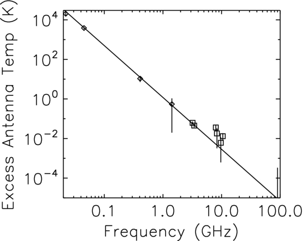
The errors and their correlations in the data are described by the matrix shown in Table 5. Although the covariances are not shown in the plots, they are used in the calculations. The fit is nonlinear so strictly speaking the final uncertainties are not Gaussian. At the solution the fit is not strongly nonlinear so the Gaussian approximation is still valid. However, the selection of the reference frequency, although irrelevant to the final χ2 or model, does affect covariances of the parameters. The correlation between the β uncertainty and the TR uncertainty is strongly affected by the choice of ν0 and the best choice of ν0 depends on the frequencies and uncertainties of the data sets being fit. The details are addressed in the Appendix. We obtain best-fit values T0 = 2.725 ± 0.001 K, TR = 24.1 ± 2.1 K, and β = −2.599 ± 0.036 with χ2 = 17.4, for reference frequency ν0 = 310 MHz and 11 dof. Figure 5 shows the radio background after subtracting off the best-fit CMB temperature. The ARCADE 2 data are in good agreement with the excess radio spectrum derived from the low-frequency surveys.
Figure 5. Excess antenna temperature as a function of frequency. The line is the best-fit line with a −2.6 index. Diamonds are low-frequency points from the literature. Squares are ARCADE 2 data. The 30 GHz data point is included in the fit but since its excess temperature comes out negative it does not appear on the plot. The 90 GHz error bar just appears at the lower right corner of the plot. The covariances are not shown, but they are included in the fit.
Download figure:
Standard image High-resolution image
A χ2 of 17.4 for 11 dof should be expected ∼10% of the time. Most of this excess χ2 is from two points, the 8 GHz low channel and the 30 GHz high channel. If these two points are excised the result is T0 = 2.725 ± 0.001 K, TR = 24.4 ± 2.1 K, and β = −2.595 ± 0.037 with a χ2 of 8.2 for 9 dof. This shows the result does not depend on these two points. We have no a priori reason that these two points should be bad. Further each of the points is only effectively 2σ and in a data set this large one 2σ point should be expected. We thus include all data when fitting for the uniform temperature.
7. DISCUSSION
The ARCADE 2 measurement of the CMB temperature is in agreement with the FIRAS measurement at higher frequencies. The double-nulled design and novel open-aperture cryogenic optics demonstrate significant improvements in both calibration accuracy and control of systematic errors compared to previous measurements at these frequencies. With only 2 hr of balloon flight observations, ARCADE 2 approaches the absolute accuracy of long-duration space missions.
The absolute temperature scale for ARCADE 2 is set by the calibration of thermometers embedded in the external blackbody calibrator, and is cross-checked using observations of the superfluid transition in liquid helium. The largest uncertainties in the ARCADE 2 measurements result from thermal gradients within the blackbody calibrator. These gradients are driven by heat flow from the 2.7 K calibrator through the diffuse helium gas to the colder (1.5 K) aperture plate below. The temperatures within the calibrator are monitored using 21 thermometers suitably spaced to fully sample the calibrator gradient. The gradient is largely confined to the tips of the absorber cones within the calibrator: 97% of the calibrator volume lies within 10 mK of the base temperature. A principal component analysis of the thermometer data demonstrates that the thermal state of the calibrator at any point in time can be characterized using only a few modes formed from linear combinations of the thermometers. The first four modes are clearly related to the expected heat flow from the calibrator to the aperture, and account for 99.98% of the thermometer variance. We conservatively model the calibrator thermal state using the first 10 modes, accounting for 99.996% of the thermal variance. Tests comparing the sky temperature derived after dropping individual thermometers demonstrate that the calibrator has more than enough thermometers to adequately sense the in-flight thermal gradients. In fact, four or five well-placed thermometers would have been sufficient to measure the key thermal gradients within the calibrator.
The 3 GHz radiometer "looks" deeper into the warmer parts of the calibrator. The tips of the calibrator, which are cooler and more variable, are preferentially observed by the higher frequency radiometers. But the higher frequency radiometers are in agreement with the FIRAS results. The lower frequency results (3 and 8 GHz) are corroborated by the low-frequency measurements done entirely independently.
Further improvements in the calibrator performance are possible. For operational simplicity, the instrument design forces the temperature of the aperture plate and horn antennas to the helium bath temperature by flooding reservoirs attached to these structures with superfluid liquid helium. It would be straightforward to modify the thermal design so that the aperture plate and horns are only weakly coupled to the bath, allowing thermal control of these surfaces analogous to the successful calibrator design. Even modest thermal control could reduce the temperature difference between the calibrator and the aperture, thereby reducing heat flow and associated thermal gradients within the calibrator by an order of magnitude or more.
The detected radio background is brighter than expected. Low-frequency Galactic radiation, and by extension extragalactic radiation, is thought to be a mixture of synchrotron and free–free emission. Our analysis shows the detected radio spectrum to be consistent with a single power law with spectral index β = −2.599 ± 0.036 from 22 MHz to 10 GHz. Estimates of radio point sources (Windhorst et al. 1993; Gervasi et al. 2008) indicate a similar spectrum, but the radio background from ARCADE 2 and radio surveys is a factor of ∼6 brighter than the estimated contribution of radio point sources.
It is difficult to reconcile the detected radio spectrum with the contribution from a population of radio point sources (Seiffert et al. 2011). Could the detected signal be in error? The thermal gradient in the ARCADE 2 calibrator is an obvious source of concern for systematic errors. However, the gradient is well sampled and the uncertainties associated with the calibrator thermal state are included in the ARCADE 2 uncertainties. Furthermore, the bulk of the gradient is concentrated at the tips of the cones. The skin depth for absorption within the calibrator is a function of frequency: the high-frequency channels preferentially sample the tips and outer surface of the absorber cones, while the 3 GHz channel samples the entire absorber volume. The results agree within uncertainties with previous measurements at 10 GHz and 30 GHz (Staggs et al. 1996; Fixsen et al. 2004). The agreement between the high-frequency channels and the FIRAS CMB temperature argues against any undetected systematic errors associated with thermal gradients within the calibrator.
Further evidence against an error in the ARCADE 2 data comes from comparing the ARCADE 2 data to a similar analysis using independent radio surveys (Table 4). Repeating the CMB/radio fit from Equation (6) but using various combinations of data yields parameters in Table 6. None of the combinations are in serious disagreement with any of the others. The results do not depend on the assumed and measured relationships among the various data although a full covariance treatment is used to assess the effects of correlated errors. The result is substantially the same if any combination of the low-frequency data points is used (except the 1.42 GHz data alone which do not have a long enough lever arm in frequency to get a good measure of the index), so the result is insensitive to the correlations among the low-frequency measures. The low-frequency data alone measure a large radio excess. The FIRAS data constrain the CMB temperature. The index is constrained with the low-frequency data or the relation of the low-frequency data to the ARCADE 2 data. The ARCADE 2 aid in constraining the amplitude and the index of the radio spectrum. The ARCADE 2 data alone do not have sufficient low-frequency coverage to determine the spectral index of the 3 GHz excess. We assume a spectral index −2.6 and fit the ARCADE 2 data alone for the ARCADE 2 and FIRAS data. The two independent data sets agree on both the CMB temperature and radio amplitude, reducing the likelihood of serious systematic error in either data set.
The ARCADE 2 instrument has clearly shown excess radiation over the CMB at 3 GHz. The excess radio spectrum fits well to a power law. The index is determined by low-frequency measurements outside of ARCADE 2 along with the ARCADE 2 measurements. It does not matter particularly which of these are used. The index is ∼ − 2.6. The amplitude of the excess is determined primarily by the ARCADE 2 data. The CMB temperature is best measured by the FIRAS data but the ARCADE 2 and low-frequency data result in a reasonable measurement. A power-law excess along with the CMB is a good description of the observations.
This research is based upon work supported by the National Aeronautics and Space Administration through the Science Mission Directorate under the Astronomy and Physics Research and Analysis suborbital program. The research described in this paper was carried out in part at the Jet Propulsion Laboratory, California Institute of Technology, under contract with the National Aeronautics and Space Administration. We also thank the interns who worked on this experiment Adam Bushmaker, Jane Cornett, Sarah Fixsen, Luke Lowe, and Alexander Rischard. T.V. acknowledges support from CNPq grants 466184/00-0, 305219-2004-9, and 303637/2007-2-FA, and the technical support from Luiz Reitano. C.A.W. acknowledges support from CNPq grant 307433/2004-8-FA.
APPENDIX
The Galactic modeling process adds correlated uncertainties to the existing uncertainties some of which are correlated. The final Galactic modeling has 60 estimates of the extragalactic radiation over 10 frequencies, three lines of sight, and the two methods. Produced along with this is a 60 × 60 covariance matrix B.
Usually to maximize the utility of the data, one would use a weighted fit with the inverse of the covariance matrix as the weight matrix. However, here the correlations are high and the uncertainties particularly for the low-frequency measurements are only rough estimates. The high correlations push the matrix toward singularity (a perfectly correlated set of measurements would mathematically yield a singular matrix), so we average the data over the three lines of sight and the two methods to get a data vector, D'ν with 10 elements. This is equivalent to multiplying the data vector by a 10 × 60 matrix, C, with six elements of 1/6 in each of the 10 rows. To properly treat the covariance matrix, we multiply it by this matrix on each side to get the corresponding covariance matrix.

Both the data vector and the covariance matrix are augmented with the 29.5, 31, 90, and FIRAS data and uncertainties to generate a data vector, D'', with 14 elements and the corresponding 14 × 14 covariance matrix, V'', shown in Table 5. Although the data shown in Table 5 are given in thermodynamic temperature both the D'' and the V'' we use are in antenna temperature. The 29.5, 31, and 90 GHz data include correlations to the other ARCADE data but they are independent of the low-frequency data. The FIRAS data are fully independent so the corresponding row of the covariance matrix has only the diagonal component.
To perform a fit a subset of data, D (possibly the whole set) is selected and the corresponding rows and columns of the covariance matrix are selected to form the corresponding covariance matrix V.
Then the proper χ2 is calculated and minimized.
where T0, TR, and β are the parameters to be determined, xi = hνi/kT0, and ν0 is the reference frequency.
The fit is nonlinear and can either be done by a simple grid search or by iterative techniques. We have used both methods and they agree with each other.
The uncertainty of the resulting parameters is of course correlated. Furthermore the correlation, particularly between the TR and β parameters is strongly influenced by the selection of the reference frequency, ν0. The correlation is large if the ν0 is far from the center of weight of the data. The ideal ν0 minimizes the correlation between the uncertainty of TR and β. This ν0 is different for each data set but it allows the region of acceptable χ2 to be bounded by an ellipsoid aligned with the principle axis that is smaller than other choices of ν0. The full covariances of the results are in Table 7 for ν0 = 310 GHz.
Table 7. Covariances for the Parameters Given in Table 6
| Covariance | T0T0 | T0β | T0TR | ββ | βTR | TRTR |
|---|---|---|---|---|---|---|
| Data Sets | (mK)2 | (mK) | (mK K) | - | (K) | (K)2 |
| LF+ARC+FR | 0.9420 | −0.0037 | −0.1867 | 0.0013 | 0 | 4.438 |
| LF+ARC | 16.13 | −0.0684 | −10.49 | 0.0017 | 0 | 83.98 |
| LF+FR | 1.0000 | −0.0001 | −0.1172 | 0.0079 | 0.43 | 126900 |
| ARC+FR | 0.9422 | ⋅⋅⋅ | −0.4160 | ⋅⋅⋅ | ⋅⋅⋅ | 9.413 |
| LF | 335500 | −24.48 | −30860 | 0.0097 | 1 | 180200 |
| ARC | 16.31 | ⋅⋅⋅ | −7.178 | ⋅⋅⋅ | ⋅⋅⋅ | 12.39 |
Note. Units are listed at the headings.
Download table as: ASCIITypeset image