


ABSTRACT
New improved empirical calibrations for the determination of electron temperatures and oxygen and nitrogen abundances in H ii regions from the strong emission lines of oxygen, nitrogen, and sulfur are given. They are derived using spectra of H ii regions with measured electron temperatures as calibrating data. Calibration relations are given separately for three classes of H ii regions: cool, warm, and hot ones. Criteria for assigning a H ii region to one of these classes are suggested. We find that classification ambiguities arise only in the case of hot H ii regions with enhanced nitrogen abundances. The derived calibrations provide reliable abundances for H ii regions: the mean difference between oxygen abundances determined from the calibrations and Te-based oxygen abundances is ∼0.075 dex, while it is ∼0.05 dex for nitrogen abundances.
Export citation and abstract BibTeX RIS
1. INTRODUCTION
Accurate metallicities play a key role in many investigations of galaxies. Gas-phase oxygen and nitrogen abundances are broadly used to measure these metallicities. It is believed (e.g., Stasińska 2006) that emission lines due to photoionization by massive stars are the most powerful indicator of the chemical composition of galaxies, both in the low- and intermediate-redshift universe. Accurate oxygen and nitrogen abundances in H ii regions can be derived via the classic Te method, often referred to as the direct method. This method is based on the measurement of the electron temperature t3 within the [O iii] zone and/or the electron temperature t2 within the [O ii] zone. The ratio of the nebular to auroral oxygen line intensities [O iii](λ4959+λ5007)/[O iii]λ4363 is usually used for the t3 determination, while the ratios of the nebular to auroral nitrogen line intensities [N ii](λ6548 + λ6584)/[N ii]λ5755 or [O ii](λ3727 + λ3729)/[O ii](λ7320 + λ7330) are used for the t2 determination. In high-metallicity H ii regions, however, the auroral lines become too faint to be detected.
Pagel et al. (1979) and Alloin et al. (1979) have suggested that the locations of H ii regions in some emission-line diagrams can be calibrated in terms of their oxygen abundances. This approach to abundance determination in H ii regions, usually referred to as the "strong line method," has been widely adopted, especially in the cases where the temperature-sensitive [O iii] λ4363 line is not detected. Numerous relations have been proposed to convert metallicity-sensitive emission-line ratios into metallicity or temperature estimates (e.g., Dopita & Evans 1986; Zaritsky et al. 1994; Vilchez & Esteban 1996; Pilyugin 2000, 2001; Pettini & Pagel 2004; Tremonti et al. 2004; Pilyugin & Thuan 2005; Liang et al. 2006; Stasińska 2006; Thuan et al. 2010). Comparisons between abundances derived from various calibrations are given in the recent papers of Kewley & Ellison (2008) and López-Sánchez & Esteban (2010). The strong-line method relies on the following considerations. The emission line properties of a photoionized H ii region are governed by its heavy element content and the electron temperature distribution within the photoionized nebula. In turn, the latter is controlled by the ionizing star cluster spectral energy distribution and by the chemical composition of the H ii region. The evolution of a giant extragalactic H ii region associated with a star cluster is thus caused by a gradual change over time of the integrated stellar energy distribution due to stellar evolution. This has been the subject of numerous investigations (Stasińska 1978, 1980; McCall et al. 1985; Dopita & Evans 1986; Moy et al. 2001; Stasińska & Izotov 2003; Dopita et al. 2006, among others). The general conclusion of those studies is that H ii regions ionized by star clusters form a well-defined fundamental sequence in different emission-line diagnostic diagrams. That such a fundamental sequence exists is the basis for constructing various relations to convert the strong line fluxes into oxygen abundances.
It should be emphasized that there are two types of calibrations: (1) theoretical calibrations based on photoionization models and (2) empirical calibrations based on H ii regions with measured electron temperatures. The oxygen abundances derived using these calibrations show a large scatter (up to ∼0.6 dex), with theoretical calibrations giving high values and empirical calibrations giving lower ones (Pilyugin 2003; Kewley & Ellison 2008; López-Sánchez & Esteban 2010). Because of the large abundance discrepancies between the different types of calibrations, the question then arises: which type of calibration is most reliable? Stasińska (2004, p. 126) has noted that "a widespread opinion is that photoionization model fitting provides the most accurate abundances. This would be true if the constraints were sufficiently numerous (not only on emission line ratios, but also on the stellar content and on the nebular gas distribution) and if the model fit were perfect (with a photoionization code treating correctly all the relevant physical processes and using accurate atomic data). These conditions are never met in practice." Thus, the statement that H ii region models provide realistic abundances should not be taken for granted.
The classic Te method has been questioned by Peimbert (1967). It is known that metallicities derived from collisionally excited lines of heavy elements in H ii regions are systematically lower than those derived from recombination lines by factors ∼ 2 (Rodríguez & García-Rojas 2010, and references therein). Peimbert et al. (1993) have suggested that these differences can be accounted for by the presence of spatial temperature fluctuations inside H ii regions. This interpretation suggests that the classic Te method based on collisionally excited lines results in overestimated electron temperatures and, consequently, in underestimated element abundances in H ii regions. However, this interpretation meets with several difficulties.
First, Barlow et al. (2003) have found that the recombination line abundance discrepancies appear to be restricted to ions of the second row of the periodic table (carbon, nitrogen, oxygen, and neon) but do not affect third row ions (e.g., magnesium). Nebular temperature fluctuations cannot account for this fact.
Second, Guseva et al. (2006, 2007) have determined for a large sample of H ii regions the temperatures Te(H+) of the H+ zones using the Balmer and Paschen jumps and the temperatures Te([O iii]) of the O++ zones from collisionally excited lines. They found that the Te(H+) and Te([O iii]) temperatures do not differ statistically, although small temperature differences of the order of 3%–5% cannot be ruled out.
Third, oxygen abundances derived with the Te method have been verified by high-precision model-independent determinations of the interstellar oxygen abundance in the solar vicinity, using high-resolution observations of the weak interstellar O iλ1356 absorption line toward stars (see discussion and references in Pilyugin 2003). More recently, Williams et al. (2008) have measured UV resonance line absorptions in the spectra of central stars of planetary nebulae produced by the nebular gas, for the ions that emit optical forbidden lines. They found that the collisionally excited forbidden lines yield column densities that are in basic agreement with the column densities derived for the same ions from the UV absorption lines. Williams et al. (2008) have concluded that the temperatures and abundances based on the forbidden lines are reliable.
Fourth, Bresolin et al. (2009) have shown that the oxygen abundances derived with the Te method in H ii regions of the spiral galaxy NGC 300 agree well with the stellar abundances. They have concluded that the Te-based chemical abundances in extragalactic H ii regions are reliable measures of the nebular abundances.
Thus, there are strong evidences that the metallicity scale defined by the classic Te method is the most reliable one. The discrepancies between metallicities based on the collisionally excited lines and those based on the recombination lines can be caused by errors in the line recombination coefficients by factors of ∼ 2 (Rodríguez & García-Rojas 2010). Therefore, in the following, we will base our calibration relations on H ii regions with electron temperatures obtained with the Te method.
In a number of previous studies (Pilyugin 2000, 2001, 2005; Pilyugin & Thuan 2005; Pilyugin et al. 2009), we have constructed empirical calibrations for the determination of electron temperatures and oxygen abundances using indexes based on the strong oxygen line fluxes. It has been found that those calibrations provide realistic estimates of oxygen abundances, i.e., the combination of the line flux R3 (to be defined below) and of the excitation parameter P = R3/(R3 + R2) is a reliable index of temperature and metallicity. However, those calibrations present two difficulties. First, the relationship between oxygen abundance and strong oxygen line fluxes is double-valued, with two distinct parts usually known as the lower and upper branches of the R23–O/H diagram. Thus, one has to know a priori on which of the two branches the H ii region lies. Second, those calibrations cannot be applied to H ii regions which lie in the transition zone, i.e., with oxygen abundances 8.0 ≲ 12 + log(O/H) ≲ 8.3.
We wish here to construct empirical calibrations that can overcome those difficulties or at least alleviate them. The general strategy of our investigation is the following. We will discuss here only temperature calibrations. However, our arguments are applicable to metallicity calibrations as well, since there is a good correlation between metallicity and electron temperature in H ii regions. Therefore, a reliable temperature index should also be a reliable metallicity index. Pilyugin et al. (2009) found that the temperature-sensitive ratio of nebular to auroral oxygen line intensities [O iii](λ4959+λ5007)/[O iii]λ4363 can be expressed in terms of R3 and P. In other words, the combination of R3 and P can serve as a surrogate temperature index. Unfortunately, this surrogate index does not work in the transition zone. We need then to find one or several other temperature indexes that do so. Moreover, we would expect that empirical calibrations based on two or more indexes of temperature would provide a more reliable estimate of the latter. In order for our calibrations to apply to as many H ii regions as possible, we will consider indexes involving the strong lines of three different elements: oxygen, nitrogen, and sulfur. These have been measured by a number of investigators in the spectra of many H ii regions. They are:
Are there other combinations of the strong lines of oxygen, nitrogen, and sulfur that can be used as reliable temperature indexes? It is generally accepted that the [O ii], [N ii], and [S ii] lines arise at similar temperatures. The energy of the level that gives rise to the R2 line (the [O ii](λ3727+λ3729) doublet) is higher than both the energies of the levels giving rise to the S2 and N2 lines. Thus, the line-emissivity ratios j(N2)/j(R2) and j(S2)/j(R2) are temperature sensitive; they increase with decreasing electron temperature. It should be noted however that these line ratios are not exclusively governed by the dependence of the line emissivities on the electron temperature. In the case of sulfur, one may assume that the S/O abundance ratio is constant in all H ii regions, since sulfur and oxygen are thought to be produced by the same massive stars. However, the S+ zone does not coincide with the O+ zone (Garnett 1992), and their size ratio is thought to depend on the electron temperature. One can then expect that, to first approximation, the S2/R2 ratio depends only on the electron temperature. It can then be used as a surrogate indicator of the electron temperature, although the temperature dependence of S2/R2 = f(t2) is more complex than that of j(S2)/j(R2) = f(t2). In the case of nitrogen, the N+ zone is nearly coincident with the O+ zone. But the N/O abundance ratio is not the same for all H ii regions. At high metallicities, the N/O abundance ratio increases with decreasing electron temperature (i.e., with increasing oxygen abundance). Again, one can expect that, to first approximation, the N2/R2 ratio depends only on electron temperature and can be used as a surrogate indicator of the electron temperature, although the temperature dependence N2/R2 = f(t2) is also more complex than that of j(N2)/j(R2) = f(t2). One can thus expect that both N2/R2 and S2/R2 ratios are reliable temperature indexes.
Calibrations based on oxygen and nitrogen strong lines have been considered in a number of studies. Denicolo et al. (2002) have calibrated the N2 estimator using a compilation of H ii regions with accurate oxygen abundances, in addition to photoionization models. The derived oxygen abundances in individual H ii regions can deviate from their adopted relation by as much as 0.5 dex. Pettini & Pagel (2004) have also constructed a calibration 12 + log(O/H) = f (N2) and found that their O/H estimates have an accuracy of ∼0.4 dex at the 95% confidence level. They have also considered the dependence of R3/N2 index on O/H. Pettini & Pagel (2004) concluded that this index is of little use at low metallicities. However, at moderate-to-high metallicities, greater than ∼1/4 solar, the oxygen abundance can be deduced to within a factor of ∼0.25 dex (at the 95% confidence level) from the 12 + log(O/H) = f (R3/N2) relation. Bresolin (2007) has considered the N2/R2 index as a function of Te, based on oxygen abundances for extragalactic H ii regions. The rms of the fit to these data is ∼ 0.20 dex. Thus, the accuracy of abundance estimates with existing calibrations based on the nitrogen and oxygen strong lines is low. We will show below that, by using calibrations based on several indexes, the accuracy of abundance estimates can be significantly improved.
We discuss the sample of calibrating data points used to establish our calibrations in Section 2. The relations for the determination of electron temperatures and oxygen and nitrogen abundances are derived in Section 3. We discuss our results in Section 4, and present our conclusions in Section 5.
Throughout the paper, the electron temperatures will be given in units of 104 K.
2. SELECTION AND ANALYSIS OF THE CALIBRATING SAMPLE
2.1. A Sample of Calibrating H ii Regions
We wish to assemble here a sample of calibrating H ii regions with metallicities spanning a large range. Spectrophotometric measurements of moderate- and high-metallicity (12 + log(O/H) ≳ 8.0) H ii regions, with accurate measured electron temperatures t3 = t(O iii) or/and t2 = t(N ii), include those of H ii regions in disks of nearby spiral galaxies—NGC 300 (Bresolin et al. 2009), NGC 1365 (Bresolin et al. 2005), NGC 5194 = M 51 (Bresolin et al. 2004; Garnett et al. 2004), NGC 5236 = M 83 (Bresolin et al. 2005), NGC 5457 = M 101 (Esteban et al. 2009; Garnett & Kennicutt 1994; Izotov et al. 2007; Kennicutt et al. 2003; Kinkel & Rosa 1994; Luridiana et al. 2002; McCall et al. 1985; Rayo et al. 1982; Sedwick & Aller 1981; Torres-Peimbert et al. 1989; van Zee et al. 1998)—and in irregular galaxies—NGC 6822 (Hernández-Martínez et al. 2009; Hidalgo-Gámez et al. 2001; Miller 1996; Peimbert et al. 2005) and the Small Magellanic Cloud (SMC; Dufour et al. 1982; Testor 2001; Testor et al. 2003).
To select accurate measurements of H ii regions in spiral galaxies, we require that the deviation of the oxygen abundance of the H ii region from the general linear relation that describes the radial oxygen abundance gradient in the disk to be less than ∼0.1 dex. In the case of the spiral galaxy NGC 1365, the number of H ii regions with a measured electron temperature is too small to establish with certainty the radial distribution of oxygen abundances in the disk (Bresolin et al. 2005). However, the oxygen abundance of H ii region 15, based on the measurement of the electron temperature t(N ii), is confirmed independently by the one based on the measured electron temperature t(S iii), as well as by the abundances of H ii regions 5 and 14, at nearly the same galactocentric distance (Bresolin et al. 2005). Therefore, H ii region 15 in the disk of NGC 1365 has been included in our sample of calibrating H ii regions. As for the dwarf irregular galaxies NGC 6822 and the SMC, since the oxygen abundance is relatively constant over their extent (e.g., Croxall et al. 2009), we have required the deviations of oxygen abundances from the mean value to be less than ∼0.1 dex. Moreover, if temperature estimates from both the [O iii]λ4363 and [N ii]λ5755 auroral lines are available for the same H ii region, they are considered to be independent measurements. Using the above selection criteria, we have selected 72 measurements of moderate- and high-metallicity (12 + log(O/H) ≳ 8.0) H ii regions as calibrating data points. As for low-metallicity (12 + log(O/H) ≲ 8.0) calibrating H ii regions with accurate electron temperature t3, the data (46 data points) have been taken from Izotov et al. (2007). Thus, our calibrating sample contains a total of 118 data points.
To ensure that we have a relatively homogeneous data set, we have recalculated electron temperatures and oxygen and nitrogen abundances for all the calibrating H ii regions, within the framework of the standard H ii region model with two distinct temperature zones within the nebula. The equations used to derive electron temperatures from line fluxes are given in the next section.
2.2. The Te-method Equations
To convert the values of the line fluxes to the electron temperatures t3,O and t2,N and to the ion abundances O++/H+, O+/H+, and N+/H+, we have used the five-level atom model for the O++, O+, and N+ ions, updated by recent atomic data. The Einstein coefficients for the spontaneous transitions Ajk for the five low-lying levels for all ions above have been taken from Froese Fisher & Tachiev (2004). The energy level data are from Edlén (1985) for O++, from Wenåker (1990) for O+, and from Galavís et al. (1997) for N+. The effective cross sections (or effective collision strengths) for electron impact Ωjk as a function of temperature are from Aggarwal & Keenan (1999) for O++, from Pradhan et al. (2006) for O+, and from Hudson & Bell (2005) for N+. To derive the effective cross section for a given electron temperature, we have fitted a second-order polynomial to these data.
In the low density regime (ne ≲ 100 cm−3), the following simple expressions provide approximations to the numerical results with accuracy better than 1%. The electron temperatures are related to the measured line fluxes in the following way:
and
or
where Q3,O = [O iii](λ4959+λ5007)/[O iii]λ4363 is the ratio of nebular to auroral oxygen line intensities in the t3,O zone, Q2,N = [N ii](λ6548 + λ6584)/[N ii]λ5755 is the ratio of nebular to auroral nitrogen line intensities, and Q2,O = [O ii](λ3727 + λ3729)/[O ii](λ7320 + λ7330) is the ratio of nebular to auroral oxygen line intensities in the t2,O zone.
The equations relating ion abundances to measured line fluxes are:
and
The total oxygen abundance is determined from
The total nitrogen abundance is determined from
assuming
The N+/O+ ion abundance ratio is derived from
which is obtained by combining Equation (4) with Equation (5).
The relation between the electron temperatures t2 within the O+ zone and t3 within the O++ zone is

This relation derived by Pilyugin et al. (2009) is very similar to the commonly used ones of Campbell et al. (1986) and Garnett (1992).
2.3. Behavior of the Electron Temperature and Abundance Indicators
Here, we examine how the fluxes and flux ratios of various emission lines in the calibrating H ii regions vary as a function of electron temperature t2 (Figure 1) and of oxygen (Figure 2) and nitrogen (Figure 3) abundances. Inspection of those variations shows that none of the considered emission line fluxes and flux ratios displays a monotonic behavior with electron temperature and oxygen and nitrogen abundances over the whole temperature (or metallicity) range. Instead, the curves show bends. Close examination suggests that there are three distinct regimes, depending on the temperature of the H ii region, i.e., on whether it belongs to the class of cool, warm, or hot H ii regions. We have therefore decided to construct distinct calibrations for the determination of temperature and abundances for each of these classes of H ii regions.
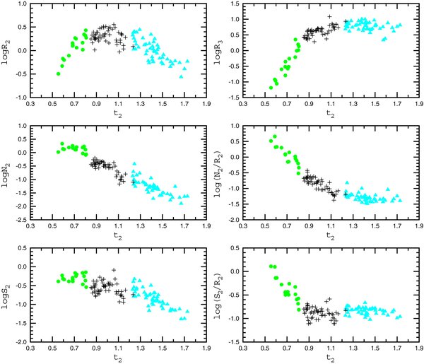
Figure 1. Emission line fluxes and line flux ratios as a function of electron temperature t2 for the sample of calibrating H ii regions. The gray (light green in the online version) filled circles denote cool H ii regions (log N2 > −0.1). The dark (black in the online version) plus signs denote warm H ii regions (log N2 < −0.1 and 12 + log (O/H) > 8.0). The gray (light blue in the online version) filled triangles denote hot H ii regions (12 + log (O/H) < 8.0).
Download figure:
Standard image High-resolution image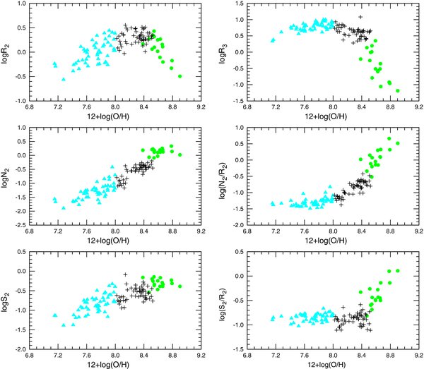
Figure 2. Emission line fluxes and line flux ratios as a function of oxygen abundance 12 + log(O/H) for the sample of calibrating H ii regions. The symbol meaning is the same as in Figure 1.
Download figure:
Standard image High-resolution image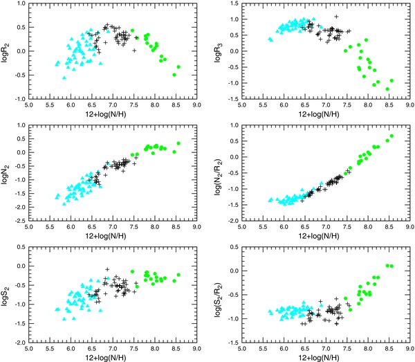
Figure 3. Emission line fluxes and line flux ratios as a function of nitrogen abundance 12 + log(N/H) for the sample of calibrating H ii regions. The symbol meaning is the same as in Figure 1.
Download figure:
Standard image High-resolution imageIn the cool high-metallicity H ii regions, the R2 and R3 line fluxes strongly decrease with decreasing electron temperature, or equivalently, with increasing oxygen and nitrogen abundances. On the contrary, the N2 line fluxes remain approximately constant with temperature, forming a sort of plateau. The behavior difference between the R2 and N2 line fluxes have a natural explanation as the interplay of two factors. On the one hand, the line-emissivity j(R2) is temperature sensitive, i.e., the emissivity decreases with decreasing electron temperature, causing a decrease of the R2 line flux for lower electron temperatures. On the other hand, the oxygen abundance increases on average with decreasing electron temperature, resulting in an increase of the R2 line flux with decreasing electron temperature. The combination of these two factors results in a decrease of the R2 line flux with decreasing electron temperature. Since at 12 + log(O/H) ≳ 8.3, secondary nitrogen becomes dominant and the nitrogen abundance increases at a faster rate than the oxygen abundance (Henry et al. 2000), the change of nitrogen abundances with decreasing electron temperature is larger than that of oxygen abundances and, as a consequence, compensates the decrease of the line-emissivity j(N2). Thus, the N2 line fluxes remain approximately constant in cool H ii regions.
Inspection of Figure 4 shows that cool H ii regions can be selected with the criteria logN2 ≳ −0.1. They are shown in Figures 1, 2, 3, and 4 by the gray (light green in the color online version) filled circles. The adopted boundary between the cool H ii regions and the warm H ii regions is shown by the dotted line in Figure 4. It should be emphasized that the R2, R3 line fluxes and the N2/R2, S2/R2 flux ratios in cool H ii regions are very sensitive to electron temperature and oxygen and nitrogen abundances. One can thus expect these parameters to act as reliable temperature and metallicity indexes.
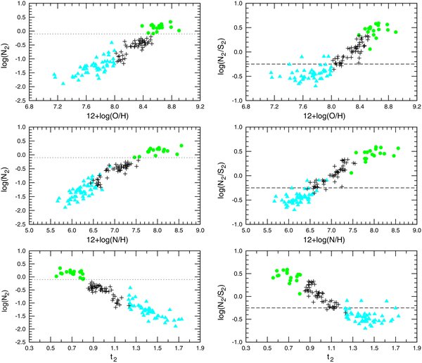
Figure 4. Emission line fluxes N2 and flux ratios N2/S2 as a function of oxygen abundance 12 + log(O/H) (upper panels), nitrogen abundance 12 + log(N/H) (middle panels), and electron temperature t2 (lower panels) for the sample of calibrating H ii regions. The symbol meaning is the same as in Figure 1. The dotted line is the adopted boundary between cool H ii regions and warm H ii regions. The dashed line is the adopted boundary between warm H ii regions and hot H ii regions.
Download figure:
Standard image High-resolution imageClose examination of the behavior of emission line fluxes and flux ratios with electron temperature and oxygen and nitrogen abundances suggests that there is a second bend in the curves at t2 ∼ 1.2 or at 12 + log(O/H) ∼ 8.0, although this bend is less prominent than the previous one. This bend suggests that we should consider separately warm H ii regions with 12 + log(O/H) ≳ 8.0 and hot H ii regions with 12 + log(O/H) ≲ 8.0. The warm H ii regions are shown in Figures 1, 2, 3, and 4 by the dark (black in the color version) plus signs, while the hot ones are shown by the gray (light blue in the online color version) filled triangles. Examination of Figure 4 shows that the value of log(N2/S2) = −0.25 can be taken as indicating roughly the boundary between warm and hot H ii regions, although this criterion is not very precise. Another way for distinguishing between warm and hot H ii regions in disks of spiral galaxies will be discussed below. It should be noted that the strong line fluxes and flux ratios of warm and hot H ii regions are less sensitive to electron temperature and oxygen and nitrogen abundances than those of cool H ii regions.
To summarize, we propose to divide H ii regions into three classes: cool, warm, and hot ones. The adopted classification criteria and parameters of these three H ii region classes are summarized in Table 1. Distinct calibration relations for the determination of temperatures and abundances are derived below for each of these classes.
Table 1. Classification of H ii Regions
| H ii Region | Classification Criteria | Metallicity | Temperature |
|---|---|---|---|
| Class | Range | Range | |
| Cool | log(N2) ⩾ −0.1 | 12 + log(O/H) ≳ 8.4 | 0.85 ≳ t2 |
| Warm | log(N2) < −0.1, log(N2/S2)⩾ −0.25 | 8.55 ≳ 12 + log(O/H) ≳ 8.0 | 1.2 ≳ t2 ≳ 0.85 |
| Hot | log(N2)< −0.1, log(N2/S2) < −0.25 | 8.0 ≳ 12 + log(O/H) | t2≳ 1.2 |
Download table as: ASCIITypeset image
3. TEMPERATURE AND METALLICITY CALIBRATIONS
Within the framework of the standard H ii region model adopted in the present study, the electron temperature in the nebula is characterized by two values, t3 and t2. We will be searching for a calibration to determine t2, which for brevity's sake we will refer to hereafter simply as t. In the case where a measurement of t3 is available for a calibrating H ii region, t2 is derived from Equation (11). We have argued above that log(N2/R2) and log(S2/R2) can serve as a surrogate indicators of t2. At the same time, the combination of P and log R3 can serve as a surrogate indicator of t3. Since there is a one-to-one correspondence between t2 and t3, the same indicators can be used for the determination of both t2 and t3. One can expect from general considerations that it is preferable to construct calibrations based on indexes that reflect the physical conditions of both O+ and O++ zones, especially in the case of metallicity calibrations.
3.1. The ONS Calibration
Here, we search for a calibration that makes use of both N2/R2 and S2/R2 ratios as temperature and metallicity indexes. This calibration will be referred to as the ONS calibration.
3.1.1. Calibration Relations for Temperature
We adopt the following simple expression to relate the electron temperature to the above surrogate indicators:
This expression is analogous to the equation for determining electron temperature in the classic Te method, see Equations (1) and (2). The numerical values of the coefficients in Equation (12) can be derived from the condition that the scatter of the residuals σt defined as
is minimal. Here, tCALj is the electron temperature t2 calculated from Equation (12) and tOBSj is the measured t2. With this requirement, we have derived the following relations for the determination of the electron temperature:
The quantity tONS denotes here the electron temperature t2 derived from the calibration relation.
3.1.2. Calibration Relations for Oxygen and Nitrogen Abundances
As discussed above, the combination of these parameters can also serve as an indicator of the oxygen abundance in cool H ii regions. The following simple expression
is adopted to relate the oxygen abundance to the strong line fluxes. Again, the numerical values of the coefficients in Equation (15) can be derived from the requirement that the scatter of the residuals σO/H defined as
is minimal. Here, (O/H)CALj is the oxygen abundance calculated from Equation (15) and (O/H)OBSj is the measured Te-based oxygen abundance.
The relations
have been obtained. A few points show large (>0.2 dex) deviations. These points have been excluded in deriving the final calibration relations.
In the same way, calibration relations for nitrogen abundance determination in H ii regions have been constructed:
Again, a few points with large (>0.2 dex) deviations have been excluded in deriving the final calibration relations.
3.2. The ON Calibration
In the previous section, we have derived the ONS calibration, using both N2/R2 and S2/R2 ratios as temperature and metallicity indexes. The question arises then whether a calibration, where only one ratio is used as a temperature and metallicity index, can provide reliable estimates of oxygen and nitrogen abundances in H ii regions as well. We have considered the ON calibration based on the N2/R2 ratio and the OS calibration based on the S2/R2 ratio. We found that the accuracies of the oxygen and nitrogen abundances and of the electron temperatures obtained with the ON calibration are comparable with those of the same quantities determined with the ONS calibration, for all classes of H ii regions. On the other hand, the OS calibration provides reliable estimates for some characteristics of H ii regions, such as oxygen abundances in cool H ii regions, but somewhat less reliable estimates of other characteristics, such as nitrogen abundances in warm H ii regions. Thus, we will give only the ON calibration relations below and will not discuss further the OS calibration.
We have derived the following relations for the determinations of the electron temperature tON = t2, of the oxygen abundance 12 + log(O/H)ON, and of the nitrogen abundance 12 + log(N/H)ON:
Again, a few points with large deviations were excluded in the final derivation of the calibration relations.
4. DISCUSSION
We next discuss the reliability of the temperatures and abundances derived with our calibrations.
4.1. Comparison of Observed and Calibration-determined Temperatures and Abundances
The filled gray (light blue in the online version) circles in Figure 5 show the comparison between ONS-calibration-determined (upper panel) and ON-calibration-determined (lower panel) electron temperatures with measured ones in the calibrating H ii regions. Three hot H ii regions (HS 0837+4717, HS 1028+3843, and UM 420), represented by plus signs, show large deviations from the equality solid line. These outliers show significantly enhanced nitrogen line intensities and enhanced N/O ratios. López-Sánchez & Esteban (2010) have found that Wolf-Rayet features are detected in all galaxies with a high N/O ratio. They suggest that it is the ejecta of Wolf-Rayet stars that locally enrich the interstellar medium of these galaxies in nitrogen. López-Sánchez et al. (2007) have quantitatively analyzed the effect of local enrichment in the blue compact dwarf galaxy NGC 5253. They found that the enrichment pattern agrees with that expected for local pollution by the ejecta of Wolf-Rayet stars. Pustilnik et al. (2004) have found that the number of Wolf-Rayet stars in the region of the current starburst in HS 0837+4717 is about 1000. It is not clear however whether Wolf-Rayet ejecta can enhance nitrogen by as much as a factor of 2–3, as is observed. More data are needed to know with more certainty what makes these three galaxies to be outliers. It should be noted that galaxies with significantly enhanced nitrogen abundances are very rare (Pustilnik et al. 2004; López-Sánchez & Esteban 2010). Because of their nitrogen enhancement, the three galaxies HS 0837+4717, HS 1028+3843, and UM 420 have been misclassified as warm H ii regions according to our criteria, while they should have been classified as hot H ii regions. The filled dark squares in Figure 5 show electron temperatures calculated using the calibration for hot H ii regions. It can be seen that the deviations become considerably smaller.
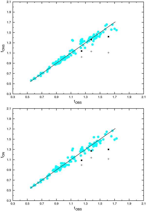
Figure 5. Upper panel: Gray (light blue in the online version) filled circles show the comparison between electron temperatures determined from the ONS calibration and measured temperatures in the calibrating H ii regions. The plus signs show the electron temperatures, determined with the calibration for warm H ii regions, of three hot H ii regions with enhanced nitrogen abundances, misclassified as warm H ii regions according to our classification criteria. The filled dark squares show the electron temperatures in these peculiar H ii regions determined with the calibration for hot H ii regions. The solid line is that of equal values. Lower panel: the same as in the upper panel but for the ON calibration.
Download figure:
Standard image High-resolution imageInspection of Figure 5 shows that the scatter in the tONS–tOBS and tON–tOBS diagrams is smaller for cool H ii regions than that for hot ones. This is not surprising since it has been noted above that our temperature indexes are more sensitive to the electron temperature in cool H ii regions than in warm and hot ones (Figure 1). The rms deviations of electron temperatures for the 115 calibrating H ii regions, excluding the three peculiar objects, are equal  =
=  = 0.054.
We next compare the abundances determined from the calibrations with Te-based abundances. In the upper left panel of Figure 6, we plot the oxygen abundances (O/H)ONS obtained from Equation (17) against the Te-based oxygen abundances. Each calibrating H ii region is represented by a gray (light blue in the online version) filled circle. Equality is shown by the solid line. As before, the plus signs show oxygen abundances in the three peculiar misclassified hot H ii regions determined with the calibration for warm H ii regions, while the filled dark squares show abundances in the same objects determined with the calibration for hot H ii regions. Again, the deviations from the equality line are considerably smaller for the latter. The rms deviation of oxygen abundances for the 115 calibrating H ii regions, excluding the three peculiar objects, is  = 0.074.
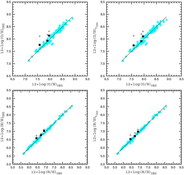
Figure 6. Gray (light blue in the online version) filled circles show the comparison between abundances determined from the ONS calibration and Te-based abundances in the calibrating H ii regions. The plus signs show the abundances, determined with the calibration for warm H ii regions, of three hot H ii regions with enhanced nitrogen abundances, misclassified as warm H ii regions according to our classification criteria. The filled dark squares show the abundances in these peculiar H ii regions determined with the calibration for hot H ii regions. The solid line is that of equal values.
Download figure:
Standard image High-resolution imageIn the upper right panel of Figure 6, we plot the oxygen abundances (O/H) obtained by the Te method equations (Section 2.2) and with electron temperatures t2 estimated from Equation (14), against the Te-based oxygen abundances. The general behavior of the (O/H)
 abundances is similar to that of the (O/H)ONS abundances. The rms deviation of (O/H)
 abundances for the 115 calibrating H ii regions (excluding again the three peculiar objects) is
  = 0.075. It may be surprising that the scatter of the (O/H)
 abundances is not appreciably smaller in the cool H ii regions than in the warm and hot H ii regions since, as discussed before, the scatter in the tONS–tOBS diagram is significantly smaller for cool H ii regions as compared with warm and hot H ii regions. Examination of the equations of the Te method for the determination of oxygen ionic abundances (see Equations (5) and (6)) gives a natural explanation for this apparent inconsistency. Since the oxygen ionic abundance varies in inverse proportion to the electron temperature, the smaller errors in the electron temperatures for H ii regions with t ∼ 0.6 and the twice as larger errors in the electron temperatures for H ii regions with t ∼ 1.2 result in similar errors in the oxygen abundance. Therefore, the smaller scatter in the tONS–tOBS diagram for cool H ii regions does not result in a smaller scatter in the (O/H)
 –(O/H)
 diagram for the same cool H ii regions.
The gray (light blue in the online version) filled circles in the lower left panel of Figure 6 show the nitrogen abundances (N/H)ONS obtained from Equation (18) against the Te-based nitrogen abundances for all the calibrating H ii regions. As before, the solid line shows equality, the plus signs the nitrogen abundances in the three peculiar misclassified hot H ii regions determined with the calibration for warm H ii regions, and the filled dark squares the abundances in these peculiar objects determined with the calibration for hot H ii regions. The rms deviation of nitrogen abundances for the 115 calibrating H ii regions is  = 0.047. Finally, in the lower right panel we plot the nitrogen abundances (N/H)
 against the Te-based nitrogen abundances. The general behavior of the (N/H)
 abundances is similar to that for (N/H)ONS abundances. The rms deviation of (N/H)
 abundances for the 115 calibrating H ii regions is
  = 0.049. It should be emphasized that the calibrations for nitrogen provide more accurate abundances than those for oxygen.
Figure 7 shows the comparison of observed and ON-calibration-determined abundances. Comparison of Figures 6 and 7 shows that the general behavior of the ONS-calibration-determined and the ON-calibration-determined abundances are similar. Direct comparison in Figure 8 of ONS-calibration-determined and ON-calibration-determined abundances and temperatures shows that they are very close to each other.

Figure 7. Same as Figure 6, but for the ON calibration.
Download figure:
Standard image High-resolution image
Figure 8. Gray (light blue in the online version) filled circles show the comparison between oxygen abundances (upper panel), nitrogen abundances (middle panel), and temperatures (lower panel) determined from the ONS calibration and from the ON calibration. The solid line is that of equal values.
Download figure:
Standard image High-resolution imageIn conclusion, the small scatter in Figures 5–7 constitutes evidence that our criteria for selecting calibrating H ii regions with accurate measurements are sound, and that our proposed temperature and metallicity indexes are reliable.
4.2. The O/H–N/O Diagram
Analysis of the O/H–N/O diagram provides another means for checking the reliability of our calibrations. Moreover, this diagram provides a way to evaluate the credibility of abundances determinations in H ii regions where abundances cannot be derived by direct methods. The O/H–N/O diagram is shown in Figure 9. The dark filled circles show the Te-based oxygen and nitrogen abundances in the calibrating H ii regions. The gray (light blue in the online version) filled circles in the upper panel show (O/H)ONS versus (N/H)ONS abundances for the 118 calibrating H ii regions and 411 H ii regions in nearby spiral and irregular galaxies taken from van Zee et al. (1998), van Zee & Haynes (2006), Bresolin et al. (1999), and Bresolin et al. (2005). The plus signs represent again the three peculiar misclassified hot H ii regions with abundances determined with the calibration for warm H ii regions, and the open squares represent the abundances of those objects determined with the calibration for hot H ii regions. We see that the H ii regions with abundances derived with our calibrations and those with Te-based abundances lie in the same general region in the O/H–N/O diagram. In the lower panel, we plot the (O/H)ON and (N/H)ON abundances for the same H ii regions. The general trends in the lower panel are the same as those in the upper panel. The overlap of the dark and gray points is a testimony to the reliability of our calibrations.
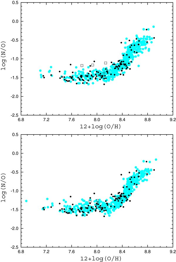
Figure 9. O/H–N/O diagram. Upper panel: the dark filled circles show the Te-based oxygen and nitrogen abundances in the calibrating H ii regions. The gray (light blue in the online version) filled circles show (O/H)ONS and (N/H)ONS abundances of the calibrating H ii regions and of H ii regions in nearby spiral and irregular galaxies from van Zee et al. (1998), van Zee & Haynes (2006), Bresolin et al. (1999), and Bresolin et al. (2005). The plus signs show abundances in three peculiar misclassified hot H ii regions determined with the calibration for warm H ii regions. The open squares show abundances in these peculiar H ii regions determined with the calibration for hot H ii regions. Lower panel: the same as in the upper panel, but for (O/H)ON and (N/H)ON abundances.
Download figure:
Standard image High-resolution image4.3. The Oxygen Abundance Gradient in the Spiral Galaxy M 101
The radial distribution of oxygen abundances in the disk of the spiral galaxy M 101, determined with the Te method, provides us with one more possibility for checking the credibility of our calibrations. It has long been known that the disks of spiral galaxies show radial abundance gradients, with the oxygen abundance being higher in the central part of the disk and decreasing outward. There exists a reliable way to distinguish between hot and warm H ii regions in the disks of spiral galaxies (Pilyugin et al. 2004): move outward from the central part of the disk until the oxygen abundance decreases to 12 + log(O/H) = 8.0, then define the galactocentric radius where that happens to be R*G. Then, the abundances in H ii regions beyond R*G are determined with the calibration for hot H ii regions, and those in H ii regions closer than R*G with the calibration for warm H ii regions. In the case of M 101, R*G is equal to ∼ 0.9R25, where R25 is the isophotal radius at the surface brightness of B = 25 mag arcsec−2. The sources of the spectrophotometric measurements of H ii regions in the disk of M 101 are given in Section 2.1.
The upper panel of Figure 10 shows the radial distribution of oxygen abundances in the disk as determined by the Te method. The linear least-square best fit to those data is shown by the solid line in all three panels of Figure 10. The middle panel shows the radial distribution of (O/H)ONS abundances, and the lower panel that of (O/H)ON abundances. Here, we have used the criteria listed in Table 1 to assign each H ii region to one of three classes. Inspection of Figure 10 shows that all three abundance radial distributions are in good agreement. This is a testimony to the reliability of our calibrations and of our H ii region classification criteria.
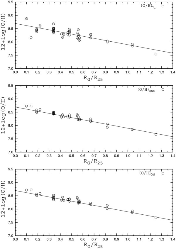
Figure 10. Radial distributions of oxygen abundances in the disk of the spiral galaxy M 101 determined in different ways. Upper panel: the radial distribution of (O/H) abundances. The solid line is the linear least-square best fit to the data. Middle panel: the radial distributions of (O/H)ONS abundances. The solid line is the same as in the upper panel. Lower panel: the radial distribution of (O/H)ON abundances. The solid line is the same as in the upper panel.
Download figure:
Standard image High-resolution image4.4. Comparison with Previous Calibrations
We now compare our calibrations with some previous calibrations. For the sake of definiteness, we will discuss the ONS calibration. López-Sánchez & Esteban (2010) have recently compared the abundances obtained by the Te-method with those derived from previous calibrations. Those authors found the parametric or P calibration (the most recent version being that of Pilyugin & Thuan 2005) to yield the most accurate abundances. We have thus limited ourselves to comparing the oxygen abundances derived from the present calibrations to those obtained from the parametric calibration and from the often-used calibrations of Tremonti et al. (2004):

and of Kobulnicky & Kewley (2004):
where x = logR23 and y = log(R3/R2).
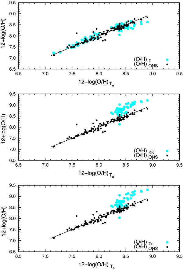
In each panel of Figure 11, we show by dark (black in the color version) circles the oxygen abundances determined with the ONS calibration against the Te-based abundances in the calibrating H ii regions. For comparison, we show with gray (light blue in the color version) circles the (O/H)P abundances estimated with the parametric calibration of Pilyugin & Thuan (2005; upper panel), the (O/H)KK abundances obtained with the calibration of Kobulnicky & Kewley (2004; middle panel), and the (O/H)Tr abundances determined with the calibration of Tremonti et al. (2004; lower panel) against those obtained by the Te method. The solid line shows equality.
Figure 11. Comparison of oxygen abundances determined by the ONS calibration with abundances obtained by some previous calibrations. The (O/H)ONS abundances, the (O/H)P abundances (derived with the most recent parametric calibration of Pilyugin & Thuan 2005), the (O/H)KK abundances (obtained with the calibration of Kobulnicky & Kewley 2004), and the (O/H)Tr abundances (determined with the calibration of Tremonti et al. 2004) are plotted against the Te-based oxygen abundances for the calibrating H ii regions. The solid line shows equality.
Download figure:
Standard image High-resolution image
The upper panel shows that there is a general good agreement between  and (O/H)P abundances. This was also found by López-Sánchez & Esteban (2010). However, the current calibration has several advantages over the P calibration. First, it provides more accurate oxygen abundances, especially in the high-metallicity range. Second, the current calibration is valid over the whole range of metallicity while the parametric calibration is not valid for H ii regions in the transition zone, with 8.0 ≲ 12 + log(O/H) ≲ 8.3. Third, for a correct application of the P calibration, one needs to know a priori on which of the two branches the H ii region lies. In the case of the current calibration, this difficulty arises only for hot low-metallicity H ii regions with enhanced nitrogen abundances. However this difficulty can usually be overcome. Indeed, the auroral line [O iii]λ4363 is often detected in these objects, i.e., a direct measurement of the electron temperature is usually possible. Furthermore, in some types of investigations (for example, the study of radial abundance gradients in the disks of spiral galaxies), there usually exist additional data that help to bypass the difficulty. Finally, this does not happen often as nitrogen-enhanced low-metallicity galaxies are very rare (Pustilnik et al. 2004; López-Sánchez & Esteban 2010).
The middle and lower panels of Figure 11 show that the (O/H)KK and the (O/H)Tr abundances are shifted toward higher values relative to the Te-based abundances. We have also computed (O/H)KK and (O/H)Tr abundances for the H ii regions in M 101 and have found that a similar shift occurs in Figure 10. This shift is not surprising since Tremonti et al. (2004) have noted themselves that their calibration may systematically overestimate oxygen abundances by as much as a factor of two.
Thus, we have shown that the present calibrations yield several advantages over previous ones. They give reliable and improved estimates of electron temperatures and oxygen and nitrogen abundances in H ii regions. To refine the values of the coefficients in the derived calibrations, as well as the dividing boundaries between cool, warm, and hot H ii regions, we need to have a larger sample of high-precision spectrophotometric measurements of H ii regions with fluxes of the auroral oxygen [O iii]λ4363 and/or nitrogen [N ii]λ5755 lines.
5. CONCLUSIONS
New empirical relations for the determination of electron temperatures t2 and oxygen and nitrogen abundances in H ii regions from strong lines of oxygen, nitrogen, and sulfur have been derived. Those relations have been derived using a set of calibrating H ii regions with measured electron temperatures t3 (i.e., with a detected auroral [O iii]λ4363 line) and/or with measured electron temperatures t2 (i.e., with a detected auroral [N ii]λ5755 line).
We suggest a division of H ii regions into three distinct classes: cool (with logN2 ⩾ −0.1), warm (with logN2 < −0.1 and log(N2/S2) ⩾ −0.25), and hot (with logN2 < −0.1 and log(N2/S2) < −0.25) ones. These classification criteria work well except in the case of hot H ii regions with enhanced nitrogen abundances. However, these objects are very rare. Moreover, the auroral [O iii]λ4363 line is usually detected in them, allowing the direct determination of electron temperatures. Also, in some types of studies, additional data usually exist that help to determine abundances in another way.
Separate calibration relations have been constructed for each class of H ii region. The derived relations provide reliable abundances in H ii regions: the root mean square difference between oxygen abundances determined from the present calibration and Te-based oxygen abundances is ∼0.075 dex, while that for nitrogen abundances is ∼0.05 dex. Thus, the suggested calibration provides significantly more accurate oxygen abundances in comparison to existing calibrations. They also give accurate nitrogen abundances and electron temperatures t2.
We are grateful to the referee for constructive comments. J.M.V. and L.S.P. acknowledge the partial support of AYA2007-67965-C03-02 from the Spanish PNAYA and CSD2006-00070 from CONSOLIDER 2010 programme of MICINN. L.S.P. thanks the partial support of the Cosmomicrophysics project of the National Academy of Sciences of Ukraine. T.X.T. is grateful to the support of NASA and NSF.