


ABSTRACT
The masses of coronal mass ejections (CMEs) have traditionally been determined from white-light coronagraphs (based on Thomson scattering of electrons), as well as from extreme ultraviolet (EUV) dimming observed with one spacecraft. Here we develop an improved method of measuring CME masses based on EUV dimming observed with the dual STEREO/EUVI spacecraft in multiple temperature filters that includes three-dimensional volume and density modeling in the dimming region and background corona. As a test, we investigate eight CME events with previous mass determinations from STEREO/COR2, of which six cases are reliably detected with the Extreme Ultraviolet Imager (EUVI) using our automated multi-wavelength detection code. We find CME masses in the range of mCME = (2–7) × 1015 g. The agreement between the two EUVI/A and B spacecraft is mA/mB = 1.3 ± 0.6 and the consistency with white-light measurements by COR2 is mEUVI/mCOR2 = 1.1 ± 0.3. The consistency between EUVI and COR2 implies no significant mass backflows (or inflows) at r < 4 R☉ and adequate temperature coverage for the bulk of the CME mass in the range of T ≈ 0.5–3.0 MK. The temporal evolution of the EUV dimming allows us to also model the evolution of the CME density ne(t), volume V(t), height-time h(t), and propagation speed v(t) in terms of an adiabatically expanding self-similar geometry. We determine e-folding EUV dimming times of tD = 1.3 ± 1.4 hr. We test the adiabatic expansion model in terms of the predicted detection delay (Δt ≈ 0.7 hr) between EUVI and COR2 for the fastest CME event (2008 March 25) and find good agreement with the observed delay (Δt ≈ 0.8 hr).
Export citation and abstract BibTeX RIS
1. INTRODUCTION
The mass m and speed v(t) of a coronal mass ejection (CME) are necessary parameters to determine the kinetic energy  and momentum p(t) = mv(t) of a CME, which provide us fundamental information on the overall energetics and dynamics of the magnetic instabilities that cause solar flares and CMEs. CMEs typically carry a mass in the range of mCME ≈ 1014–1016 g (e.g., Jackson & Hildner 1978; Howard et al. 1985; Vourlidas et al. 2000, 2002; Harrison et al. 2003; Subramanian & Vourlidas 2007), which corresponds to an average mass loss rate of mCME/(Δt · 4πR2☉) ≈ 2 × 10⁻¹⁴–2 × 10⁻¹² (g cm−2 s−1), amounting to ≲1% of the solar wind loss rate in coronal holes, and to ≲10% in active regions, based on an average occurrence of Δt ≈ 1 CME day−1. A typical active region with a size of L ≈ 1010 cm, a base density of ne ≈ 109 cm−3, and a density scale height of λT ≈ 5 × 109 cm (at T ≈ 1.0 MK) has a total mass of mAR ≈ mpneV ≈ mpneL2λT ≈ 1015 g, which is commensurable with the mass of an average CME. The launch of a CME therefore can blow out the major part of an active region, clearing out a dark evacuation corridor in the corona that is manifested as extreme ultraviolet (EUV) dimming, essentially creating a "transient coronal hole" (e.g., Rust & Hildner 1976; Rust 1983), most dramatically seen in soft X-rays (e.g., Hudson & Webb 1997; Sterling & Hudson 1997).
Masses of CMEs have traditionally been determined from coronagraph observations in white light. The CME mass is estimated by subtracting a pre-event image and assuming that the remaining excess brightness Iobs is due to Thomson scattering Ie(ϑ) by electrons at an angle ϑ from the plane of the sky (Minnaert 1930; van de Hulst 1950; Jackson 1962; Billings 1966; Poland et al. 1981; Vourlidas & Howard 2006). Assuming a standard abundance of fully ionized hydrogen with 10% helium, the CME mass is
Usually, the calculations assume ϑ = 0 (all electrons are in the plane of sky), which leads to a minimum value of the CME mass. The CME mass is typically underestimated by a factor of 2 for most cases. The masses of CMEs were measured with Skylab for 21 events in the range of mCME ≈ (0.8–7.9) × 1015 g (Jackson & Hildner 1978), with the Solwind coronagraph during 1979–1981 with an average of mCME = 4.1 × 10¹⁵ g (Howard et al. 1985), and with the SOHO/LASCO coronagraph with an average of mCME = 1.7 × 10¹⁵ g (Vourlidas et al. 2000, 2002), covering a range of mCME ≈ 1015–1016 g (Subramanian & Vourlidas 2007).
Only recently, when STEREO coronagraph observations became available, the three-dimensional (3D) propagation direction could be pinpointed, and an improved CME mass could be evaluated (Colaninno & Vourlidas 2009). Improved CME masses in the order of mCME ≈ (2.6–7.7) × 1015 g were determined from the STEREO/A and B COR2 instruments. The CME is detected in the COR2 field of view about 1–4 hr later after launch from the coronal base, and the improved mass was found to increase with time, asymptotically approaching a constant value after the CME mass emerged out of the occulted area at r ⩽ 4 R☉, and thus verifying the original LASCO observations (Vourlidas et al. 2000). However, it is not known what percentage of the CME mass originates in the low corona compared to the total white light mass. It is, therefore, desirable to develop complementary methods to reliably estimate the amount of mass ejected from below the coronagraph occulter cutoff.
Here we develop and explore a new method of determining CME masses based on EUV observations, using the STEREO/A and B Extreme Ultraviolet Imager (EUVI) instruments (Howard et al. 2008; Wuelser et al. 2004), as illustrated in Figure 1. Some estimates of CME masses based on EUV dimming were previously reported based on SOHO/CDS data (Harrison & Lyons 2000; Harrison et al. 2003) or SOHO/EIT data (e.g., Zhukov & Auchere 2004), but here we develop a fully automated multi-wavelength code and provide a detailed description of it. The (optically thin) EUV emission is proportional to the volume and squared density of the coronal plasma. When a CME is launched, a fraction of the coronal plasma is ejected and clears the field-of-view, leaving a deficit of EUV emission behind that is proportional to the volume and squared (average) density of the ejected CME plasma, called EUV dimming. Our method essentially determines the geometry and volume of the coronal plasma where EUV dimming is detected and calculates the total mass of the plasma that is missing after a CME launch. Applying this method to both STEREO/A and B data, we obtain two independent mass values from two different aspect angles, whose difference yields a realistic absolute error of the method. Choosing CME events that have already been measured with white light coronagraphs, moreover provides an excellent validation of the new method.
Figure 1. Schematic of CME mass determination methods in EUV vs. white light (WL). Using the EUV method, the CME mass is calculated from the missing mass that causes the EUV dimming in the lower corona at r ≲ 1.1 R☉, while the WL method measures the excess of brightness in a coronagraph image, e.g., at r ≳ 4 R☉ beyond the occulting disk of the STEREO/COR2 instrument. In comparison, STEREO/EUVI has a field-of-view of 1.6 R☉.
Download figure:
Standard image High-resolution imageIn Section 2, we describe the data analysis and modeling step by step, applied to STEREO/EUVI A and B data of eight CME events, previously also measured with STEREO/COR2 (Colaninno & Vourlidas 2009). In Section 3, we discuss the new results in the context of previous studies, and in Section 4 we summarize the conclusions.
2. DATA ANALYSIS AND MODELING
2.1. Selection of Events
We start with the eight CME events analyzed in Colaninno & Vourlidas (2009), which have been detected with the STEREO/A and B spacecraft, once they entered the r>4 R☉ field of view of the COR2 coronagraphs. We detect CME-associated EUV dimmings with the EUVI telescopes in six out of these eight CME events defined by COR2, preceding the detection in COR2 by several hours. The events 4 and 5 did not exhibit an associated dimming that could reliably be detected by EUVI, and thus are dropped from further analysis. We analyze EUVI data in time intervals of 3–5 hr before appearance in the COR2 instrument. The analyzed EUVI time intervals, the starting times of EUV dimming observed with EUVI, the flare starting times observed with GOES and RHESSI, the initiation times extrapolated from linear height-time plots of COR2, and the CME appearance times in both COR2/A and B fields are listed in Table 1. The two STEREO spacecraft had separation angles in the range of αsep ≈ 41°–50° during the time period of the 8 selected events between 2007 December and 2008 April.
Table 1. Observational Parameters of Eight Analyzed Flare/CME Events
| Events | 1 | 2 | 3 | 6 | 7 | 8 |
|---|---|---|---|---|---|---|
| Date | 2007 Dec 4 | 2007 Dec 31 | 2008 Jan 2 | 2008 Mar 25 | 2008 Apr 5 | 2008 Apr 26 |
| GOES flare class | ... | C8.3 | C1 | M1.7 | A5 | B6 |
| NOAA active region | 10975 (?) | 10980 | 10980 | 10989 | 10987 | AR/no number |
| STEREO separation | 41 16 16 |
4397 |
4407 |
4717 |
4783 |
4951 |
| EUVI analyzed interval | 03:00–07:00 | 00:00–04:00 | 06:00–11:00 | 18:00–20:30 | 15:00–17:00 | 12:00–15:00 |
| EUVI/A/195 start time | 03:23 | 00:23 | 08:04 | 18:38 | 15:31 | 12:41 |
| EUVI/B/195 start time | 03:24 | 00:38 | 07:26 | 18:27 | 15:22 | 12:58 |
| GOES start time | ... | 00:37 | 06:05 | 18:26 | 15:30 | 13:58 |
| RHESSI start time | ... | 00:01 | ... | 18:44 | 15:37 | 13:29 |
| CME initiation COR2/A | 04:24 | 00:19 | 09:38 | 18:19 | 15:31 | 13:25 |
| CME initiation COR2/B | 04:14 | 00:14 | 09:12 | 18:33 | 15:32 | 13:31 |
| Appearance COR2/A+B | 07:08 | 01:22 | 10:22 | 19:22 | 16:22 | 15:07 |
| COR2–EUVI/A/195 delay | +4.3 hr | +0.7 hr | +3.9 hr | +0.8 hr | +1.0 hr | +2.5 hr |
| Longitude l (NOAA,AR) | 115° (?) | −90° | −71° | −81° | 116° | ... |
| Longitude l (COR2,mass) | 68° | −100° | −64° | −78° | 117° | −48° |
| Longitude l (COR2,model) | 68° | −95° | −56° | −83° | 116° | −21° |
| Longitude l (EUVI,stereo) | ... | ... | −64° ± 4° | ... | ... | −7° ± 2° |
| Longitude l (EUVI,model) | 100° ± 2° | −94° | −72° ± 6° | −85° ± 1° | 107° ± 1° | −9° ± 4° |
| Latitude b (EUVI,stereo) | ... | ... | −14° ± 2° | ... | ... | 15° ± 2° |
| Latitude b (EUVI,model) | −13° | −13° ± 2° | −8° ± 3° | −13° ± 3° | −7° ± 1° | 10° ± 2° |
| Altitude h (EUVI,stereo) | ... | ... | 10 ± 3 Mm | ... | ... | 65 ± 56 Mm |
| Altitude h (EUVI,limb) | 23 ± 1 Mm | 48 ± 27 Mm | ... | 43 ± 1 Mm | 60 ± 10 Mm | ... |
Download table as: ASCIITypeset image
2.2. Localization of EUV Dimming Events
Because the selection of CME events was done with COR2 at a (projected) distance of more than 4 solar radii away from the Sun, the localization of corresponding EUV dimming events down in the lower corona at altitudes of ≲0.1 solar radius is not always unambiguous, in particular when multiple CMEs or flares are fired in rapid succession. Moreover, the visible area on the Sun is different for each STEREO spacecraft and from Earth (or the Earth-orbiting spacecraft RHESSI and GOES).
The first localization method with COR2 is based on the ratio of CME masses determined from the total brightness images of COR2/A and B, which yields the direction and improved mass of CMEs as described in Colaninno & Vourlidas (2009). The so-obtained longitudinal directions (see Table 1 in Colaninno & Vourlidas 2009) are listed in our Table 1 (COR2,mass). A second method based on COR2 data was carried out by forward modeling of a flux-rope model by Thernisien et al. (2009), which yields longitudinal directions that are also quoted in Table 1 of Colaninno & Vourlidas (2009) and listed in our Table 1 (COR2,model). Note that both methods determine the longitudinal direction 4 solar radii away from the Sun and thus do not necessarily need to coincide with the heliographic longitude of the source region.
Determining the CME source location with EUVI data can be accomplished by measuring the centroid position of the strongest EUV dimming in EUVI/A and B. If the source location is visible by both spacecraft, confined to the range of ≈±70 longitude from central meridian, we can use a stereoscopic 3D reconstruction method. This is only feasible for events 3 and 8. For these events, we determine the source locations with stereoscopic triangulation of the EUV dimming centroids (for a description of the method see Figure 4 in Aschwanden et al. 2008 and Figure 5 in Aschwanden 2009). All other events are partially occulted for at least one of the STEREO spacecraft, and thus stereoscopic triangulation is not a reliable method, because the centroid of CME dimming is shifted to higher altitudes above the occulting edge. In those cases, it is more reliable to use only the position measurement from the spacecraft that observes the source closer to disk center, and to assume a height corresponding to a half thermal density scale height for the centroid of the dimming region, Events 1, 2, 6, and 7 occur near the limb, and we can measure the altitude of the centroid of EUV dimming directly, which indeed cover a similar altitude range of h(EUVI, limb) ≈ 20–60 Mm (see Table 1). Correcting for this EUV altitude, we determine the heliographic longitudes of the events 1, 2, 6, and 7. The obtained longitudes l (EUVI,model) and latitudes b (EUVI,model) (see Table 1) agree with the CME directions derived from COR2 or with the active region positions (NOAA AR) (see Table 1) within a few degrees, which corroborates the correct association of EUVI dimmings with COR2 detections of CMEs.
Regarding the association of the CME source regions with NOAA active regions (NOAA ARs), we identified NOAA-numbered active regions without ambiguity in four events (2, 3, 6, 7), and with a spotless active region that is not numbered by NOAA, but clearly visible in EUV in one other case (8). The remaining case 1 is unclear. There is no active region visible on the disk, and we detect EUV dimming above the limb. If this CME event originates in AR 10975, its position would be l = 120° west seen from Earth, or lA = 100° west for STEREO/A, and thus occulted for both STEREO/A and B. The COR2 methods infer a position of l = 68° west on the disk, so this case is ambiguous.
2.3. Coronal Background Density Measurements
One of our goals is to determine the mass of CMEs, which requires electron density measurements in the EUV dimming region as well as in the coronal background, because both densities contribute to EUV emission along any given line of sight and thus need carefully to be modeled in a self-consistent way. A standard method to model the gravitational stratification of the background corona is the multi-hydrostatic model (e.g., see Section 3.3 in Aschwanden 2004), where the EUV emission measure EM(h, T) at altitude h (in the plane of sky perpendicular to the line of sight) and temperature T can be expressed in terms of a (temperature-dependent) base density ne(h0, T) and an equivalent column depth zeq(h, T),
The equivalent column depth zeq(h, T) can be computed by integrating the exponential barometric density model along the line of sight z,
where the integration limits are ±∞ above the limb (h ⩾ 0), or bound by the intersection of the line of sight with the visible solar surface for positions inside the solar disk (−R☉ ⩽ h ⩽ 0). Approximating the stratified atmosphere with a constant density n0 over a height range of one thermal scale height λT (see Figure 2, bottom panel), the equivalent column depth zeq(h, T) can be derived from the relations sin(l0) = (r/R☉), cos(l0) = (z/R☉), sin(l1) = (r/[R☉ + λT]), cos(l1) = (z1/[R☉ + λT]), and zeq = (z1 − z0) (on the disk), or zeq = 2z1 (above the limb), respectively,
Using this relation for the column depth, we can then determine the average coronal background density nB for every pixel with altitude h or the radial distance r = R☉ + h from the Sun center, for an EUV filter sensitive at a mean temperature of T (using Equation (2)),
where I(h, T) (in units of DN s−1) is the observed EUV intensity, R(T) represents the average response function of the EUV filter, and Δx2 is the pixel area. The peak response functions of EUVI/A are R171 = 3632, R195 = 1444, R284 = 158 DN s−1 (for an emission measure EM = 1044 cm−3 pixel−1), at peak temperatures of T=0.90, 1.39, and 1.74 MK, respectively, while the average responses are a factor of Ravg/Rpeak ≈ 0.73 lower, if the average of the response function is taken over the FWHM. The response functions for EUVI/B are very similar (Wuelser et al. 2004). The density value nB corresponds to the average density in the approximation of a constant electron density extending over one vertical density scale height (Figure 2, bottom panel), or to the coronal base density in an exponential barometric model (because the mean of an exponential function is exactly the e-folding value of the exponential function).
Figure 2. Equivalent column depth zeq(h, T) as a function of the altitude h or radial distance r = R☉ + h from the Sun center for various temperatures T = 1,2,3, and 4 MK (top frame). An approximate expression of the equivalent column depth zeq can be calculated from the line-of-sight integral zeq ≈ |z1 − z0| of a cylindrical segment of the gravitationally stratified atmosphere with a scale height λT, which intersects the line of sight at longitudes l0 and l1, illustrated here for a radial distance r = 0.7 (bottom diagram).
Download figure:
Standard image High-resolution imageWe list the so-obtained coronal background densities measured for all eight events for each of the three EUV wavelength filters (171, 195, 284 Å) and for both spacecraft EUVI/A and B in Table 2. Although they sample the corona at different places, on the disk, at the limb and above the limb, though mostly in equatorial latitudes, they come out very similar, with an average and standard deviation of 〈nB〉 = (3.3 ± 0.6) × 108 cm−3. Sorting the densities for each wavelength range, we find
Table 2. Coronal Background Densities Measured for All Eight Events for Each of the Three EUV Wavelength Filters (171, 195, 284 Å) and for Both Spacecraft EUVI/A and B.
| Events | SC | W | IA | IB | ID | qD | nA | nB | wD | t0 | tD | mD |
|---|---|---|---|---|---|---|---|---|---|---|---|---|
| 1 | A | 171 | 79.4 | 420.5 | 0.0 | 0.00 | 3.8 | 3.7 | 28 | ... | ... | ... |
| 1 | A | 195 | 44.9 | 122.9 | 14.0 | 0.08 | 3.0 | 2.7 | 20 | 03:23 | 1.04 | 0.9 |
| 1 | A | 284 | 1.4 | 26.4 | 2.1 | 0.05 | 3.4 | 3.3 | 19 | 03:06 | 3.24 | 1.9 |
| 1 | B | 171 | 47.0 | 430.8 | 53.9 | 0.10 | 4.0 | 4.0 | 30 | 03:01 | 2.24 | 3.2 |
| 1 | B | 195 | 12.0 | 115.8 | 13.0 | 0.10 | 2.6 | 2.5 | 16 | 03:24 | 0.54 | 0.9 |
| 1 | B | 284 | 0.3 | 25.2 | 1.2 | 0.05 | 3.1 | 3.1 | 8 | 03:24 | 0.27 | 0.7 |
| 2 | A | 171 | 71.7 | 441.1 | 512.8 | 1.00 | 4.7 | 4.5 | 11 | 00:45 | 0.21 | 1.3 |
| 2 | A | 195 | 89.5 | 116.0 | 128.7 | 0.63 | 3.2 | 2.9 | 28 | 00:23 | 0.56 | 4.0 |
| 2 | A | 284 | 12.2 | 26.2 | 11.4 | 0.30 | 4.0 | 3.6 | 23 | 00:24 | 0.36 | 3.3 |
| 2 | B | 171 | 820.8 | 348.1 | 1168.9 | 1.00 | 5.3 | 3.9 | 17 | 00:48 | 0.41 | 1.5 |
| 2 | B | 195 | 578.8 | 119.3 | 698.0 | 1.00 | 5.3 | 2.8 | 19 | 00:38 | 0.50 | 2.8 |
| 2 | B | 284 | 112.0 | 25.1 | 122.6 | 0.89 | 6.9 | 3.6 | 19 | 00:42 | 0.26 | 4.4 |
| 3 | A | 171 | 557.1 | 341.3 | 299.1 | 0.32 | 4.8 | 3.9 | 20 | 07:00 | 1.57 | 1.1 |
| 3 | A | 195 | 449.6 | 122.5 | 2711.3 | 1.00 | 4.9 | 2.9 | 19 | 07:26 | 4.82 | 2.8 |
| 3 | A | 284 | 98.3 | 26.6 | 179.4 | 1.00 | 6.8 | 3.5 | 18 | 06:54 | 2.31 | 4.3 |
| 3 | B | 171 | 604.0 | 258.4 | 404.7 | 0.43 | 4.3 | 2.8 | 15 | 06:51 | 1.87 | 0.6 |
| 3 | B | 195 | 399.5 | 94.9 | 327.7 | 0.51 | 4.5 | 2.1 | 16 | 06:05 | 3.06 | 1.3 |
| 3 | B | 284 | 88.6 | 26.0 | 100.4 | 0.69 | 6.2 | 2.9 | 16 | 06:06 | 2.73 | 2.5 |
| 6 | A | 171 | 558.3 | 395.7 | 954.0 | 1.00 | 5.0 | 4.1 | 19 | 18:42 | 0.05 | 2.1 |
| 6 | A | 195 | 378.6 | 141.2 | 519.7 | 1.00 | 4.9 | 3.0 | 17 | 18:38 | 0.11 | 2.3 |
| 6 | A | 284 | 65.0 | 24.6 | 60.7 | 0.31 | 6.1 | 2.9 | 12 | 18:01 | 2.70 | 1.0 |
| 6 | B | 171 | 553.0 | 283.5 | 460.1 | 0.55 | 4.3 | 3.0 | 16 | 18:43 | 0.11 | 0.9 |
| 6 | B | 195 | 340.4 | 79.3 | 291.3 | 0.69 | 4.1 | 2.0 | 16 | 18:27 | 0.44 | 1.3 |
| 6 | B | 284 | 70.1 | 23.5 | 64.3 | 0.64 | 6.0 | 2.9 | 13 | 18:13 | 0.95 | 1.6 |
| 7 | A | 171 | 496.0 | 412.0 | 909.2 | 1.00 | 5.4 | 4.3 | 13 | 15:18 | 0.33 | 1.1 |
| 7 | A | 195 | 416.9 | 145.5 | 266.1 | 0.47 | 5.3 | 3.1 | 16 | 15:31 | 0.20 | 1.4 |
| 7 | A | 284 | 87.4 | 27.4 | 39.7 | 0.35 | 7.2 | 3.5 | 13 | 15:23 | 0.22 | 1.5 |
| 7 | B | 171 | 295.5 | 338.8 | 876.4 | 0.24 | 4.1 | 3.6 | 20 | 15:01 | 3.75 | 1.0 |
| 7 | B | 195 | 286.7 | 129.2 | 211.5 | 0.19 | 4.3 | 2.7 | 16 | 15:22 | 1.64 | 0.7 |
| 7 | B | 284 | 41.2 | 25.2 | 4.0 | 0.06 | 5.3 | 3.2 | 14 | 15:23 | 0.34 | 0.5 |
| 8 | A | 171 | 415.8 | 281.5 | 833.9 | 1.00 | 4.9 | 3.7 | 12 | 12:01 | 1.40 | 0.9 |
| 8 | A | 195 | 183.5 | 90.3 | 219.0 | 0.76 | 4.1 | 2.7 | 14 | 12:41 | 0.91 | 1.2 |
| 8 | A | 284 | 33.2 | 24.8 | 61.7 | 0.54 | 5.4 | 3.6 | 10 | 12:41 | 2.20 | 1.0 |
| 8 | B | 171 | 315.5 | 254.5 | 258.0 | 0.45 | 4.7 | 3.7 | 14 | 13:40 | 0.30 | 0.7 |
| 8 | B | 195 | 171.4 | 56.4 | 183.5 | 0.65 | 3.7 | 2.3 | 17 | 12:58 | 1.07 | 1.4 |
| 8 | B | 284 | 29.5 | 22.5 | 29.5 | 0.34 | 5.3 | 3.8 | 14 | 12:51 | 1.41 | 1.4 |
| All | 198.3 | 174.0 | 311.7 | 0.47 | 5.0 | 3.3 | 16.7 | 1.31 | 1.49 | |||
| ±211.8 | ±162.6 | ±484.4 | ±0.37 | ±3.8 | ±0.6 | ±4.5 | ±1.38 | ±1.08 |
Note. Physical parameters of eight EUV dimming events, spacecraft (SC), wavelength W (Å), active region flux IA (DN s−1), background flux IB (DN s−1), dimming flux ID (DN s−1), dimming flux ratio qD = ID/(IA + IB), active region density nA (108 cm−3), background density nB (108 cm−3), dimming width angle wD (deg), dimming start time t0 (HH:MM UT), e-folding dimming time tD (hr), dimming mass mD (1015 g).
Download table as: ASCIITypeset image
Note that the column depth varies from about zeq(h = −R☉, T = 1.0 MK) ≈0.03 R☉ at the disk center to zeq(h = 0, T = 1.0 MK) ≈0.3 R☉ at the limb, and doubles about for T = 2.0 MK (see Figure 2 top panel). Thus, the intensity, which is proportional to the column depth, varies by a factor of ≳20, while the deconvolved density varies less than a factor of 0.2, which corroborates the robustness of our coronal background deconvolution model.
2.4. Geometry of EUV Dimming Region
We attempt a mass determination of a CME by measuring the local EUV brightness decrease at the launch site of the CME. Since the mass is essentially proportional to the average proton density and volume, i.e.,

where the proton density np is generally set equal to the electron density ne in the so-called coronal approximation of a fully ionized plasma, i.e., ne ≈ np, we have to model the volume VCME of a CME and the average density ne at the same time. Our concept is to estimate the volume of the initial CME from the volume of the EUV dimming region, VD ≈ VCME(t = t1), where a deficit of mass occurs after the CME takes off (at t>t1). We parameterize the pre-CME volume, which is identical with the post-CME dimming volume, by a cylindrical geometry with vertical axis, where the circular footpoint area is AD = (π/4)w2D, with wD = R☉ΔφD being the diameter, ΔφD the angular extent of the dimming region (i.e., CME) at the solar surface, while the vertical extent is approximated by one density scale height λT:
where the hydrostatic scale height λT depends on the electron temperature Te as
with kB being the Boltzmann constant, mH the hydrogen mass, and μ ≈ 1.27 the mean molecular weight for a H:He=1:10 atmosphere. Thus, the observables we need to measure is the angular extent ΔφD of the EUV dimming region and the decrease of the electron density ne(t) in the dimming region, compared with the pre-CME background density.
The footpoint area AD of the EUV dimming region is modeled with a circular geometry (on the solar surface), which generally appears as an elliptical shape in projection (in the image plane) and degenerates to a curved line segment at the limb. The unforeshortened angular extent φD of the dimming area has to be measured in the azimuthal direction, which corresponds to the major axis in the elliptical projection (Figure 3). The positions and angular extents of the detected EUV dimming regions measured this way are shown in Figure 4. The typical width of dimming regions is ΔφD = 17° ± 5° (Table 2), corresponding to wD = R☉ΔφD ≈ 200 ± 50 Mm (between 1/5 and 1/3 solar radius).
Figure 3. Geometric definition of a radial-azimuthal coordinate system that encloses an EUV dimming region, co-aligned with the minor and major axes of the elliptical footpoint area. The elliptical foreshortening of the circular footpoint area occurs only in radial direction, while there is no geometric foreshortening in the azimuthal direction, which allows us to measure the true diameter (major axis) of the circular EUVI dimming footpoint area.
Download figure:
Standard image High-resolution imageThe technical procedure and related difficulties to measure the azimuthal width of EUV dimming regions are illustrated in Figure 5. Generally, the EUV dimming occurs in an active region where the average local density or EUV intensity I(r, φ) is enhanced above the surrounding coronal background IB, which we model by fitting a Gaussian function (with Gaussian width σA at time t1) before the dimming onset,
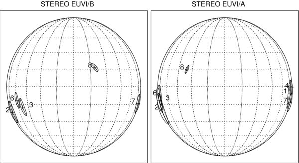
Figure 4. Location and and azimuthal extent of detected EUV dimming regions for STEREO EUVI/A (right panel) and EUVI/B (left panel). No dimming region was detected for event 1 by EUVI/B. The sizes of the EUV dimming regions are to scale. The positions are averaged over the three wavelengths. (The orientation of the coordinate system corresponds to the original EUVI/A and B images, but is close to the heliographic coordinate system.
Download figure:
Standard image High-resolution image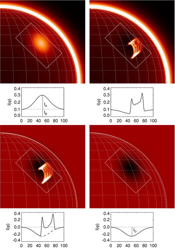
Figure 5. Numerical simulation of our method to determine the EUV dimming profile in azimuthal direction is shown. Top left: quiet Sun with stratified atmosphere and active region with enhanced density. Top right: the same portion of the corona after a CME was launched, leaving a dimming behind in the active region with growing postflare loops. Bottom left: difference image of the post-CME and pre-CME images shown in the top panels. Bottom right: theoretical difference image without flare loops. An image stripe is extracted in an azimuthal-radial coordinate system in each image, with the azimuthal profile (thick curve) shown in the inserts below each image. In order to separate the EUV dimming from the bright postflare loop EUV emission, a lower envelope is constructed, based on the dimmest data points in pre-CME subtracted difference images (dashed curve in bottom left panel). Note that this lower envelope matches the theoretical dimming profile without postflare loops (bottom right panel).
Download figure:
Standard image High-resolution image
with r0 being the radial distance of the centroid of an active region from the Sun center, as depicted in Figure 5 (top left panel and insert below). After the launch of a CME, a large fraction of the active region exhibits EUV dimming, but there occur also new postflare loops that are very bright in EUV (Figure 5, top right panel), which cannot easily be eliminated in difference images (Figure 5, bottom left panel). Our strategy is to reconstruct a lower envelope to the azimuthal flux profile of the difference image before (at time t1) and after (at time t2) the CME launch

Note that the background flux IB(r) drops out in the difference profile Idim(r, φ, t). We reconstruct a lower envelope in the azimuthal direction at the dimmest position in the difference images, in order to filter out the bright EUV emission of postflare loops, as the simulated example demonstrates (dashed curve in Figure 5 bottom left). The dimming profile Idim(φ, t2) at time t2 is reconstructed by fitting a Gaussian function through the dimmest point in a smoothed difference image Idim(r, φ, t2), which is a function that has only two free parameters (ID and σD at time t2),
as illustrated in Figure 5 (bottom right panel and insert below). We correct also for the spatial offset between the brightest pre-CME location and the dimmest post-CME position according to the two-dimensional (2D) brightness distribution I(r, φ) defined in Equation (10). We find that the full width of the EUV dimming region is nearly identical to the full width of the active region (i.e., σD ≈ σA) in cases without interfering postflare loops, and thus we can use it also as a robust measure of the width of the EUV dimming region, rather than fitting the ragged dimming profile Idim(φ) that is often contaminated by bright flare loops. Otherwise, the width σD of the dimming region would be significantly underestimated when bright postflare loops are present. This procedure efficiently filters out the contaminating EUV-bright flare and postflare loops, as long there exist still some dark locations in the dimming region that are not outshone by flare loops. A physical limit for the maximum dimming flux is the maximum pre-CME EUV brightness, i.e., ID ⩽ (IA + IB) (see also definitions of IA, IB, and ID in profiles shown in Figure 5).
An example of an EUV dimming measurement is shown in Figures 6 and 7. A time sequence of analyzed EUV difference images is shown in Figure 6, for event 2. The initial image of the pre-CME flux at 195 Å is shown in Figure 7 (top left panel), with the azimuthal flux profile of the active region fitted by a Gaussian (Equation (10)), yielding the flux values IA, IB, and width σA (second left panel). The final difference image (Equation (11)) is shown in Figure 7 (middle left panel), with the lower envelope fitted by a Gaussian function with the same width σD = σA (Figure 7, bottom left panel). The profile of the dimming flux at a central position of the dimming region is indicated with a hatched area (Figures 7–9), which also contains contamination (of the dimming flux) from bright postflare loop EUV emission. The evolution of the dimming flux is also shown for all 24 images separately (Figure 7, middle column), or as a function of time, Id(t) (Figure 7 top right). We see that the final dimming flux qD(t) = Id(t)/(IA + IB) approaches a value of qD ≈ 0.63, so the EUV brightness drops by more than half of the initial pre-CME brightness in the active region. The corresponding plots of the same event for both spacecraft and all wavelengths shown in Figure 8 exhibit little flare contamination for spacecraft EUVI/A 171 and 195 Å, for which the primary flare emission was occulted, but much stronger contamination for EUVI/B, for which the postflare loops were visible on the disk. In Figure 9, we show the corresponding plots for all other analyzed CME events (1, 3, 6, 7, and 8) in the same format as shown for event 2 in Figure 8, for the EUVI/A spacecraft and the 195 Å wavelength. A sensitive test of the robustness of our dimming reconstruction technique will be the comparison of obtained CME masses presented in the following.
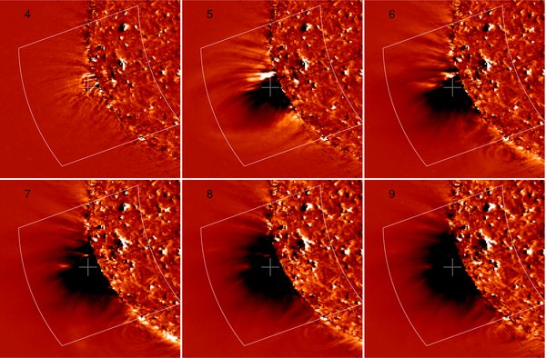
Figure 6. Sequence of 6 pre-CME subtracted difference images obtained by EUVI/A, 195 Å for event 2, covering the time interval of 2007 December 31, 00:00–04:00 UT, recorded with a cadence of 10 minute. The sequence shows the progressing EUVI dimming, clearly discernible after frame 2 (00:50 UT). A radial-azimuthal area is marked that has been extracted to derive the azimuthal EUV dimming profile I(φ) and angular width of the CME. The dimming analysis of this image set is shown in Figure 7.
Download figure:
Standard image High-resolution image
Figure 7. From the image sequence shown in Figure 6 (event 2, 2007 December 31, EUVI/A, 195 Å), the first CME image at 00:00 UT is shown in total EUV intensity (top left), with the corresponding azimuthal intensity profile I(φ) plotted below and fitted with a Gaussian function. The difference image of the last frame of Figure 6 at 03:50 UT shows the progressing dimming (middle left panel) along with the dimming profile Idim(φ) in the panel below, for which a lower envelope Gaussian shape is reconstructed. The middle panel shows Gaussian reconstructions of the dimming profiles Idim(φ) for all 24 images, of which are shown in Figure 6. The time evolution of the dimming amplitude Idim(t) (top right panel) is fitted with a Gaussian function. The CME mass (middle right panel) approaches an asymptotic value of m195 = 4 × 10¹⁵ g in the temperature range of the 195 Å filter.
Download figure:
Standard image High-resolution image
Figure 8. Pre-CME EUVI total flux images before flare start at 2007 December 31 (t1 = 00:00 UT), (event 2; top row) and difference images in the later EUV dimming phase (around t2 = 04:00 UT) (third row) for both spacecraft EUVI/A (left half) and EUVI/B (right half) in all three wavelengths 171, 195, and 284 Å are shown. The cross-sectional flux profiles I(φ, t1) (second row) and difference profiles I(φ, t2) − I(φ, t1) (bottom row) are shown (thin curves and hatched areas) at the positions marked with a solid or dashed line in the images. The pre-CME flux profiles are fitted with a Gaussian (thick curve in second row). The Gaussian curve that is overlaid on the difference profiles (bottom row) represents a slice of the 2D Gaussian fit to the lower envelope of the entire dimming region, suppressing the bright EUV emission from postflare loops.
Download figure:
Standard image High-resolution image
Figure 9. Pre-CME EUVI total flux images before CME launch (top row) and difference images late in the dimming phase (third row) for all other events (1,3,6,7,8) not shown in Figure 8 (event 2), observed from spacecraft EUVI/A at 195 Å. The representation is similar to Figure 8, with the pre-CME flux profiles (second row) and post-CME dimming profiles (bottom row).
Download figure:
Standard image High-resolution imageIn summary, we developed a robust algorithm that measures the EUV peak flux IA, coronal background IB, and geometric width σA of the pre-CME active region at time t1, as well as the EUV flux ID (with width σD ≈ σA) of the dimming region at times after the EUV dimming starts (when the CME takes off). The values of the fluxes IA, IB, ID, dimming ratios qD = ID/(IA + IB) ⩽ 1 are listed in Table 2 for each of the six detected events, both EUVI/A and B spacecraft, and all three wavelengths (171, 195, and 284 Å). These observables will be the basis for the calculation of the CME masses described in the next section.
2.5. Determination of Electron Density and CME Mass
We determine now the electron density ne and CME mass in the EUV dimming region, based on the observables of IA, IB, and ID, with the dimming region defined by the geometry of a 2D Gaussian function with Gaussian width σD (Figure 5). The FWHM of the Gaussian flux distribution is defined by  . In addition, since the EUV flux I(φ) is proportional to the squared electron density, i.e., I ∝ n2e (e.g., Equation (2)), the FWHM of the density distribution is another factor
  larger, so the relevant full width of the CME mass is

This yields the volume of the dimming region VD or the CME volume VCME before CME launch according to Equation (8). In order to obtain the CME mass mCME (Equation (7)), we need to determine the electron density ne in the active region that covers the EUV dimming volume VD.
The total EUV flux of an active region is composed of (1) the emission measure of the active region (with density nA) and (2) the emission measure of the coronal foreground and background along the same line of sight (with density nB). Usually the background density nB is measured from the background level outside of the active region and the background-subtracted excess flux IA of the active region is dependent on the background density nB as

where Δz is the column depth of the active region, Δx2 is the pixel area, and RT is the instrumental response function per pixel area.
For the determination of the average dimming mass in the same volume of the active region, we can now use the proportionality of the dimming flux (or the emission measure) to the square of the electron density, as it generally holds for optically thin EUV emission,
to obtain the mass loss md(t) associated with the EUV dimming. Note that the initial density associated with EUV dimming is zero before CME launch, i.e., nd(t = t0) = 0 and Id(t = t0) = 0, while the dimming-associated density nd(t = t2) = nD approaches the maximum value at the end of the dimming, when the dimming function approaches the value Id(t) = ID. The mass loss md(t) that makes up the CME mass can then be expressed as a function of time t and depends on the observables Id(t), IA, nA, and wD ≈ wA only
Note that this expression contains only the CME mass detected with a particular EUV filter (with temperature T), while the total CME mass needs to be synthesized from multiple temperature filters. The so-determined electron densities nA of the active region (pre-CME) volumes and dimming masses mD(t = t2, T) are listed in Table 2 for each event, spacecraft, and EUV filter temperature T ≈ 1.0, 1.5, 2.0 MK separately. The active region densities have a mean of nA = (5.0 ± 3.8) × 108 cm−3 (per filter) and are only slightly higher than the average densities of the coronal background, i.e., nB = (3.3 ± 0.6) × 108 cm−3. For the dimming masses, we find an average of mD ≈ (1.5 ± 1.1) × 1015 g per EUV filter (see averages at bottom of Table 2).
2.6. Temperature Synthesis of CME Masses
In Figure 10, we plot the dimming masses mD(t = t2, T) that have been detected at the end time (t = t2) of the analyzed time interval in each of the three EUV filters, which have the following FWHM temperature ranges: T171 = 0.51–1.25 MK for the 171 Å filter, T195 = 1.05–1.90 MK for the 195 Å filter, and T284 = 1.54–2.87 MK for the 284 Å filter. Since the three temperature ranges are slightly overlapping, we have to normalize the dimming masses by the temperature interval ΔT in each filter in order to obtain a differential emission measure-type mass distribution ΔmD(t, TF)/ΔTF. We fit then a Gaussian curve that has the same integrated mass in each filter temperature range and integrate the differential mass distribution to obtain the total mass of the dimming volume or CME

where T1 = 0.51 MK and T2 = 2.87 MK are the lower and upper bounds of all three EUVI filters combined together. Note that the peak temperature of the Gaussian fit is typically around T0 ≈ 1.5 MK, which proves that most of the CME mass is detected in the 195 Å filter, where also CME-associated EIT waves are best visible. The numerical values of the so-obtained CME masses mCME are listed in Figure 10 and in Table 3, for both EUVI/A and B spacecraft separately. The values from spacecraft A and B are consistent with an average ratio of mA/mB ≈ (1.3 ± 0.6).
Figure 10. Distributions of CME masses measured with EUVI/A (left panels) and B (right panels) for the five detected EUV dimming events. The mass dm/dT is scaled in units of dm = 1015 g per temperature interval dT = 1.0 MK, obtained separately for each of the three wavelength filters (171, 195, 284 Å), which have an overlapping response function (with the FWHM indicated with hatched boxes). They are fitted with a Gaussian function and integrated over the temperature interval of T = 0.5–3.0 MK, to obtain the full CME masses.
Download figure:
Standard image High-resolution imageTable 3. CME Masses and Widths Measured with EUVI and COR2 of Eight CME events
| Events | wA | wB | mEUVI/A | mEUVI/B | mEUVI | mCOR2,A | mCOR2,B | mCOR2 | mEUVI/mCOR2 |
|---|---|---|---|---|---|---|---|---|---|
| 1 | 225 | 167 | 2.3 | 5.5 | 3.9 | 2.23 | 2.57 | 2.57 | 1.51 |
| 2 | 254 | 203 | 6.1 | 6.9 | 6.5 | 7.10 | 7.68 | 7.70 | 0.84 |
| 3 | 214 | 169 | 6.4 | 3.5 | 4.9 | 5.29 | 3.59 | 5.29 | 0.93 |
| 6 | 196 | 172 | 5.7 | 2.9 | 4.3 | 2.86 | 1.27 | 2.87 | 1.49 |
| 7 | 153 | 168 | 3.7 | 2.3 | 3.0 | 2.84 | 1.89 | 2.84 | 1.05 |
| 8 | 142 | 148 | 2.3 | 2.5 | 2.4 | 2.78 | 0.94 | 2.80 | 0.85 |
Note. CME width from EUVI/A wA (deg), CME width from EUVI/B wB (deg), CME mass from EUVI/A mEUVI,A, CME mass from EUVI/B mEUVI,B, two-spacecraft constrained CME mass from EUVI mEUVI, CME mass from COR2/A mCOR2,A, CME mass from COR2/B mCOR2,B, two-spacecraft constrained CME mass from COR2 mCOR2 (all in units of 1015 g), CME mass ratio mEUVI/mCOR2.
Download table as: ASCIITypeset image
2.7. CME Mass Comparison from EUVI with COR2
In Figure 11, we compare our results of the CME masses measured from EUVI with those of COR2, given in Colaninno & Vourlidas (2009). The diamonds mark the improved CME masses derived from the mass ratio of COR2/A and B, while the horizontal bars indicate the mass difference measured between COR2/A and B. For the determination of CME masses with EUVI it is not clear a priori how the results from EUVI/A and B should be weighted. On one side, we expect that the less occulted spacecraft has a fuller view on the CME and thus sees the EUV dimming more completely, but on the other side slight occultation helps to block out the unwanted contaminating bright EUV emission from flare loops, which makes the reconstruction of the EUV dimming volume less contaminated and more reliable. We thus give equal weight to both spacecraft and average the CME masses measured by A and B, indicating the difference measured with A and B with the vertical error bars in Figure 11. The COR2 and EUVI measurements correlate well, with a mean and standard deviation of mEUVI/mCOR2 = 1.1 ± 0.3, so they agree typically within ±30%.

Figure 11. Comparison of CME masses measured with EUVI/A+B (y-axis) and COR2/A+B (x-axis). The diamonds mark the CME mass averaged from both EUVI/A+B spacecraft vs. the two-spacecraft constrained CME mass inferred from COR2 (corrected for the CME propagation angle to the line of sight). The error bars in either horizontal or vertical direction indicate the range between the measurements from spacecraft STEREO/A and B. The confusion limit of the EUV method is estimated to be ≲1.5 × 10¹⁵ g, below which CME detections on the disk are not reliable with our method.
Download figure:
Standard image High-resolution imageFor events 4 and 5, we detect no reliable EUV dimming, which could be because of either complete occultation or absence of dimming. The EUV dimming levels we measured for these two events are comparable with CME-unrelated dimmings, such as cooling of bright points or time variability of other small-scale sources. We also performed a null test by running our automated EUV dimming code at a random location near the solar north pole (where no CME is expected) and measured a residual mass equivalent of mres ≈ 0.6 × 10¹⁵ g (event 0 in Figure 11 bottom left). Thus, we consider this limit of ≲1015 g as an empirical confusion limit for CME detection on the disk with our automated code. Above the limb, where chromospheric EUV emission is absent, our method can detect much fainter dimming levels.
The differences in CME masses determined from EUVI/A and B can arise from a number of model assumptions, such as the cylindrical 3D geometry, the circular footpoint area, the hydrostatic scale height, the temperature derivation from the peak of the EUV response function, but also from perspective effects from different spacecraft viewing angles, such as different degrees of occultation of dimming regions as well as postflare loops. While it is difficult (and probably unreliable) to quantify uncertainties for each model parameter formally, the obtained difference in the final result of CME masses between EUVI/A and B provides a reliable (empirical) error for a single-spacecraft measurement, which constitutes a smaller absolute error for the combined two-spacecraft measurement.
2.8. Time Evolution of CME Dimming and Coronal Mass Loss
We show the time evolution of the EUV dimming 1 − Id(t)/(IA + IB) in Figure 12, normalized by maximum pre-CME flux (IA + IB). In order to characterize the dimming time, we fit a semi-Gaussian curve to the time evolution, with ID representing the maximum dimming flux ID = Id(t ≫ t0),
which yields an objective measure of the dimming starting time t0 (within the definitions of our model), the EUV dimming timescale tD (when the dimming flux drops from unity to the level of exp(−1) ≈ 0.61), and the final dimming level ID. The statistics of all dimming times yield a mean and standard deviation of tD = 1.3 ± 1.4 hr (see bottom of Table 2). The dimming starting times often agree for both spacecraft within a fraction of the dimming time tD.
The average dimming level at the end of the analyzed time interval is qD = 1 − I(t2)/(IA + IB) = 0.47 ± 0.37, so the brightness dropped to a factor of ≈1/2, which corresponds to a density drop of  (Equation (15)). We have to be aware, however, that this refers to the pre-CME brightness level of the active region. Since the pre-CME EUV emission of an active region has an average excess brightness of IA ≈ 200 ± 210 DN s−1, which is comparable with the average background level IB ≈ 170 ± 160 DN s−1 (see bottom of Table 2), a dimming fraction of 50% in ID/(IA + IB) essentially eliminates all the excess emission of an active region. This is particularly true for limb events, which are most of the events (except event 8). This is a surprising new fact that has not been appreciated or quantitatively measured before. In other words, virtually all plasmas in an active region are evacuated away from the Sun, except for new flare loops that are created after the launch of the CME and gradually fill in the new vacuum. Consequently, we would expect completely dark dimming regions for a CME launch at the disk center, if the CME evacuation channel is aligned with the line of sight. However, inspecting Figures 12 and 2, we find no clear trend whether the final dimming level or dimming time depends on the viewing angle (different spacecraft), wavelength, or location (different events).
Figure 12. Time evolution of the EUV dimming observed for the five major events (2,3,6,7,8 in different rows), for all three wavelengths (171, 195, and 284 Å in different columns), for both spacecraft EUVI/A (black) and B (gray color). The EUV dimming flux 1 − Id(t)/(IA + IB) is normalized to the pre-dimming level at time t = t1. The EUV dimming fluxes measured in each time frame are displayed as a histogram (with the bin width corresponding to the EUVI cadence) and a semi-Gaussian curve is fitted to characterize the EUV dimming starting time t0 and e-folding dimming time tD (smooth curve).
Download figure:
Standard image High-resolution imageThe CME mass md(t) scales proportionally to the dimming-associated density (Equation (16)), which allows us to quantify the time evolution of the mass loss md(t) as a function of time. We show this observed mass loss evolution in Figure 13 for the major five events from spacecraft EUVI/A, 171 Å (which has the highest cadence), scaled to the total mass loss detected in all EUV filters). According to the semi-Gaussian fit of the dimming function Id(t) (Equation (18)) and the mass–density relationship (Equation (16)), we can express the mass loss with the analytical approximation,
The slopes of the mass loss function dmd(t)/dt (see Figure 13) vary more than an order of magnitude between different CMEs. The CME with the fastest mass loss is associated with the largest flare (6, GOES M1.7 class, 2008 March 25), but the mass loss rate does not correlate with the flare magnitude for the other events.
Figure 13. Time evolution of CME mass loss for the five well-detected events (2,3,6,7,8). The datapoints (histograms) are taken from the EUVI/A 171 Å filter, scaled to the total CME mass of all synthesized filters together and averaged from both spacecraft. The smooth curves are derived from the semi-Gaussian fits to the EUV dimming curves (Figure 12). Note that the biggest flare (event 6, GOES class M1.7) has the fastest mass loss rate, but not the biggest final mass (event 2, GOES class B1.5).
Download figure:
Standard image High-resolution image2.9. Time Evolution of CME Expansion
The time evolution of the dimming mass md(t) is monotonically increasing as more CME mass leaves the corona. This is the consequence of the adiabatic expansion of the CME bubble, which is a dynamically expanding magnetic field structure that confines the enclosed plasma. We can therefore relate the density evolution n(t) = n0 − nd(t) in the expanding volume VD(T) (of the dimming region) to the pre-CME density n0 and volume V0 according to mass conservation inside the CME bubble,

which implies a reciprocal relationship between density and volume. For the geometry of the CME bubble, we might use a 3D shape that expands in a self-similar way, so that the volume scales with the third power of its vertical extent h(t), which can be the geometry of a spherical bubble, an ice cone, or a flux rope,
The self-similar expansion yields the following time evolution for the expanding height h(t) (using Equations (20) and (21)):
Since the electron density scales with the square root of the intensity for optically thin EUV emission (Equation (15)), we expect the following evolution as a function of time (using the approximation of Equation (18)),
From this model, we can also characterize the CME front speed v(t):
Based on the expression of Equation (23), we can predict the time delay ΔtCOR2 between the CME arrival at COR2 and the CME launch time t0 at EUVI,
where the radial distance is hCOR2 ≈ 4 solar radii (for a launch site near the disk center, or hCOR2 ≈ 3 solar radii for a launch near the limb), and the initial height is the mean height in a gravitationally stratified atmosphere, i.e., a thermal scale height, h0 ≈ λT.
The measured dimming times tD are listed for each event, spacecraft, and wavelength in Table 2. Inspecting the values of tD and the fitted curves in Figure 12, we notice some discrepancies between the values obtained from different spacecraft, which ideally should be similar. There are several reasons for inconsistencies that affect the results differently for the two spacecraft views: (1) bright EUV emission from postflare loops can significantly hamper the reconstruction of the EUV dimming curve, which tends to lead to overestimates of the dimming time; (2) occulted emission underestimates the dimming mass; or (3) vertical gradients in the CME mass loss leads to stronger dimming for hotter plasma (with larger density scale heights), etc. These effects need to be investigated in more detail and will be pursued in a future study. At present, we recommend to use the shortest dimming time among the values determined from different views (spacecraft) and wavelengths for each event.
As an example, we test event 6, the CME event of 2008 March 25, 18:40 UT, which shows a well-defined self-similar expansion of a spherical bubble and has been analyzed in various studies (e.g., Aschwanden 2009; Zhang 2008). From our semi-Gaussian fits to the EUV dimming profiles, we found dimming times of tD = 0.11 hr for EUVI/A 195 Å (discarding the shorter dimming time of tD = 0.05 hr obtained in 171 Å because of partial occultation for EUVI/A), and the same value tD = 0.11 hr for EUVI/B 171 Å (which is the shortest among the different wavelengths). Using this dimming time values and the exponential height-time model (Equation (23)), we predict time delays of Δt = 0.70 ± 0.02 hr (after a start time of 18:38 UT in EUVI/A and 18:27 UT in EUVI/B) for the arrival at COR2 after a travel distance of 3 solar radii (Figure 14). COR2 reports an earliest detection of the CME in both COR2/A+B at 19:22 UT, which corresponds to a delay of Δt = 0.82 ± 0.09 hr, which is consistent within ≈10%. Alternatively, the self-similar expansion of the CME bubble was measured by fitting a spherical geometry to the periphery of the CME bubble and fitted with a quadratic height dependence (Aschwanden 2009),

with best-fit values of h0 ≈ 40 Mm, v0 ≈ 0, and a ≈ 0.4 km s−1. We plot this height-time fit in Figure 14 also, which yields a prediction of a time delay of Δt = 0.89 hr at COR2, which is also consistent with the COR2 detection time within ≈10%. Comparing the two methods, we notice a different functional dependence, which implies that the approximations must break down at some distance. The EUV dimming could only be constrained in the lowest altitudes in the corona, while the spherical expansion can be detected out to the edge of the EUV field of view (1.6 solar radii) and further (using the lateral expansion). We envision therefore that a combined measurement method for the EUV dimming and CME expansion could lead to a more self-consistent model and provides the missing link between the CME origin in the lower corona and CME propagation in the heliosphere as observed by coronagraphs (which have to block out the lower corona with an occulting disk).
Figure 14. Height-time plot of CME event 6 (2008 March 15, 18:40 UT): From the EUVI dimming curves at times of t − t0 ≲ 0.2 hr and extrapolating the exponential height dependence h(t) (Equation (23)), we predict delays of Δt = 0.68 hr (EUVI/A 195 Å) and Δt = 0.72 hr (EUVI/B/171 Å) for the arrival time in the COR2 field of view at h = 4 solar radii (thin curves and diamond symbols), while COR2 reports detection of the CME in both COR2/A and B after a delay of Δt = 0.8 hr after the beginning of the EUV dimming at 18:40 UT. The fitting of the self-similar expansion of the CME bubble with a circular shape and fitted with a quadratic height-time function in the range of Δt ≲ 0.7 hr (Aschwanden 2009) predicts an arrival time delay of Δt = 0.89 hr.
Download figure:
Standard image High-resolution image
3. DISCUSSION
3.1. EUV versus White-Light Observations of CMEs
This is one of the first systematic studies that quantitatively compares CME observations in EUV and white light. There are a number of fundamental differences between the two wavelengths. First, white-light observations record photospheric photons that get scattered in the corona and heliosphere (i.e., Thomson scattering), and thus is sensitive to all electrons independent of their temperature. Emission in EUV wavelengths, in contrast, is mostly produced by thermal bremsstrahlung (free–free emission) of energized electrons with ambient ions, as well as by line emission from free-bound transitions, excitations, and ionizations of atoms. Since EUV filters have a narrow-band response function, each filter is sensitive to a particular temperature range. For the three coronal EUV filters of STEREO/EUVI, this temperature range is approximately T ≈ 0.5–2.9 MK, which covers the bulk (i.e., the peak of the distribution) of the coronal mass in active regions, the quiet Sun, and coronal holes, and thus we expect that they also catch the bulk of the low coronal component of CME masses. Therefore, this comparison of CME masses derived from EUV versus white light represents an important test whether this assumption is true. We find indeed a very good correspondence between the two methods here, with a ratio of mEUVI/mCOR2 = 1.1 ± 0.3, which corroborates the self-consistency of both methods. It is conceivable that we do not recover identical masses with both methods, if for instance CMEs contain a significant fraction of cold chromospheric mass (i.e., prominences), or if some CME mass that gets expelled from the lower corona would fall back at altitudes r < 4 solar radii before it is detected with COR2. Such coronal inflows in the trailing wakes of CMEs were indeed detected before (e.g., Wang et al. 1999; Sheeley & Wang 2002), but apparently they do not carry a significant mass fraction of the CME.
The limited temperature range of EUV filters apparently does not truncate the measured CME masses, although we are only sensitive in the temperature range of T ≈ 0.5–2.9 MK. Our three-point CME mass distribution (Figure 10) indeed suggests that the peak of the CME mass distribution occurs around T ≈ 1.5 MK, which renders the 195 Å wavelength filter to the most important sensor of CME masses. It was already noticed before that EIT waves, which are a side product of CMEs, were seen with the best contrast in the 195 Å filter (e.g., Wills-Davey & Thompson 1999; Delannee 2000). Our analysis adds the same preference for the 195 Å filter in observing and detecting EUV dimming and associated CMEs.
Interesting consequences arise also from the non-cospatiality of the detection of EUV dimming and associated CMEs in the lower corona (≲0.1 solar radius) and the white-light coronagraph detection with COR2 (at ⩾4 solar radii). Since we expect that most of the CME mass should propagate outward, and therefore will show up after some time in the coronagraphs, we should expect that every EUV dimming event should lead to a CME detection with COR2, unless they fall below the sensitivity threshold. Currently, we find a lower mass limit of mCME ≈ 1.0 × 10¹⁵ g from the detection of EUV dimming, while detections of lower values appear to be related to cooling bright points or cooling loop structures, rather than leaving CMEs. Vice versa, we do not expect a dimming signal in EUV for every COR2 detection of a CME, because some of the CMEs may originate high in the corona where the EUV intensity is very low or they might originate on the backside of the Sun, where EUV emission is obscured or occulted (near the limb), unless the STEREO spacecraft cover some fraction of the Sun's backside. For our observation period, the two STEREO spacecraft cover already approximately a quarter of the Sun's backside, and thus we expect an EUVI detection rate of five out of eight, as indeed observed. Although the COR2 observations suggest that all eight selected CMEs originate on the frontside of the Sun or near the limb, four cases are partially occulted for at least one of the spacecraft, while one of the localization is dubious, suggesting a high altitude origin for the CME. In any case, the complementarity of EUVI and COR2 observations provides important information on the source region of CMEs.
3.2. Previous CME Mass Determinations from EUV Dimming
The first measurements of the CME masses using EUV observations of coronal dimmings were reported by Harrison & Lyons (2000). A small CME observed with LASCO in white light with a mass of mCME = (5 ± 1) × 1013 g was spectroscopically observed with SOHO/CDS also. The authors determined from the Si X 356 Å/347 Å ratio a density of ne = 109 cm−3 in the center of the dimming region. From a rough estimate of the projected dimming area in Mg IX 368 Å, the authors arrive at a mass estimate of mCME = 3.3 × 10¹³ g, which amounts to 70% of the white-light estimate. Comparing with our method presented here, the EUV-based mass estimate could further be improved by quantifying the unprojected CME footpoint area and the vertical density scale height to obtain a more accurate estimate of the 3D dimming volume (Equation (8)), as well as modeling of the fore/background density along a line of sight (Equation (5)) in order to obtain an uncontaminated density in the dimming region.
In a follow-up study by Harrison et al. (2003), a total of five CME events were analyzed based on LASCO and SOHO/CDS observations, including the event analyzed in Harrison & Lyons (2000). The CME was determined from the EUV dimming within a box that encompasses the darkest dimming area, using two different methods to extrapolate the mass loss over a comprehensive temperature range: (a) using a canonical DEM curve for active regions specified in Raymond & Doyle (1981), and (b) the density derived from the Si X 356 Å/347 Å line ratio. The CME masses derived from white light and EUV have ratios of mCME/mEUV = 1.2, 0.3, 4.7, 0.01, 0.7 with the DEM method, and mCME/mEUV = 0.4, 0.07, 1.0, 0.004, 0.3 with the line-ratio method. The biggest discrepancy was found for the fourth event, where we suspect that the dimming volume was largely overestimated according to the box chosen in their Figure 7. If the box is overestimated by a factor of L = 2, the resulting volume and CME mass would be overestimated by a factor of V ≈ L3 = 8. Also the contamination from postflare loops, which causes bright EUV emission in the EUV dimming region, may enter large uncertainties in electron densities derived from line ratios averaged over a box that contains both dimming and flare loop emission. Three-dimensional volume modeling of the EUV dimming region and elimination of flare loops are thus essential for improving the accuracy of CME mass estimates based on EUV dimming. In our study, we modeled these effects in detail and arrived at much smaller differences between white light and EUV masses, i.e., mCOR2/mEUVI = 1.1 ± 0.3. In addition, we benefit from the redundancy of dual stereoscopic imaging observations here, while the observations of Harrison et al. (2003) were based on a spectroscopic single-spacecraft instrument.
A CME mass based on EUV dimming was also derived in Zhukov & Auchere (2004), who got a fair agreement with the white-light CME mass. The authors measure the area A of the dimming region and assume a volume of V = AλT extending over a thermal scale height, similar to our method (Equation (8)). The authors perform some DEM modeling based on three EIT filters (similar to our method), but the three-filter EIT data set was taken three hours before the CME event, while all our three-filter EUVI data sets are strictly simultaneous with the CME and dimming events (thanks to the higher cadence of multi-filter observations of STEREO/EUVI).
3.3. The Relationship between EUV Dimming and CMEs
Throughout this paper, we made the tacit assumption that a detected EUV dimming is identical to the coronal mass loss of a CME, and vice versa we expect that every detected CME should also cause an EUV dimming, unless the CME originates in the upper corona (where we have little EUV emission because of the gravitational stratification). The latter case, however, would imply very low masses compared with a CME that originates at the base of the corona, i.e., ≈30% at one thermal scale height, or ≈10% at two thermal scale heights. In fact, the detection probability should equally drop for both EUV and white-light coronagraphs with altitude, because the detection threshold scales with the total mass of CMEs in both cases.
A number of studies of coronal dimming as a means for identifying CME source regions have been undertaken, focusing on transient coronal holes caused by filament eruptions (Rust 1983; Watanabe et al. 1992), EUV dimming at CME onsets (Harrison 1997; Aschwanden et al. 1999), soft X-ray dimming after CMEs (Sterling & Hudson 1997), soft X-ray dimming after a prominence eruption (Gopalswamy & Hanaoka 1998), or simultaneous dimming in soft X-rays and EUV during CME launches (Zarro et al. 1999; Harrison & Lyons 2000; Harrison et al. 2003). All these studies support the conclusion that dimmings in the corona (either detected in EUV, soft X-rays, or both) are unmistakable signatures of CME launches, and thus can be used vice versa to identify both phenomena. A statistical study on the simultaneous detection of EUV dimmings and CMEs has recently been performed by Bewsher et al. (2008). This study based on SOHO/CDS and LASCO data confirms a 55% association rate of dimming events with CMEs, and vice versa a 84% association rate of CMEs with dimming events. Some of the non-associated events may be caused by occultation, CME detection sensitivity, or incomplete temperature coverage in EUV and soft X-rays. Their detection rate is consistent with ours, since we detect EUV dimming in six out of the eight cases (75%). Perhaps this CME-dimming association rate will climb up to 100% once the STEREO spacecraft reaches a separation of 180° and cover all equatorial latitudes of the Sun.
4. CONCLUSIONS
In this study, we model CME masses from EUV observations and validate the results by comparisons with CME masses determined from white light observations. There exist some previous studies with estimates of CME masses based on EUV dimming with simple treatments of the dimming area and average density, while our method includes 3D modeling of the volume and density in the dimming region and ambient corona. Our code contains the following tasks: (1) measuring the coronal background density in the foreground and background of an EUV dimming region along any arbitrary line of sight, (2) modeling the 3D volume of the EUV dimming region in terms of a cylindrical geometry, (3) modeling the average density inside the dimming volume for any given aspect angle and as a function of time, (4) calculating the volumetric mass deficit of the dimming region, and (5) synthesizing the mass deficits from different temperature filters to estimate the total CME mass. As a test, we compared then the CME masses obtained from STEREO/EUVI A+B observations with those from STEREO/COR2 A+B and find an agreement within a factor of mEUVI/mCOR2 = 1.1 ± 0.3. The time-dependent measurement of the EUV dimming curve over several hours allows us also to model the evolution of the CME volume in terms of adiabatic expansion of a self-similar geometric shape, which provides a direct prediction of the height-time and expansion velocity of a CME. We test one case by comparing the predicted arrival times at COR2 with the actual detection times reported by COR2 and find agreement within ≈10%. However, further studies are required to bring the dimming times measured in different wavelengths and with different spacecraft into satisfactory agreement for other cases. In summary, this study demonstrates the complementarity of EUV and white-light observations in the detection, tracking, and modeling of CMEs, where EUV provides detailed information on the source region that is occulted for white-light coronagraphs. In principle, the same technique can be applied to single-spacecraft observations in EUV, such as obtained with SOHO/EIT and TRACE, but the availability of dual spacecraft by STEREO provides the additional benefit of extended solar coverage, redundancy in background density models, and 3D capabilities to triangulate the true CME source position, propagation, and mass.
We thank the anonymous referee for very constructive comments that helped to improve the manuscript. This work is supported by the NASA STEREO under NRL contract N00173-02-C-2035. The STEREO/SECCHI data used here are produced by an international consortium of the Naval Research Laboratory (USA), Lockheed Martin Solar and Astrophysics Lab (USA), NASA Goddard Space Flight Center (USA), Rutherford Appleton Laboratory (UK), University of Birmingham (UK), Max-Planck-Institut für Sonnensystemforschung (Germany), Centre Spatiale de Liège (Belgium), Institut d'Optique Théorique et Applique (France), and Institute d'Astrophysique Spatiale (France). The USA institutions were funded by NASA; the UK institutions by the Science & Technology Facility Council; the German institutions by Deutsches Zentrum für Luft- und Raumfahrt e.V. (DLR); the Belgian institutions by Belgian Science Policy Office; the French institutions by Centre National d'Etudes Spatiales (CNES), and the Centre National de la Recherche Scientifique (CNRS). The NRL effort was also supported by the USAF Space Test Program and the Office of Naval Research.