


ABSTRACT
By fitting the Hipparcos Intermediate Astrometric Data (HIAD), photocentric orbits can be obtained for the single-lined spectroscopic binaries (SB1s). In previous work, a simplifying approximation used in the fitting process was that the photocenter coincides with the primary, but simple arguments based on a mass–luminosity relation show that this approximation will introduce non-negligible deviation into photocentric orbits of a few SB1s. By fitting the revised HIAD without the approximation, the present paper tries to provide reliable photocentric orbits for those SB1s in the 9th Catalogue of Orbits of Spectroscopic Binaries having a reliable spectroscopic orbit of period between 50 days and 3.2 years. After a stringent assessment and screening process, we finally accept the photocentric orbits of 72 systems. Among these results, 37 orbits are obtained here for the first time. So far, only three of these systems are resolved with a known relative orbit. For each of them, the paired photocentric and relative orbits are in reasonably good agreement. For the 25 systems with a main-sequence primary, the masses of component stars and the semimajor axes of relative orbits are estimated for the purpose of planning ground-based observations.
Export citation and abstract BibTeX RIS
1. INTRODUCTION
For about 106 spectroscopic binaries (SBs), the radial velocity curves of components and the astrometric wobbles of photocenters will be obtained, respectively, by two devices on board Gaia, i.e., the Radial Velocity Spectrometer and the Astrometric Instrument. In order to make the best use of these two types of observations, it will be necessary to develop an efficient method of fitting them simultaneously to the binary model.
However, when the radial velocity observation carries much more weight than the photocenter position observation, it is preferable to use the efficient two-step procedure (Jancart et al. 2005; Pourbaix & Boffin 2003): As the first step, spectroscopic orbital elements are determined by fitting the radial velocity observations. Then, those photocentric orbital parameters that remain undetermined are determined by fitting the astrometric wobbles of the photocentric observation.
For those single-lined spectroscopic binaries (SB1s), a helpful assumption proposed by Jancart et al. (2005) is that the photocenter coincides with the primary, ignoring the light coming from the secondary. This means in particular that
where a0 and a1 are the angular semimajor axes of the photocentric and the primary orbits, respectively, and, ϖ, K1, P, e, and i are the system parallax, the semi-amplitude of the radial velocity curve of the primary, the orbital period, the orbital eccentricity, and the inclination, respectively. By fitting the Hipparcos Intermediate Astrometric Data (HIAD; ESA 1997; van Leeuwen 1998) with the approximation (Equation (1)), Jancart et al. (2005) obtain the photocentric orbits of 70 SB1s in the 9th Catalogue of Orbits of Spectroscopic Binaries ( ; available at http://sb9.astro.ulb.ac.be; Pourbaix et al. 2004).
In the case when the signal-to-noise ratio of astrometric data reaches a value comparable to the relative difference between a0 and a1, i.e.,  , this approximation is helpful to avoid unreasonable orbital solutions violating the necessary condition a0 < a1. However, when determining photocentric orbits with very accurate astrometric data such as those from Gaia, it will introduce non-negligible error into solutions of a certain type of SB1.
Given a stellar mass–luminosity relation (MLR), it is possible to estimate a priori the relative error of a0, i.e., δ, directly caused by using a0 = a1. To do so for binaries composed of main-sequence components, we resort to the MLR (Arenou et al. 2000)

where M (in solar mass) and Hp are the mass and the absolute Hipparcos magnitude of a star, respectively. From Equation (2), it is easy to deduce that
where ΔHp ⩾ 0 is the Hipparcos magnitude difference between the two components. The function δ(ΔHp) is plotted in Figure 1. From this figure, we see, for example, that δ increases with decreasing ΔHp and δ = 20% at ΔHp ∼ 2.9. In fact, this situation is relatively rare for most SB1s, which usually have a relatively large magnitude difference between the two components.
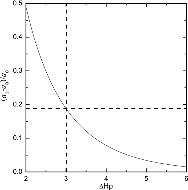
Figure 1. Relation between the Hipparcos magnitude difference ΔHp and (a1 − a0)/a0 for the SB1s composed by two main-sequence stars.
Download figure:
Standard image High-resolution imageOn the other hand, the HIAD have been revised and the precision of the revised HIAD total weight is improved with respect to its original version by a factor of 2.2 (van Leeuwen 2007a, 2007b). By virtue of this improvement, a few brown dwarf and planet secondaries have been found in SB1s (e.g., Kurster et al. 2008; Reffert & Quirrenbach 2011; Sahlmann et al. 2011a, 2011b; Sozzetti & Desidera 2010; Stefanik et al. 2011). Therefore, it is possible that new or improved photocentric orbits of SB1s might be obtained by fitting the revised HIAD.
A sample of 341 SB1s is selected from  in Section 2 and their photocentric orbits are determined and assessed by several screening criteria in Section 3. In Section 4, some interesting topics regarding SB1s are discussed based on reliable orbital solutions. Concluding remarks are made in Section 5.
2. THE SAMPLE OF SB1s
In  , there are about 1200 SB1s with a Hipparcos entry. A reliable photocentric orbit is expected only for some of them. The first limitation comes from the fact that only some of the SB1s in
  have a reliable orbit. For this, we restrict ourselves to those with an orbit grade larger than 3.0, and for the cases without such a grade, those with max (σe, σP/P, σT/P, σω/2π) ⩽ 0.01, where σ denotes the standard errors, with T and ω being the epoch of a periastron passage and the periastron argument, respectively. The second limitation is imposed by the observing frequency and the time span of HIAD. Taking this into consideration, we restrict ourselves further to SB1s with orbital periods in the range from 50 days to 3.2 yr (Casertano et al. 2008; Jancart et al. 2005). This screening process leaves us with a sample of 341 SB1s. To save space, the Hipparcos identifications of these SB1s are not listed here, and only those sample SB1s with reliable photocentric orbits obtained in the present paper will be listed in Section 3 after orbit assessment.
Among those 70 SB1s, the orbits of which have already been obtained in Jancart et al. (2005), 20 are not included in our sample due to the following facts. HIP 677, 7078, 8903, 87895, 89937, and 111170 have been resolved by the spectroscopic technique and are now double-lined. HIP 3504, 40326, 67480, 95575, and 101093 have orbital grades of less than 3.0. HIP 10514, 52085, 60998, 65417, 74087, 80346, 80686, 88788, and 109176 have orbital periods that are not in the range from 50 days to 3.2 yr.
3. PHOTOCENTRIC ORBIT DETERMINATION
Distributed along with the revised Hipparcos catalog, the HIAD as stored in the folder named resrec provides the abscissa residuals for each point source with respect to the final catalog solution, which often involves acceleration terms for an SB photocenter (van Leeuwen 2007a). For the details of how to use these data in the context of binary orbital determination, the reader is referred to Reffert & Quirrenbach (2011) and Sahlmann et al. (2011b).
A photocenter orbital determination method has been implemented in Jancart et al. (2005). When using this method, two types of solutions are obtained, i.e., the Campbell solution (SC) with parameters {e, P, T, ω, a0, i, Ω} and the Thiele-Innes solution (STI) with parameters {e, P, T, A, B, F, G}, where Ω is the ascending node and
Fitting the revised HIAD to give SC, we consider a0 as an adjusted parameter with the restriction a0 < a1, where a1 is calculated from expression (1), and the linear parameter ψ = cos i is used instead of the nonlinear i. To cope with the remaining single nonlinear parameter (Ω), a modified grid method (Ren & Fu 2010) is used to search for the global optimization solution.
Before applying various statistical tests, orbital solutions with i = 0° mod(180°) are rejected because they imply that the primary's radial velocity is constant, contrary to the spectroscopic observations (Jancart et al. 2005; Pourbaix & Boffin 2003). The remaining solutions are checked by all the tests detailed in Jancart et al. (2005) and Goldin & Makarov (2006). The consistency between SC and STI is indicated by α1 (Pourbaix & Boffin 2003; Ren & Fu 2010), the detective possibility of orbital wobble of the HIAD is indicated by α2 when using the F-test (Pourbaix & Jorissen 2000) and by α3 when using the Monte Carlo test (Goldin & Makarov 2006), the compatibility between the revised HIAD and the spectroscopic data is indicated by α4 (Jancart et al. 2005), and the correlation among the derived parameters is indicated by  (Eichhorn 1989; Jancart et al. 2005).
Following previous papers, we accept a solution with the screening criterion that α1, α2, α3, and α4 < 5% and > 0.4 are satisfied simultaneously, which ensures that the solution is reliable with a probability larger than 95%. The number of accepted solutions is 72. For these solutions, spectroscopic orbital parameters, apparent visual magnitudes, spectral types, and the relevant references are given in Table 1. The obtained photocentric orbital parameters, together with the values of the statistical indicators and the estimated semimajor axes of the primary orbits are given in Table 2.
Table 1. Spectroscopic Orbital Information (P, T, e, ω, K1), Apparent Visual Magnitudes mV, the Spectral Types and the Relevant References of the 72 SB1s with Reliable Photocentric Orbits
| HIP | P | T | e | ω | K1 | mV | Spectral | Reference |
|---|---|---|---|---|---|---|---|---|
| Identifier | Days | (JD-2,400,000.0) | (deg) | (km s−1) | Type | |||
| 705 | 71.550 | 46405.920 | 0.221 | 140.8 | 13.55 | 8.370 | G2V | Latham et al. (2002) |
| 2170 | 936.000 | 42531.900 | 0.000 | 0.0 | 12.60 | 8.200 | K1III | Griffin (1979b) |
| 5881 | 701.420 | 51791.100 | 0.120 | 313.0 | 3.02 | 8.850 | G5V | Nidever et al. (2002) |
| 5952 | 274.560 | 46253.000 | 0.337 | 103.0 | 6.74 | 8.460 | G5V | Latham et al. (2002) |
| 6306 | 847.700 | 47758.900 | 0.806 | 328.5 | 7.11 | 7.620 | F5V | Latham et al. (2002) |
| 7134 | 53.504 | 39810.880 | 0.390 | 278.1 | 24.30 | 7.810 | G5 | Griffin (1975) |
| 10340 | 748.200 | 37886.000 | 0.340 | 358.0 | 4.88 | 4.844 | K4III | Griffin & Herbig (1981) |
| 12062 | 905.000 | 46440.000 | 0.260 | 254.6 | 6.77 | 8.950 | G5V | Latham et al. (2002) |
| 17932 | 962.800 | 42288.100 | 0.720 | 108.8 | 20.20 | 5.668 | G2III | Pedoussaut et al. (1987) |
| 20982 | 699.300 | 45469.400 | 0.125 | 134.5 | 4.45 | 5.477 | G8III | Prieur et al. (2006) |
| 21433 | 332.500 | 47121.000 | 0.642 | 124.8 | 7.63 | 8.330 | K2V | Tokovinin et al. (1994) |
| 22607 | 143.530 | 44248.396 | 0.610 | 205.9 | 18.00 | 6.250 | F5V | Turner et al. (1986) |
| 23221 | 903.000 | 50384.000 | 0.300 | 171.0 | 4.80 | 5.399 | K0IV | Vennes et al. (1998) |
| 24331 | 1031.400 | 26182.460 | 0.100 | 17.9 | 8.70 | 4.481 | K0.5III | Bertiau (1957) |
| 24419 | 803.510 | 50690.000 | 0.080 | 275.0 | 3.59 | 7.450 | G7V | Nidever et al. (2002) |
| 26001 | 180.875 | 23108.418 | 0.510 | 330.0 | 22.40 | 5.349 | G9III | Lunt (1924) |
| 28814 | 1091.800 | 51788.000 | 0.246 | 223.1 | 11.90 | 5.635 | G4III | Griffin (2006) |
| 30338 | 628.889 | 48464.300 | 0.025 | 227.0 | 9.04 | 7.250 | K3IIIBa5 | Udry et al. (1998) |
| 31359 | 125.594 | 51933.900 | 0.046 | 95.0 | 16.84 | 6.460 | K0III | Griffin (2002b) |
| 32397 | 53.774 | 45253.710 | 0.000 | 0.0 | 93.40 | 7.220 | B5Ib | Mayer et al. (2001) |
| 33982 | 85.182 | 47518.430 | 0.237 | 20.8 | 22.67 | 9.450 | G0 | Latham et al. (2002) |
| 34164 | 612.300 | 47859.900 | 0.273 | 248.9 | 11.35 | 8.488 | G0 | Latham et al. (2002) |
| 39893 | 733.500 | 48342.000 | 0.212 | 210.0 | 4.05 | 9.650 | G3V | Latham et al. (2002) |
| 40772 | 89.065 | 42573.790 | 0.190 | 185.1 | 22.70 | 5.734 | G8III | Carquillat et al. (1983) |
| 45075 | 1062.400 | 25721.600 | 0.480 | 349.4 | 3.90 | 4.648 | Am | Bretz (1961) |
| 46893 | 830.400 | 43119.500 | 0.150 | 261.0 | 5.70 | 6.256 | K0 | Griffin (1981b) |
| 47461 | 635.400 | 45464.500 | 0.149 | 135.4 | 9.37 | 7.540 | F2 | Ginestet et al. (1991) |
| 50801 | 230.089 | 25577.030 | 0.060 | 236.4 | 7.40 | 3.066 | M0III | Jackson et al. (1957) |
| 50966 | 190.529 | 48063.800 | 0.248 | 124.4 | 9.45 | 8.120 | F5V | Torres et al. (1997) |
| 51157 | 1180.600 | 44583.000 | 0.869 | 296.1 | 7.99 | 8.240 | K1V | Griffin (1987) |
| 55022 | 663.180 | 46644.000 | 0.046 | 172.0 | 8.05 | 9.170 | F5V | Carney et al. (2001) |
| 57791 | 490.765 | 51667.700 | 0.271 | 126.4 | 13.60 | 5.635 | K0III | Imbert & Carquillat (2005) |
| 59468 | 461.000 | 22360.790 | 0.170 | 235.3 | 14.30 | 5.620 | K4III | Harper (1930) |
| 59750 | 843.900 | 47589.000 | 0.046 | 199.0 | 7.93 | 6.110 | F9V | Carney et al. (2001) |
| 61724 | 972.400 | 43304.000 | 0.590 | 102.5 | 10.50 | 5.490 | G9III | Griffin (1981a) |
| 62915 | 1027.000 | 43424.500 | 0.320 | 194.0 | 2.60 | 6.446 | K0 | Griffin (1983) |
| 63063 | 1042.600 | 45945.200 | 0.422 | 342.0 | 6.79 | 9.960 | K0V | Latham et al. (2002) |
| 63144 | 1136.600 | 49763.000 | 0.226 | 321.9 | 10.33 | 8.460 | K1III | Griffin (2004) |
| 65522 | 126.180 | 41421.000 | 0.150 | 68.0 | 14.40 | 5.656 | Ap | Dworetsky (1982) |
| 65982 | 1188.000 | 49474.800 | 0.641 | 355.8 | 3.14 | 7.360 | G9V | Latham et al. (2002) |
| 66907 | 149.720 | 43786.000 | 0.170 | 160.5 | 20.80 | 5.960 | G5III | Beavers & Griffin (1979) |
| 67615 | 699.300 | 43381.500 | 0.400 | 270.9 | 14.90 | 7.590 | K3III | Griffin (1982a) |
| 69112 | 605.800 | 38901.700 | 0.140 | 311.8 | 12.70 | 4.813 | K3III | Scarfe (1971) |
| 69442 | 1047.800 | 49490.300 | 0.754 | 25.1 | 13.52 | 8.950 | K2V | Kiyaeva et al. (1998) |
| 69879 | 212.085 | 40286.002 | 0.570 | 224.9 | 20.10 | 4.812 | K0III | Scarfe & Alers (1975) |
| 73199 | 748.900 | 44419.000 | 0.130 | 212.0 | 8.30 | 4.710 | M5III | Batten & Fletcher (1986) |
| 73440 | 467.200 | 47349.000 | 0.217 | 10.0 | 2.58 | 6.660 | G0 | Latham et al. (2002) |
| 77409 | 233.112 | 50926.320 | 0.827 | 339.7 | 10.99 | 9.326 | K5 | Griffin & Suchkov (2003) |
| 77801 | 138.603 | 44165.400 | 0.500 | 286.4 | 6.00 | 6.100 | G0V | Beavers & Salzer (1985) |
| 80042 | 335.537 | 48335.000 | 0.235 | 336.9 | 16.87 | 6.608 | M2III | Carquillat & Ginestet (1996) |
| 81170 | 133.281 | 49137.470 | 0.275 | 291.8 | 16.10 | 9.630 | F8 | Latham et al. (2002) |
| 82860 | 52.108 | 39983.570 | 0.210 | 339.0 | 17.60 | 4.890 | F8V | Abt & Levy (1976) |
| 83575 | 790.600 | 46806.000 | 0.217 | 348.0 | 11.33 | 6.114 | K1III | Griffin (1991) |
| 83947 | 876.250 | 42389.900 | 0.610 | 103.0 | 4.80 | 5.075 | K3III | Griffin (1978) |
| 85852 | 903.800 | 47479.670 | 0.072 | 297.5 | 3.35 | 6.635 | K0III | Fekel et al. (1993) |
| 87428 | 467.200 | 42485.400 | 0.000 | 0.0 | 3.70 | 6.322 | K0 | Griffin (1980) |
| 89773 | 485.450 | 39084.100 | 0.360 | 250.1 | 14.90 | 5.293 | K4Iab | Scarfe et al. (1983) |
| 90692 | 503.400 | 42049.500 | 0.240 | 58.0 | 13.80 | 6.275 | G8II | Radford & Griffin (1977) |
| 92175 | 834.000 | 22480.900 | 0.350 | 33.9 | 16.70 | 4.231 | G4IIa | Young (1926) |
| 92418 | 840.800 | 52020.000 | 0.230 | 139.0 | 1.25 | 7.540 | F8 | Nidever et al. (2002) |
| 92512 | 138.420 | 19258.160 | 0.110 | 274.3 | 23.50 | 4.642 | G9IIIb | Young (1920) |
| 92818 | 245.300 | 18709.730 | 0.120 | 171.0 | 16.00 | 4.590 | G4III | Luyten (1936) |
| 95028 | 208.800 | 43811.900 | 0.370 | 161.0 | 4.10 | 7.330 | F5 | Griffin (1982b) |
| 98039 | 295.360 | 42770.700 | 0.120 | 149.3 | 21.70 | 7.870 | K3III | Griffin (1979a) |
| 99848 | 1147.510 | 52646.900 | 0.304 | 221.4 | 16.77 | 4.016 | K3Ib | Griffin (2008) |
| 99965 | 418.770 | 50218.000 | 0.084 | 243.0 | 12.48 | 8.160 | G5 | Griffin (2002a) |
| 100437 | 1124.060 | 49281.000 | 0.759 | 108.1 | 7.81 | 5.585 | K0III | Griffin & Eitter (2000) |
| 105017 | 1217.200 | 49809.100 | 0.808 | 318.3 | 14.70 | 6.370 | K0III | Griffin (2000) |
| 112158 | 818.000 | 15288.700 | 0.150 | 5.6 | 14.20 | 2.948 | G2II-III | Massarotti et al. (2008) |
| 114222 | 556.720 | 39172.900 | 0.300 | 7.6 | 24.20 | 4.410 | G2III | Scarfe et al. (1983) |
| 114421 | 409.614 | 16115.569 | 0.660 | 240.8 | 13.60 | 3.890 | K1III | Pourbaix et al. (2004) |
| 117607 | 1293.699 | 47276.680 | 0.061 | 157.6 | 3.63 | 6.952 | K2III | Udry et al. (1998) |
Table 2. The Values of Statistical Tests, Determined Parameters (a0, i, Ω, and ϖ) with Relevant Standard Errors and Calculated Parameters (a1 and a1 − a0/a0) of the 72 SB1s
| HIP | α1 | α2 | α3 | α4 | |
ϖ | Ω | i | a0 | a1 |  |
|---|---|---|---|---|---|---|---|---|---|---|---|
| Identifier | (%) | (%) | (%) | (%) | (mas) | (deg) | (deg) | (mas) | (mas) | ||
| 705 | 0.0 | 0.0 | 0.0 | 0.2 | 0.89 | 17.4 ± 0.6 | 26.6 ± 12.7 | 142.3 ± 17.6 | 2.5 ± 0.7 | 2.5 | 0 |
| 2170 | 0.0 | 0.0 | 0.0 | 3.9 | 0.78 | 2.9 ± 0.8 | 293.2 ± 9.9 | 48.9 ± 11.6 | 4.1 ± 1.0 | 4.1 | 0 |
| 5881 | 0.1 | 0.0 | 0.0 | 0.6 | 0.73 | 18.7 ± 1.1 | 222.8 ± 5.8 | 149.1 ± 11.4 | 7.0 ± 1.5 | 7.0 | 0 |
| 5952 | 0.0 | 3.1 | 0.0 | 2.3 | 0.82 | 16.4 ± 0.8 | 252.5 ± 8.3 | 123.1 ± 12.4 | 3.1 ± 1.2 | 3.1 | 0 |
| 6306 | 0.0 | 0.0 | 0.0 | 0.6 | 0.55 | 17.7 ± 0.6 | 61.9 ± 3.7 | 113.2 ± 6.5 | 4.8 ± 0.8 | 6.3 | 0.31 |
| 7134 | 0.1 | 0.4 | 0.0 | 2.7 | 0.62 | 8.8 ± 0.7 | 321.5 ± 7.4 | 156.1 ± 20.5 | 2.4 ± 0.8 | 2.4 | 0 |
| 10340 | 0.0 | 0.0 | 0.0 | 0.5 | 0.80 | 6.2 ± 0.5 | 344.5 ± 10.3 | 54.1 ± 19.9 | 2.4 ± 0.6 | 2.4 | 0 |
| 12062 | 0.0 | 0.0 | 0.0 | 0.0 | 0.81 | 17.3 ± 1.4 | 67.5 ± 5.4 | 56.5 ± 7.8 | 11.3 ± 1.4 | 11.3 | 0 |
| 17932 | 0.0 | 0.2 | 0.0 | 1.4 | 0.69 | 9.4 ± 0.3 | 72.9 ± 6.2 | 85.2 ± 2.3 | 4.0 ± 0.6 | 11.8 | 1.95 |
| 20982 | 0.0 | 0.0 | 0.0 | 0.1 | 0.90 | 10.6 ± 0.2 | 269.3 ± 7.1 | 78.5 ± 8.5 | 1.7 ± 0.2 | 3.1 | 0.82 |
| 21433 | 1.2 | 0.0 | 0.0 | 2.3 | 0.41 | 29.3 ± 1.5 | 274.3 ± 4.3 | 120.4 ± 5.3 | 6.1 ± 1.7 | 6.1 | 0 |
| 22607 | 0.0 | 0.1 | 0.0 | 4.8 | 0.59 | 23.3 ± 0.5 | 143.7 ± 3.5 | 94.4 ± 5.3 | 4.4 ± 0.5 | 4.4 | 0 |
| 23221 | 0.0 | 0.0 | 0.0 | 0.2 | 0.62 | 18.2 ± 0.7 | 40.9 ± 4.5 | 109.5 ± 5.9 | 7.4 ± 1.1 | 7.4 | 0 |
| 24331 | 0.0 | 0.0 | 0.0 | 0.7 | 0.48 | 7.2 ± 0.2 | 242.6 ± 1.5 | 122.8 ± 1.7 | 7.0 ± 0.3 | 7.0 | 0 |
| 24419 | 0.0 | 0.0 | 0.0 | 0.0 | 0.82 | 32.3 ± 0.9 | 229.9 ± 2.9 | 52.7 ± 6.0 | 10.5 ± 1.0 | 10.7 | 0.02 |
| 26001 | 0.2 | 0.0 | 0.0 | 0.0 | 0.77 | 14.3 ± 0.1 | 211.0 ± 5.2 | 46.3 ± 9.7 | 1.9 ± 0.3 | 6.3 | 2.32 |
| 28814 | 0.0 | 0.0 | 0.0 | 0.2 | 0.68 | 2.4 ± 0.7 | 20.6 ± 12.6 | 105.6 ± 13.1 | 2.9 ± 0.7 | 2.9 | 0 |
| 30338 | 0.0 | 1.1 | 0.0 | 4.0 | 0.91 | 1.3 ± 0.5 | 16.2 ± 11.9 | 22.6 ± 39.1 | 1.8 ± 0.6 | 1.8 | 0 |
| 31359 | 0.0 | 1.6 | 0.1 | 4.3 | 0.86 | 3.9 ± 0.5 | 14.7 ± 15.9 | 147.5 ± 29.8 | 1.4 ± 0.5 | 1.4 | 0 |
| 32397 | 0.0 | 2.2 | 0.0 | 2.0 | 0.76 | 1.4 ± 0.5 | 65.7 ± 12.2 | 153.0 ± 27.7 | 1.4 ± 0.6 | 1.4 | 0 |
| 33982 | 0.0 | 1.0 | 0.0 | 0.1 | 0.66 | 12.3 ± 1.7 | 338.2 ± 15.2 | 138.8 ± 39.3 | 3.2 ± 0.8 | 3.2 | 0 |
| 34164 | 0.0 | 0.0 | 0.0 | 0.5 | 0.83 | 13.1 ± 1.7 | 223.8 ± 11.1 | 108.5 ± 12.5 | 8.5 ± 1.2 | 8.5 | 0 |
| 39893 | 0.0 | 0.0 | 0.0 | 0.3 | 0.70 | 14.0 ± 2.0 | 188.2 ± 6.2 | 158.7 ± 19.6 | 10.2 ± 1.1 | 10.3 | 0.01 |
| 40772 | 0.0 | 0.4 | 2.7 | 1.1 | 0.65 | 6.9 ± 0.3 | 177.6 ± 9.0 | 51.5 ± 11.8 | 1.6 ± 0.3 | 1.6 | 0 |
| 45075 | 0.2 | 0.0 | 0.0 | 0.0 | 0.51 | 25.5 ± 0.2 | 296.5 ± 1.9 | 87.3 ± 3.4 | 3.6 ± 0.2 | 8.5 | 1.36 |
| 46893 | 0.0 | 0.0 | 0.0 | 0.4 | 0.83 | 8.2 ± 0.8 | 358.3 ± 10.3 | 157.7 ± 44.7 | 3.9 ± 0.7 | 9.4 | 1.41 |
| 47461 | 0.0 | 0.0 | 0.0 | 0.1 | 0.91 | 7.8 ± 0.5 | 288.7 ± 8.7 | 141.6 ± 17.1 | 2.9 ± 0.4 | 6.8 | 1.34 |
| 50801 | 0.0 | 0.0 | 0.0 | 0.1 | 0.81 | 13.9 ± 0.1 | 263.6 ± 2.0 | 13.6 ± 12.8 | 2.8 ± 0.2 | 9.2 | 2.29 |
| 50966 | 0.0 | 1.9 | 0.2 | 0.3 | 0.76 | 10.3 ± 0.7 | 174.1 ± 11.2 | 39.9 ± 30.9 | 2.6 ± 0.6 | 2.6 | 0 |
| 51157 | 0.0 | 0.0 | 0.0 | 0.0 | 0.42 | 33.2 ± 1.0 | 244.1 ± 1.7 | 133.3 ± 2.5 | 15.6 ± 2.1 | 19.6 | 0.26 |
| 55022 | 0.0 | 4.3 | 0.0 | 2.9 | 0.69 | 9.1 ± 1.0 | 185.9 ± 11.7 | 54.0 ± 19.3 | 4.0 ± 0.9 | 5.5 | 0.38 |
| 57791 | 0.1 | 0.0 | 0.0 | 0.7 | 0.65 | 11.2 ± 0.3 | 296.5 ± 4.2 | 75.5 ± 5.4 | 2.4 ± 0.3 | 6.8 | 1.83 |
| 59468 | 0.7 | 0.4 | 0.0 | 1.4 | 0.79 | 3.6 ± 0.3 | 91.6 ± 9.2 | 19.2 ± 41.5 | 1.2 ± 0.4 | 6.6 | 4.5 |
| 59750 | 4.1 | 0.1 | 0.0 | 0.6 | 0.67 | 45.6 ± 0.4 | 108.4 ± 3.1 | 80.7 ± 2.3 | 4.4 ± 0.5 | 28.2 | 5.42 |
| 61724 | 0.1 | 0.0 | 0.0 | 1.6 | 0.51 | 10.9 ± 0.3 | 318.4 ± 4.4 | 75.8 ± 3.1 | 4.0 ± 0.5 | 8.6 | 1.15 |
| 62915 | 0.0 | 0.0 | 0.0 | 0.1 | 0.70 | 11.4 ± 0.8 | 43.0 ± 6.1 | 28.9 ± 24.6 | 5.4 ± 0.7 | 5.5 | 0.02 |
| 63063 | 0.3 | 0.0 | 0.0 | 0.3 | 0.83 | 17.7 ± 1.8 | 45.0 ± 8.2 | 55.1 ± 15.3 | 10.3 ± 1.7 | 12.7 | 0.23 |
| 63144 | 0.0 | 0.3 | 0.0 | 4.7 | 0.63 | 5.1 ± 0.9 | 208.9 ± 10.4 | 84.2 ± 11.7 | 5.4 ± 1.1 | 5.4 | 0 |
| 65522 | 0.0 | 0.1 | 0.0 | 0.0 | 0.89 | 7.3 ± 0.2 | 26.2 ± 7.6 | 121.7 ± 10.5 | 1.4 ± 0.2 | 1.4 | 0 |
| 65982 | 0.1 | 0.0 | 0.0 | 0.0 | 0.44 | 39.4 ± 0.7 | 132.5 ± 0.6 | 20.5 ± 4.0 | 24.1 ± 1.2 | 29.6 | 0.23 |
| 66907 | 0.0 | 0.3 | 0.0 | 0.2 | 0.81 | 7.0 ± 0.3 | 312.3 ± 8.4 | 122.8 ± 15.0 | 1.5 ± 0.2 | 2.4 | 0.6 |
| 67615 | 0.0 | 4.2 | 0.1 | 2.1 | 0.66 | 3.5 ± 0.7 | 67.7 ± 11.7 | 76.1 ± 7.4 | 3.2 ± 0.9 | 3.2 | 0 |
| 69112 | 0.0 | 0.0 | 0.0 | 0.0 | 0.94 | 6.5 ± 0.1 | 325.5 ± 2.8 | 136.0 ± 5.1 | 3.4 ± 0.2 | 6.5 | 0.91 |
| 69442 | 0.0 | 0.4 | 0.0 | 0.1 | 0.61 | 25.8 ± 0.8 | 224.9 ± 4.5 | 88.8 ± 7.1 | 6.0 ± 1.2 | 22.1 | 2.68 |
| 69879 | 0.0 | 0.1 | 0.0 | 0.0 | 0.72 | 14.3 ± 0.2 | 195.2 ± 4.4 | 83.5 ± 3.7 | 2.3 ± 0.2 | 4.6 | 1 |
| 73199 | 0.5 | 0.0 | 0.0 | 0.0 | 0.91 | 7.8 ± 0.1 | 48.0 ± 2.5 | 79.6 ± 2.4 | 4.4 ± 0.1 | 4.5 | 0.02 |
| 73440 | 0.0 | 0.0 | 0.0 | 0.0 | 0.87 | 30.0 ± 0.5 | 307.5 ± 6.7 | 51.9 ± 12.0 | 4.1 ± 0.8 | 4.1 | 0 |
| 77409 | 0.0 | 0.2 | 0.0 | 0.0 | 0.60 | 37.4 ± 0.6 | 270.9 ± 6.0 | 156.3 ± 37.7 | 3.8 ± 1.0 | 12.4 | 2.26 |
| 77801 | 1.7 | 0.2 | 0.0 | 0.4 | 0.62 | 57.4 ± 0.4 | 41.6 ± 9.3 | 84.8 ± 7.3 | 2.8 ± 0.5 | 3.8 | 0.36 |
| 80042 | 0.0 | 1.7 | 0.0 | 1.4 | 0.75 | 4.5 ± 0.4 | 171.5 ± 13.3 | 98.5 ± 15.2 | 1.6 ± 0.4 | 2.3 | 0.44 |
| 81170 | 0.0 | 3.8 | 0.4 | 2.3 | 0.54 | 24.0 ± 1.7 | 226.9 ± 16.3 | 147.0 ± 48.7 | 3.3 ± 0.9 | 8.4 | 1.55 |
| 82860 | 0.0 | 0.0 | 0.0 | 0.0 | 0.84 | 65.9 ± 0.1 | 32.8 ± 3.1 | 77.6 ± 3.8 | 2.9 ± 0.1 | 5.6 | 0.93 |
| 83575 | 0.0 | 0.0 | 0.0 | 0.1 | 0.87 | 9.4 ± 0.2 | 184.0 ± 4.4 | 77.3 ± 6.0 | 3.2 ± 0.3 | 7.7 | 1.41 |
| 83947 | 0.1 | 0.1 | 0.0 | 0.4 | 0.59 | 11.2 ± 0.2 | 309.0 ± 8.7 | 92.8 ± 3.6 | 2.1 ± 0.3 | 3.4 | 0.62 |
| 85852 | 0.0 | 0.0 | 0.0 | 0.0 | 0.88 | 10.0 ± 0.6 | 349.8 ± 5.2 | 156.2 ± 19.4 | 6.4 ± 0.7 | 6.9 | 0.08 |
| 87428 | 0.0 | 0.0 | 0.0 | 2.2 | 0.65 | 9.5 ± 0.4 | 173.9 ± 5.9 | 158.3 ± 28.9 | 2.7 ± 0.4 | 4.1 | 0.52 |
| 89773 | 0.0 | 0.0 | 0.0 | 0.1 | 0.83 | 3.3 ± 0.3 | 95.3 ± 10.3 | 115.8 ± 11.6 | 1.3 ± 0.1 | 2.3 | 0.77 |
| 90692 | 1.1 | 0.0 | 0.0 | 1.0 | 0.67 | 7.9 ± 0.5 | 234.0 ± 5.4 | 111.5 ± 6.4 | 4.0 ± 0.5 | 5.3 | 0.33 |
| 92175 | 0.0 | 0.0 | 0.0 | 1.1 | 0.85 | 3.9 ± 0.2 | 288.1 ± 2.8 | 105.9 ± 4.2 | 2.8 ± 0.2 | 4.8 | 0.71 |
| 92418 | 0.0 | 2.2 | 0.0 | 2.9 | 0.77 | 18.5 ± 0.6 | 134.4 ± 11.2 | 138.6 ± 19.8 | 2.6 ± 0.7 | 2.6 | 0 |
| 92512 | 0.2 | 0.0 | 0.0 | 0.0 | 0.93 | 9.9 ± 0.1 | 228.5 ± 6.5 | 90.9 ± 6.8 | 1.7 ± 0.1 | 2.9 | 0.71 |
| 92818 | 0.0 | 0.5 | 0.0 | 0.6 | 0.88 | 7.2 ± 0.2 | 266.3 ± 8.1 | 36.1 ± 21.2 | 1.0 ± 0.1 | 4.4 | 3.4 |
| 95028 | 0.0 | 0.0 | 0.0 | 0.0 | 0.77 | 13.5 ± 0.5 | 250.0 ± 4.9 | 9.8 ± 20.9 | 3.0 ± 0.5 | 5.8 | 0.93 |
| 98039 | 0.0 | 2.0 | 0.0 | 0.7 | 0.93 | 2.8 ± 0.8 | 238.4 ± 16.2 | 136.9 ± 25.1 | 2.4 ± 0.7 | 2.4 | 0 |
| 99848 | 0.0 | 1.0 | 0.0 | 0.5 | 0.82 | 2.9 ± 0.1 | 48.0 ± 2.3 | 57.1 ± 4.2 | 3.4 ± 0.2 | 5.9 | 0.74 |
| 99965 | 0.0 | 0.4 | 0.0 | 2.2 | 0.79 | 30.1 ± 0.7 | 174.1 ± 8.6 | 124.9 ± 12.1 | 3.7 ± 0.8 | 17.6 | 3.76 |
| 100437 | 0.0 | 0.0 | 0.0 | 4.6 | 0.59 | 9.2 ± 0.4 | 243.5 ± 3.8 | 23.9 ± 9.0 | 4.3 ± 0.6 | 11.9 | 1.77 |
| 105017 | 0.0 | 0.3 | 0.0 | 0.0 | 0.53 | 2.7 ± 0.3 | 91.4 ± 4.7 | 65.9 ± 5.9 | 2.7 ± 0.6 | 2.9 | 0.07 |
| 112158 | 0.0 | 0.0 | 0.0 | 0.0 | 0.79 | 15.4 ± 0.1 | 29.7 ± 6.9 | 65.6 ± 1.4 | 6.7 ± 0.1 | 17.9 | 1.67 |
| 114222 | 0.0 | 0.0 | 0.0 | 0.0 | 0.87 | 13.8 ± 0.1 | 58.6 ± 0.8 | 84.9 ± 0.8 | 11.7 ± 0.2 | 16.4 | 0.40 |
| 114421 | 0.1 | 0.0 | 0.0 | 0.0 | 0.46 | 17.7 ± 0.1 | 323.1 ± 3.0 | 114.4 ± 3.4 | 2.9 ± 0.2 | 7.5 | 1.59 |
| 117607 | 0.4 | 0.0 | 0.0 | 0.5 | 0.43 | 5.3 ± 0.5 | 182.1 ± 5.1 | 138.4 ± 16.1 | 3.4 ± 0.4 | 3.4 | 0 |
Note. The bold fonts indicate the systems with new orbits determined here for the first time.
4. DISCUSSIONS
Among the 72 accepted solutions, 37 with Hipparcos identifiers indicated by the bold font in Table 2 are determined here for the first time. For the other 35, previous solutions have already been obtained: 23 from Jancart et al. (2005), 5 from Goldin & Makarov (2006, 2007), 7 from the 235 Double and Multiple Systems Annex Orbital solutions (DMSA/O, ESA 1997) of the Hipparcos catalog, and HIP 65982 from Hartkopf et al. (2012), HIP 92418 from Sahlmann et al. (2011b), HIP 92818 from Hummel et al. (1995), HIP 112158 from Hummel et al. (1998), and HIP 117607 from Pourbaix & Jorissen (2000). For some systems, orbital solutions have been obtained more than one time.
4.1. a0 Versus a1
To illustrate the error of a0 that would be directly introduced into our 72 solutions by setting a0 = a1, we plot the histogram of the relative difference δ = a1 − a0/a0 in Figure 2. In this figure, we see that δ > 10% for about 60% of these solutions.
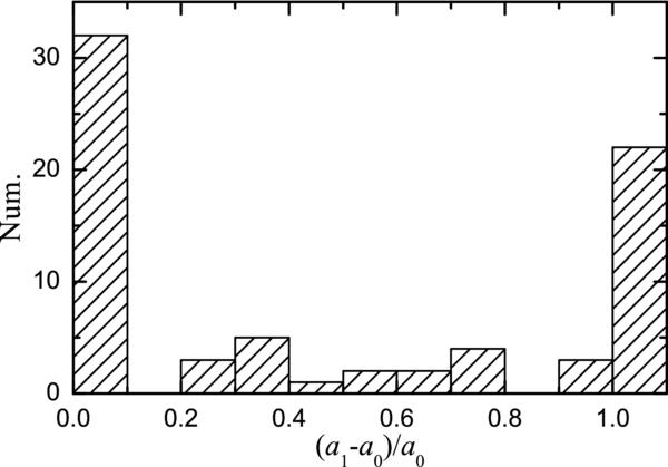
Figure 2. Distribution of a1 − a0/a0 for the 72 SB1s.
Download figure:
Standard image High-resolution imageIt is natural to expect that this approximation should also introduce errors into the other two orbital parameters derived from the revised HIAD, i.e., the inclination and the longitude of the ascending node. Let {i, Ω} and {iJ, ΩJ} be the values of these two parameters obtained by fitting the revised HIAD with and without the constraint a0 = a1, in which case the errors under consideration are simply |i − iJ| and |Ω − ΩJ|. To illustrate the significance of these errors, we compare them, respectively, to the standard errors σi and σΩ shown in Table 2. For this, we plot the histograms of |i − iJ|/σi and |Ω − ΩJ|/σΩ, respectively, in the upper and lower panels of Figure 3. As can be inferred from this figure, more than 30% of the errors introduced by the approximation a0 = a1 are significant at the 1σ level.

Figure 3. Distributions of |i − iJ|/σi (upper panel) and |Ω − ΩJ|/σΩ (lower panel) for the 72 SB1s.
Download figure:
Standard image High-resolution image
In conclusion, we remark that a0 = a1 cannot be taken for granted in the photocentric orbit determination, at least for a few SB1s, by fitting the revised HIAD.
4.2. Comparison with Resolved Relative Orbits
Among the 72 SB1s with a reliable photocentric orbit, there are 3 systems (HIP 65982, 92818, and 112158) resolved by the interferometric observations. By fitting these observations, relative orbits of the components have been obtained (Hartkopf et al. 2012; Hummel et al. 1995, 1998) and listed in the Sixth Catalog of Orbits of Visual Binary Stars (http://ad.usno.navy.mil/wds/orb6.html; Hartkopf et al. 2001). This allows us to measure the likely true errors of our photocentric orbits.
Values of the two orbital parameters derived from the revised HIAD, that is {i, Ω}, can be directly compared with the corresponding values {iI, ΩI} extracted from the relative orbital solutions. In Table 3, all of these values, together with their standard errors, are listed for all three systems. As can be checked for each system, {i, Ω} and {iI, ΩI} are consistent with each other at the 3σ level. This makes us believe that, though our results derived from the revised HIAD are reliable with reasonable precision, they should and could be significantly improved based on ground-based interferometric observations. We will come back to this point in the last section.
Table 3. Comparison between Relative and Photocentric Orbits of Three Resolved Systems
| HIP | iI | i | ΩI | Ω |
|---|---|---|---|---|
| Identifier | (deg) | (deg) | (deg) | (deg) |
| 65982 | 10.0 ± 13.0 | 20.5 ± 3.6 | 135.2 ± 4.5 | 132.5 ± 0.5 |
| 92818 | 40.2 ± 0.6 | 36.1 ± 16.0 | 70.1 ± 1.2 | 86.3 ± 8.1 |
| 112158 | 68.28 ± 0.05 | 65.5 ± 1.4 | 20.9 ± 0.04 | 29.7 ± 6.9 |
Notes. The Hipparcos identifiers of the systems, the inclinations (iI), and the longitudes of the ascending nodes (ΩI) from the relative orbits, and the same quantities (i and Ω) from the photocentric orbits are listed.
Download table as: ASCIITypeset image
4.3. Masses of Components and Semimajor Axes of Relative Orbits
As can be inferred from the spectral types listed in Table 1, there are 25 systems with a main-sequence primary. Under the assumption that the secondary of such an SB1 contributes little to the total luminosity of the system, the primary's mass can be estimated from this luminosity by using the two-piecewise V-band MLR for the main-sequence stars given in Xia & Fu (2010). The piece valid for the mass range 0.60 M☉ < M < 2.31 M☉, or the corresponding absolute visual magnitude range ∼8.99 > MV > ∼ 1.05, i.e.,

is applicable for the present purpose. The absolute visual magnitudes of the above-mentioned 25 systems and the resulting primary masses are listed, respectively, in the second and third columns of Table 4. The relative error introduced to these estimated masses by the above assumption, i.e., the magnitude difference dMV between the primary and the whole system ignored, can be roughly bounded from above. For this, we take the total differential of Equation (5), which gives
For the systems under consideration, MV ranges from 2.00 to 7.18, and so |0.01022MV − 0.125| < ∼0.1. Therefore, |dM/M| < ∼ 10% if |dMV| < 1, which should be true for almost all SB1s.
Table 4. Hipparcos Identifiers, Absolute Visual Magnitudes, Components' Masses, and the Angular Semimajor Axes (a'') of the Relative Orbits of the 25 SB1s with Primaries Being Main-sequence Stars
| HIP | MV | M1 | M2 | q | a'' |
|---|---|---|---|---|---|
| Identifier | (M☉) | (M☉) | (mas) | ||
| 705 | 4.57 | 1.06 | 0.59 | 0.56 | 7.00 |
| 5881 | 5.21 | 0.95 | 0.28 | 0.30 | 30.68 |
| 5952 | 4.53 | 1.06 | 0.28 | 0.26 | 14.81 |
| 6306 | 3.86 | 1.21 | 0.26 | 0.22 | 35.17 |
| 12062 | 5.14 | 0.96 | 0.45 | 0.47 | 35.47 |
| 21433 | 5.66 | 0.88 | 0.24 | 0.27 | 28.68 |
| 22607 | 3.09 | 1.42 | 0.55 | 0.39 | 15.67 |
| 24419 | 5.00 | 0.98 | 0.22 | 0.23 | 57.81 |
| 34164 | 4.07 | 1.16 | 0.70 | 0.60 | 22.71 |
| 39893 | 5.38 | 0.92 | 0.62 | 0.67 | 25.73 |
| 47461 | 2.00 | 1.82 | 1.28 | 0.71 | 16.44 |
| 50966 | 3.18 | 1.39 | 0.61 | 0.44 | 8.48 |
| 51157 | 5.85 | 0.86 | 0.30 | 0.35 | 76.15 |
| 55022 | 3.97 | 1.18 | 0.60 | 0.51 | 16.36 |
| 59750 | 4.40 | 1.09 | 0.48 | 0.44 | 91.99 |
| 63063 | 6.20 | 0.81 | 0.41 | 0.50 | 37.96 |
| 65982 | 5.34 | 0.93 | 0.42 | 0.45 | 95.29 |
| 69442 | 6.01 | 0.84 | 0.52 | 0.62 | 57.65 |
| 73440 | 4.05 | 1.17 | 0.14 | 0.12 | 38.27 |
| 77409 | 7.18 | 0.72 | 0.51 | 0.71 | 29.83 |
| 77801 | 4.89 | 1.00 | 0.14 | 0.14 | 31.31 |
| 82860 | 3.98 | 1.18 | 0.42 | 0.36 | 21.19 |
| 92418 | 3.88 | 1.21 | 0.10 | 0.08 | 34.92 |
| 95028 | 2.98 | 1.45 | 1.19 | 0.82 | 12.85 |
| 99965 | 5.55 | 0.90 | 0.74 | 0.83 | 38.89 |
Download table as: ASCIITypeset image
From the primary masses, secondary masses can be derived by using the mass function
The results are listed in the fourth column of Table 4, and mass ratios (q) are listed in the fifth column.
In order to obtain the precise orbits of the above 25 SB1s, we require further observations, for example, interferometric and double-lined high-resolution spectroscopic observations. For a certain telescope, whether the speckle interferometric observations can be implemented mainly depends on the angular distance between the two components in addition to the components' magnitudes, and the angular distance is proportional to the angular semimajor axis of the relative orbit (a''). Therefore, a'' of the above 25 SB1s is also calculated and listed in Table 4.
5. CONCLUDING REMARKS
The radial velocity and astrometric position are two complementary types of observations constraining, respectively, the binary motion in the radial direction and on the plane of the sky. It is expected that a large number of orbital solutions will be obtained in the near future by assigning reasonable weights to these two types of Gaia data and fitting them simultaneously to the binary model. Nonetheless, the two-step procedure as mentioned in the Introduction (Pourbaix & Boffin 2003; Jancart et al. 2005) will remain useful in determining photocentric orbits at least for some close binaries. This is because the signal strength of radial velocity data is nearly independent of the binary distance and increases with decreasing linear size of the orbit, while that of astrometric data decreases with both increasing distance and decreasing linear size of the orbit, and so, as the considered binary systems become more distant and their linear orbital size becomes smaller, it will not be unusual to encounter the case in which the radial velocity data have significantly larger signal-to-noise ratio than those of the photocenter position. Through the two-step procedure, we have obtained reliable photocentric orbits of 72 SB1s collected in  by fitting the revised HIAD. Some of these orbits are improved with respect to previous ones obtained by fitting HIAD and using the approximation a0 = a1 (Jancart et al. 2005). It is shown that this simplifying approximation is sometimes too crude to be used.
In addition to the upcoming Gaia data, several kinds of present-day ground-based techniques can be used to provide data for improving the precision of our photocentric orbital solutions or giving full orbital solutions. Indeed, by using Doppler Dispersed Fix-delay Interferometry (Mahadevan et al. 2008) or a spectroscopic technique superimposing a reference spectrum, e.g., the iodine absorption spectrum, onto a stellar spectrum (e.g., Konacki 2005; Konacki, et al. 2010), the precision of radial velocity data can reach as high as ∼1 m s−1, several magnitudes more precise than the data used to determine most spectroscopic orbits in  . On the other hand, the resolution ability of long baseline interferometry has been advanced to several tenths of 1 mas (e.g., McAlister et al. 2005; North et al. 2007; Raghavan et al. 2009), one or two magnitudes smaller than the 2a1 for all 72 SB1s listed in Table 2. This implies that most of these SB1s can be resolved since, except for few cases where the brighter component is less massive than the other component, 2a1 is a lower bound of the semimajor axis of the relative orbit. Trying to provide as much information as possible for the relevant observations, we have estimated the mass ratios and the angular semimajor axis of the relative orbit for 25 SB1s with a main-sequence primary.
This research has made use of the SIMBAD database (http://cdsweb.u-strasbg.fr/), the 9th Catalogue of Orbits of Spectroscopic Binaries ( , http://sb9.astro.ulb.ac.be), and the double star library (http://ad.usno.navy.mil/wds/dsl.html). We thank the anonymous referee for instructive remarks, which improved our manuscript. We also thank Dr. F. van Leeuwen for his guidance in using the revised HIAD. This research is supported by the National Natural Science Foundation of China under grant Nos. 10833001, 11073059, 11178006, and 11273066.