

Abstract
Extreme heat, particularly if combined with humidity, poses a severe risk to human health. To estimate future global risk of extreme heat with humidity on health, we calculate indicators of heat stress that have been commonly used: the Heat Index, the Wet-Bulb Globe Temperature and the Wet-Bulb Temperature, from the latest Climate Model Intercomparison Project (CMIP6) projections. We analyse how and where different levels of heat stress hazards will change, from severe to deadly, and how results are sensitive to the choice of the index used. We evaluate this risk at country-level and use population and GDP PPP growth scenario to estimate the vulnerability of each nation. Consistent with previous studies, we find that South and East Asia, and the Middle-East, are highly exposed to heat stress hazards, and that this exposure increases by 20%–60% with global mean temperature change from 1.5 to 3 ∘C. However, we also find substantial increases in heat health risk for some vulnerable countries with less adaptive capacity, such as West Africa, and Central and South America. For these regions, about 20 to more than 50% of the population could be exposed to severe heat stress each year on average, independent of the index used. For global warming of 3∘, European countries and the USA will also be exposed several times per year to conditions with daily mean heat stress level equal to the maximum heat stress of the 2003 heat wave.
Export citation and abstract BibTeX RIS

Original content from this work may be used under the terms of the Creative Commons Attribution 4.0 license. Any further distribution of this work must maintain attribution to the author(s) and the title of the work, journal citation and DOI.
1. Introduction
Many definitions and indices of heat waves have been used in the literature (e.g. [1, 2]). When considering the impact of heat on human health, heat stress (heat transfer between a human body and its environment) needs to be considered. Here we examine three indicators of heat stress commonly used in climate sciences, being the heat index (HI, [3]), the wet-bulb globe temperature (WBGT, [4]) and the wet-bulb temperature (TW, [5]). HI is for instance used by the US National Weather Service to issue warnings, and has been used in epidemiology studies such as [6], whilst the American College of Sports Medicine uses the WBGT to evaluate the risk of outdoor activities. All of these indicators take into account both temperature and humidity, with some also considering other variables (such as the solar radiation for WBGT, although in the rest of this manuscript we focus on its simplified formulation, hereafter WBGT*), but their definition is based on different considerations. For example HI is relevant for a person fully clothed and not perspiring much [7]. WBGT* considers that some skin is wet and exposed, taking into account the wind, solar radiation and cloud cover, and is particularly useful in the context of exercising outside. TW is derived from the law of thermodynamics and it assumes that a person is wet and unclothed.
TW of 35 ∘C has been shown to be the upper limit of human survivability, when the thermoregulation of the inner body becomes inefficient and can lead to heat strokes after a few hours of exposure [8]. Recently, [9] demonstrated, with empirical physiological observations, that the limit of survivability is well below 35 ∘C, and that it varies depending on the environment (humid or dry). Vanos et al [10] also highlighted that this threshold for deadly heat assumes very specific conditions. Based on the simplified formula from [11], corresponding WBGT* level to TW = 35 ∘C can estimated between 46 ∘C and 48.5 ∘C (for hot-dry and hot-humid conditions respectively, as detailed in the supplementary methodology section (available online at stacks.iop.org/ERL/17/064049/mmedia)). As a comparison, [12] defined extreme urban heat conditions at WBGT* = 30 ∘C (using a different conversion between WBGT and HI), which follows the International Standards Organization occupational heat stress threshold for risk of heat-related illness [13]. This highlights that the threshold for deadly heat used here is rather extreme, and much lower thresholds are already considered as dangerous. On a daily timescales, TW has rarely exceeded 31 ∘C in the historical records [14], although some places have experienced hourly peaks above this value [15, 16]. Previous studies have also shown that places such as South and East Asia could reach deadly TW conditions in the future under a 'business as usual' greenhouse gas emissions scenario [17]. Recently, [18] suggested that limiting global warming to  C would likely prevent TW from reaching its deadly threshold over the tropics.
Different heat stress metrics combine the role of temperature or humidity differently. As each variable may be modified differently by climate change, with for example a decrease in humidity in certain regions [19], the estimated future heat stress also varies depending on the chosen index. Some indices reach high values for tropical conditions (hot and humid) whilst others give more weight to dry-hot patterns (typical of mid-latitude heat waves), resulting in differences in the estimated impact on population between indicators. Moreover, it is difficult to directly relate the indices to each other as all vary non-linearly with the temperature and humidity. Recently, [20] have calculated 8 different heat stress metrics from Climate Model Intercomparison Project (CMIP6) data, using a different methodology to compute each index. Unlike the approach used in the present paper, the authors used different thresholds based on several studies for individual indices. Similarly, Smith  [21] used 15 different HIs, some absolute and based on the literature, some relative to the climatology. Here, we use comparable thresholds across all metrics to arrive at an overall estimate of future dangerous heat and then consider mitigation capacity.
This study focuses on population exposure to different heat stress levels at three levels of global warming (+1.5 ∘C, +2 ∘C and +3 ∘C above pre-industrial level), i.e. when the global mean temperature in climate models, driven by greenhouse gas emissions scenarios, reaches these respective levels compared to the preindustrial period. The sensitivity of analyses to the choice of metric is also evaluated and shows that results are robust across metrics except for some dry hot regions. Tropical areas are the most impacted by high heat stress events, especially in low gross domestic product (GPD, in PPP) countries. This is consistent with results from [22]. Higher exposure and lower adaptive capacity in low latitude countries would translate into increased vulnerability [23]. However, some developed countries, such as Qatar or the United Arab Emirates, are also expected to experience severe heat stress regularly, especially at higher global warming levels.
2. Methods
Here, key concepts of the methodology are presented, with equations and more detail provided in the supplementary material.
2.1. Heat stress metrics
All the heat stress metrics used in this study can be approximated by simplified equations based on the dry-bulb temperature (Ta) and relative humidity (RH). For this study, daily means of temperature and humidity are used, thus all indices are also expressed as daily means.
The wet bulb temperature (TW) is based here on an equation from [5], valid for RH between 5% and 99%, and dry-bulb temperatures between  C and 50 ∘C.
For the wet bulb globe temperature (WBGT*), the formulation from [11] is used, which assumes moderately high radiation levels and light wind conditions. WBGT* here denotes this simplified version of WBGT without explicit inclusion of radiation and wind. With this method, values higher than 32.3 ∘C should be considered as dangerous for exercising outside (table 1 from [11]). One must keep in mind that differences exist between the full and simplified formulations, especially for specific hot-humid or hot-dry areas [24]. Results presented in this study are only valid for the simplified version WBGT*.
Finally, the HI is based on the Weather Prediction Center formulation 4 .
2.2. Thresholds for heat stress conditions
Three thresholds are considered for different heat stress levels, namely 'severe', 'dangerous' and 'deadly', and are defined based on the following considerations.
The severe level, based on HI, is derived from the NWS warning system (high incidence of heat cramps, heat exhaustion and heat strokes) 5 and corresponds to about 40 ∘C.
The dangerous level is defined as the high-end of observed heat stress during the historical period, bringing the notion of 'unprecedented events'. This corresponds to HI of 55 ∘C [21] or TW of 31 ∘C [14]. Similar levels of HI have been used in others studies to defined dangerous events (high chance of heat strokes) (e.g. [25–27]), although it is sometimes wrongly referred as a NWS warning level [28].
The deadly threshold is defined based on the potential survivability limit (TW = 35 ∘C, [8]), although this limit is questionable, as discussed in the introduction.
HI thresholds are used as starting points to find T-RH pairs from which corresponding TW and WBGT* values are derived (see supplementary information), except for the deadly threshold which is based on TW value as a starting point. All values are summarized in table 1.
Table 1. Thresholds selected for each heat stress index (in ∘C). Number between brackets correspond to two different estimates based on humid or dry conditions (see section 2.2). Italics indicate the chosen value from which other indices are derived.
| Index | |||
|---|---|---|---|
| Level of heat stress | HI | TW | WBGT* |
| Severe | 40 | 27.5 | 35.5 |
| (26.6–28.4) | (34.8–35.9) | ||
| Dangerous | 55 | 31.0 | 40.5 |
| (30.6–31.6) | (40.3–41.0) | ||
| Deadly | 81 | 35.0 | 47.0 |
| (81–81) | (46.0–48.5) | ||
All figures displayed in the main manuscript are for the three levels of TW (as this index has been frequently used is previous climate studies): severe (27.5 ∘C), dangerous (31 ∘C) and deadly (35 ∘C). Corresponding results using the two other metrics are provided in the supplementary material, and are generally similar.
2.3. Period of analysis
This study focuses on the changes between a reference period and several global mean warming targets. The reference period (REF; 1981–2010) is the most recent period with common data for all datasets used (models and reanalysis). Global mean warming levels considered, relative to pre-industrial period, include: +1.5 ∘C, +2 ∘C and +3 ∘C. This corresponds to global mean warming between REF and the target levels of +0.6 ∘C, +1.1 ∘C and +2.1 ∘C respectively, following the methodology of [29] and using the assessed difference of +0.9 ∘C between 2006 and 2015, and the preindustrial period [30]. The warming targets are identified for each individual model based on their 11-year running mean global mean temperature.
2.4. Datasets
2.4.1. Models
An ensemble of 17 individual models from CMIP6 [31] is selected (supplementary table 2) based on the availability of daily data for Ta and RH and during the whole period of analysis. For each model, the 1980–2014 historical period is extracted and extended from 2015 to 2100 with the SSP370 scenario [32], from which data at the respective warming level targets are selected. This SSP scenario corresponds to medium to high future greenhouse gas emissions and challenging socio-economics development due to regional rivalry [33]. Models forced by this scenario warm at different rates due to differences in their sensitivity, which leads to a range of global mean temperatures by the end of the century [34]. Since this study focuses on change in HIs at specific warming levels (and not to specific periods), results are fairly independent of model sensitivity. All models are linearly regridded on a N96 horizontal grid (about  , corresponding to the lowest resolution of the selected models) prior to further analysis.
We use population projection data from SSP3 [35] and regrid it to the same grid as the models by conservative aggregation on each N96 grid point. The SSP3 gross domestic product based on purchasing power parity (GDP PPP, hereafter simplified as PPP) [36] scenario is used to provide the expected development of a region at country-level. It is used here as a metric to evaluate the potential of a country to take adaptive measures to changing climate hazards. These may include better insulation of buildings, air conditioning, better health care, etc. Lower PPP countries also tend to rely more on farming and outdoor labour, thus increasing the potential exposure to climate hazards.
2.4.2. Model filtering
Prior to analysing multi-model results, we select models (supplementary table 2) based on their performance in simulating the climatology of each studied index during the reference period. A filtering method is used rather than bias-correction to avoid possible bias after correction resulting from heat/humidity nonlinearities.
2.4.3. Reanalysis
To evaluate model performance in simulating HIs during the reference period, 4 reanalysis datasets are used: ERA5 [37], ERA20C [38], JRA55 [39] and NCEP [40]. An estimate of observational uncertainty use the spread of reanalysis data is defined as the maximum of the root-mean square errors (RMSe) between ERA5 and each other reanalysis products. Models with RMSe (against ERA5) larger than the observation error are considered unrealistic and removed from the analysis. Supplementary figure 1 shows reanalysis estimated indices during the reference period. Although this method allows us to select models consistent with reference datasets, one must realise that reanalyses themselves can introduce errors. Particularly, ERA5 and NCEP have been shown to be biased on the cold side [41, 42]. Although results presented hereafter could be impacted by such bias, we reproduced all analysis without model filtering and did not find any major difference.
2.5. Metrics of exposure and vulnerability
Each heat metric is computed by aggregating results from each model and each year (during a certain period). Thus it combines the natural (inter-annual) and inter-model variability. Also note that all variables are computed at each grid cell before eventually being spatially averaged or integrated.
2.5.1. Hazard frequency
The heat stress hazard is expressed in terms of occurrence, i.e. a number of days per year above a given threshold, and is used to quantify how often a population is exposed to hot conditions. The return period is derived from the ensemble sampling frequency and expressed in years.
2.5.2. Population exposure
The exposure is defined by comparing the population and the heat stress hazard occurrence at each grid point. The latter is expressed as a percentage probability for a grid point to have at least one event during a given year. For example, at a given location, if the return period of a chosen threshold is equal to or below 1 year (i.e. average occurrence at least once per year), the exposure is set equal to the local population. If the return period is 2 years (i.e. average recurrence period 2 years) then the average exposure will be set to half of the local population. The population itself corresponds to the gridded dataset from SSP370 at the middle of a decade when the warming level is crossed (thus it is different for each warming level). For the reference period, the population from 2010 is used (corresponding to the beginning of the SSP dataset).
To display results at country-level, the exposure defined above can also be aggregated across each country and divided by their total population. In this case, the country-level exposure is expressed as a percentage of their population, with 100% meaning that each person of a country is exposed at least once per year to a given heat stress threshold.
As a summary, results are also shown as person-days (i.e. multiplying the population by the number of events at each grid point) which is more commonly used in similar studies.
3. Results
First the spatial patterns of changes in heat stress indices are analysed (figure 1). Currently occurrences exceeding TW threshold for severe heat (27.5 ∘C) are mostly confined to the tropics, with yearly or sub-yearly return values. There are also moderate chances for this threshold to be exceeded in some mid-latitude countries such as the Eastern USA, East Asia and Northern Australia. With an increase in global temperature they become more frequent (with sub-yearly return values over most of the tropics) and extend toward the mid-latitudes. For example, the Eastern USA becomes much more exposed to heat stress, whereas the signal remains weak over Western USA at similar latitudes. Higher levels of heat stress are rare today but emerge quickly with global warming. Dangerous events (TW exceeding 31 ∘C), which are currently limited to small areas in the Middle East, are projected to occur over most tropical and sub-tropical countries. They also become possible in Eastern USA at +1.5 ∘C warming and, more rarely, in central Europe at +3 ∘C warming. Deadly events (35 ∘C) emerge at +1.5 ∘C warming over India, South America and Australia, although they remain rare with return values of more than a decade. At higher level of warming, they occur over parts of the USA and many parts of the tropics with return values between decadal to yearly. The three indices exhibit similar behaviour overall (see supplementary material), with some minor differences: High HI values occur more in dry regions (i.e. North Africa or Australia) and have slightly shorter return periods (i.e. events tend to occur more often compared to the two other indices). These differences are larger for deadly events, especially around West Africa. This shows that estimating population vulnerability for the most extreme conditions becomes more dependent on the index chosen, whereas the indices are almost equivalent for less extreme conditions. Also note that in the models dangerous conditions are estimated to not occur during the reference period, when they have been observed very locally [14]. This may be due to the spatial resolution used in this analysis not being high enough to capture very local processes, and that our focus on daily means. Thus our analysis may miss sub-daily and local events of high heat stress.
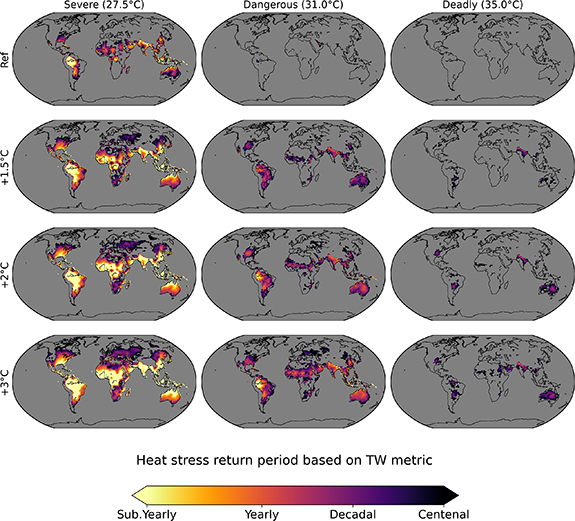
Figure 1. Return period (in years) of heat stress levels, based on wet-bulb temperature, for the reference period (1981–2010) and three different global warming targets. Grey areas indicate masked values (for ocean) or regions without events (for land). Note that here lighter (darker) colours indicate more (less) frequent events.
Download figure:
Standard image High-resolution imageTo assess the population exposure to high heat stress events, the above signals are combined with population estimates at each grid point (see methods). First, the spatially integrated global trend is analysed (figure 2(a)). If global mean temperature reaches +3 ∘C above pre-industrial levels, about 45% of the total population could be exposed each year to severe heat stress (TW = 27.5 ∘C), with an exposure (see section 2.5) reaching around 5 billions. However, if the total population is kept at its current level, global exposure results are very similar (dashed red line). Thus the increase in exposure is mainly due to the increase in heat events and not the change in population. Limiting global temperature increase to +1.5 or +2 ∘C would still lead to about 20% or 30% of the total population exposed to severe conditions, respectively. On the other hand, if following the SSP370 scenario to the end of the century, more than half of humanity could be exposed each year to severe heat stress. Note that the global exposure signal emerges from the variability (grey shading) at +1.5 ∘C global warming (here estimated around 2035 based on the ensemble mean), emphasizing the robustness of projected increase in exposure to extreme heat. Higher heat stress indices show larger uncertainty but also an overall robust increase. At +3 ∘C global warming about 10% of the population could be exposed to TW exceeding 31 ∘C each year, while the exposure to deadly conditions (TW = 35 ∘C) could impact about 100 million people, with potentially severe consequences. Again, there is little difference between the different metrics (supplementary material), although HI shows a slightly smaller ensemble spread. As this index gives more weight to temperature, this narrower spread highlights the fact that model temperatures are probably better constrained than near-surface humidity.

Figure 2. (a) Yearly globally integrated population exposure (as defined in section 2.5) to different levels of heat stress (based on TW): Ensemble mean (black solid line) and 95% confidence interval (grey shading, based on pooling together individual models and years over 10-year windows). The solid red lines show the fraction of the worldwide population exposed to a given heat stress level (right scale). The dashed red line indicates the same as solid red lines but with the population fixed to its present level. The vertical lines indicate the mid-point of the 10-year windows when multi-model mean global mean temperature reaches 1.5 ∘C, 2 ∘C and 3 ∘C above pre-industrial levels, respectively. Note that the exposure scale (left y-axis, with scaling factors at the top of the axes) is different for each plot but the ratio scale (right y-axis) is the same. (b) Percentage of population of each country potentially exposed to different heat stress levels (based on TW metric), for the reference period (Ref) and three different global warming targets (see section 2.5). The scale is different for each heat stress level. Values below 1% are masked.
Download figure:
Standard image High-resolution imageThe country-level exposure is shown in figure 2(b). As pointed out by several studies (e.g. [17, 43]), South and East Asia are two areas with substantial heat stress already at the present time which will amplify with global warming. For example, at +3 ∘C warming the population exposure to severe heat stress is projected to reach more than 10% for most of the countries in this area. Warming is also expected to lead to quickly emerging severe and dangerous conditions in West Africa. At +3 ∘C warming about 80% and 10% of the population in this region will be exposed to TW above 27.5 ∘C and 31 ∘C, respectively. At higher global warming levels most of the world's population will be at risk from severe and dangerous heat, including some mid-latitude countries. A signal of deadly heat events is expected to occur at +1.5 ∘C warming around India, Pakistan and Bangladesh. Despite the rather weak risk (around 1% exposure) the high potential impact and limited time for adaptation is a concern, since this threshold is expected to be reached during the decade centred in year 2035 for the models and emission scenario considered. With further global warming, these events are expected to extend to other countries in South-East Asia and some countries in West Africa, South America and Middle-East. Results based on other indices show a consistent pattern, with HI highlighting also some slightly drier areas (such as North Africa and Middle-East).
Australia shows relatively low population risk from extreme heat, despite the hazard signal shown in figure 1. This is because most of Australia is sparsely inhabited. The largest part of the population is indeed concentrated along the South and East coasts, where heat stress increase is weaker. We caution that given the resolution used in this global analysis, heat hazards near coasts may be underestimated (or poorly represented) due to limited interaction between temperature and humidity. Furthermore, we cannot account for urban effects here, which could amplify heat stress locally. This would require using much higher resolution models, especially where many major cities are located.
A further factor to consider when analysing heat risk is vulnerability, particularly, the ability of a country to mitigate heat risk. Here we use the PPP per inhabitant as a rough measure for adaptive capacity of a country, although we recognize that this incompletely characterizes the complex socio-economic conditions. Other metrics could also be used, such as for example the one used by the World Bank 6 , but it is beyond the scope of this study. PPP is compared to the potential exposure to heat stress at individual level in figure 3.
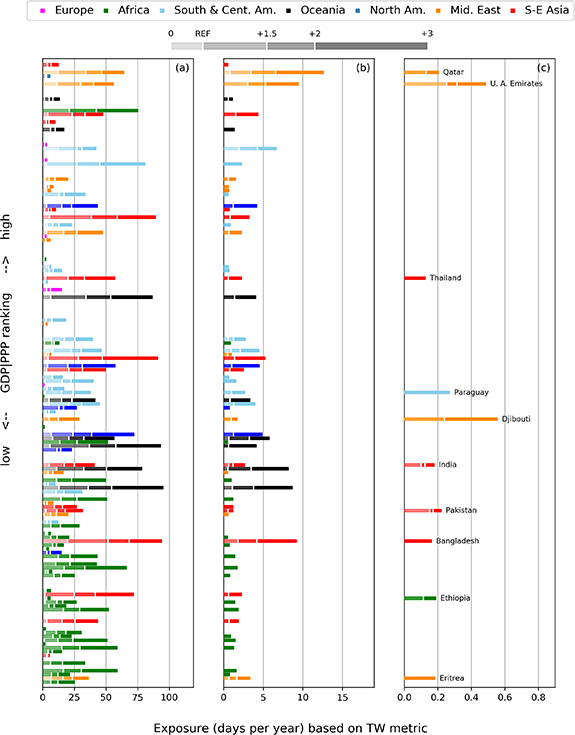
Figure 3. Individual countries exposure (individual horizontal bars), ranked by PPP metric divided by the exposed population, for three levels of heat stress: 27.5 ∘C (a), 31 ∘C (b) and 35 ∘C (c). For each country the total exposure (defined in section 2.5) is also divided by the exposed population. Thus, it indicates for each person exposed to heat stress the number of days per year they would experience different heat stress levels. Each bar shows the exposure for different climate states (as shown by the grey sample bar at the top). Colours correspond to different areas. For the highest heat stress level (c), exposed countries are named. Values below 1, 0.5 and 0.1 are masked in (a), (b) and (c) respectively.
Download figure:
Standard image High-resolution imageExposure to severe heat stress (TW = 27.5 ∘C) is currently limited, but if global warming reaches +3 ∘C nearly all mid and low-latitude countries, including India, will experience exposure for many days per year, with maximum values of almost 100 days per year in Oceania and South-East Asia. This means that people living in exposed areas will have to live under persistent intense heat stress. At that level of warming, many African nations, which represent the poorest and most vulnerable region, show between 25 and 50 days of exposure per year.
Dangerous conditions (TW = 31 ∘C) can also happen every year in many countries. They occur most strongly in the Middle-East, with signals ranging from about 3 to 5 days per year at  C warming to 10–12 days per year at +3 ∘C warming. Other regions are below 10 days per year even at +3 ∘C warming, but the impact could still be considerable in regions with lower mitigation capacity, such as Africa.
Finally, ten nations will potentially be exposed to deadly heat stress, depending on the level of warming. Seven of them are in the bottom half of PPP ranking, meaning that the most vulnerable regions will also be the most at risk. This is consistent with the recent findings of [44], although they used a different exposure index based on monthly mean of daily maximum WBGT. This results is more dependent on the choice of the index. Especially, using HI leads to fewer countries exposed to deadly events, with Qatar, Thailand and Bangladesh being removed from the list (see supplementary), and other countries showing lower risks (for example, U.A. Emirates exposure is 1 day every 5 years with HI, against 1 day every 2 years with TW).
How these changes in heat hazard will translate into impact on population will be related to the level of development each country, with richer nations (such as Qatar) having more resources to adapt compared to poorer countries (for example India, Pakistan and Bangladesh). Also note that exposure per person may be highly unequal within a country, with for example a gradient between the Eastern and Western USA or East China compared to the rest of the country (figure 1).
A summary of previous results, for dangerous events, is given as person-days (taking into account both the population density and the frequency of heat stress events) in figure 4. This shows that exposure to heat stress is consistent across different indices. The most densely populated areas (India and East Asia) have the strongest signal, followed by West Africa, South Asia and South and North–East America. Many of the less developed countries are found in these regions, enhancing the vulnerability of these populations. This metric highlights more local vulnerable areas compared to the country-level exposure (figure 2(b)), meaning that populations can be strongly exposed at regional scale and yet this exposure is underestimated if it is averaged over the country. Different heat stress metrics lead to consistent results but the way the exposure is defined will matter when translating these results to vulnerability or impact.

Figure 4. Exposure to dangerous heat stress levels (TW = 31 ∘C, HI = 55 ∘C, WBGT = 40.5 ∘C) expressed as person-days for each grid point (number of people × number of events). Note that the scale is logarithmic here, from one thousand to 10 millions (and above).
Download figure:
Standard image High-resolution image
4. Conclusion
In this study we compared three commonly used heat stress indices based on a combination of temperature and humidity. We defined three thresholds for each of these indices that correspond to similar heat stress levels (for severe, dangerous and deadly events). We used definitions based on daily mean temperature and humidity model data, implying sustained conditions for many hours. This is different from previous studies evaluating heat stress based on daily maxima only (e.g. [17, 43, 45, 46]). We then evaluated how the frequency of these severe conditions would change at different global warming targets, and how it would translate into population exposure by using the SSP370 scenario (for radiative forcing, population and PPP evolution). The change in heat stress can be related to different contributions of temperature and humidity but in this study we focus only on the combined effect of both variables.
Overall results are robust across metrics, indicating that studies using different indices can be compared for similar heat stress levels. For the most extreme heat stress levels, ensemble results vary slightly more with the index chosen due to different emphasis on humidity.
Our results show that many countries, including mid-latitude ones, could experience severe heat stress events each year at +3 ∘C global warming. This risk would be more confined to the tropics at lower global warming targets, although some areas such as the Eastern USA or South America could also be impacted. Our results also highlight potentially deadly heat stress risk at +3 ∘C global warming.
West African countries will be most vulnerable due to combined high exposure and low mitigation capacity, even if the signal in South and East Asia areas emerges more quickly. There is thus great benefit in limiting global warming to +1.5 ∘C to avoid amplification of West Africa vulnerability.
We also showed that some of the richer countries, especially in Middle-East, could be strongly exposed to high heat stress levels, associated with potentially high economic costs.
A limitation of this study is the use of relatively low resolution model data. While this scale is suitable for large scale temperature patterns, it can lead to an under-estimation of heat stress affected by local processes in regions with complex terrain and high humidity-temperature interactions (such as coastal areas, where localized high humidity values can occur), and it cannot resolve heat stress in urban areas well.
Acknowledgment
This work is supported by the NERC Grant No. 'EMERGENCE', NE/S004645/1. We thank the anonymous reviewers for their careful reading and their many suggestions to improve the work presented in our manuscript.
Data availability statement
No new data were created or analysed in this study.
Footnotes
- 4
- 5
- 6