

Abstract
This study computes the time constants of the temperature elevations in human head and body models exposed to simulated radiation from dipole antennas, electromagnetic beams, and plane waves. The frequency range considered is from 1 to 30 GHz. The specific absorption rate distributions in the human models are first computed using the finite-difference time-domain method for the electromagnetics. The temperature elevation is then calculated by solving the bioheat transfer equation. The computational results show that the thermal time constants (defined as the time required to reach 63% of the steady state temperature elevation) decrease with the elevation in radiation frequency. For frequencies higher than 4 GHz, the computed thermal time constants are smaller than the averaging time prescribed in the ICNIRP guidelines, but larger than the averaging time in the IEEE standard. Significant differences between the different head models are observed at frequencies higher than 10 GHz, which is attributable to the heat diffusion from the power absorbed in the pinna. The time constants for beam exposures become large with the increase in beam diameter. The thermal time constant in the brain is larger than that in the superficial tissues at high frequencies, because the brain temperature elevation is caused by the heat conduction of energy absorbed in the superficial tissue. The thermal time constant is minimized with an ideal beam with a minimum investigated diameter of 10 mm; this minimal time constant is approximately 30 s and is almost independent of the radiation frequency, which is supported by analytic methods. In addition, the relation between the time constant, as defined in this paper, and 'averaging time' as it appears in the exposure limits is discussed, especially for short intense pulses. Similar to the laser guidelines, provisions should be included in the limits to limit the fluence for such pulses.
Export citation and abstract BibTeX RIS
1. Introduction
There has been ongoing public concern about adverse health effects from electromagnetic wave exposure. International standardization bodies have established human exposure safety guidelines/standards (ICNIRP 1998, IEEE-C95.6 2002, IEEE-C95.1 2005, ICNIRP 2010). For frequencies higher than 100 kHz, the thermal effect is dominant (Ziskin and Morrissey 2011, Sienkiewicz et al 2016). According to the international guidelines/standards, the specific absorption rate (SAR) is used as a metric for radiofrequency and microwave exposure for frequencies from 100 kHz to 6 GHz in the IEEE standard (2005) and from 100 kHz to 10 GHz in the ICNIRP guidelines (1998). In the IEEE standard, the frequency range from 3 GHz to 6 GHz is considered as a transition range between using the SAR metric and the incident power density metric. For frequencies higher than 6 GHz and 10 GHz, the incident power density is used as a metric instead of the SAR. In the near future, the frequency range from 6 GHz and up through millimeter waves may be used in fifth-generation (5G) mobile systems. The exposure metrics, i.e. the SAR, electric/magnetic field strength, and power density, should be surrogates of temperature elevation, and thus their relationship has been discussed in earlier studies (Hirata and Fujiwara 2009, Razmadze et al 2009, McIntosh and Anderson 2010, van Rhoon et al 2011).
In 5G mobile systems, little attention has been paid to the thermal time constant in human models for radio frequency localized exposure. According to guidelines/standards, the SAR should be averaged over a 6 min time period for frequencies lower than 3 GHz (IEEE-C95.1 2005) and 10 GHz (ICNIRP 1998). ICNIRP does not formally specify a frequency-dependent 'time' for higher frequencies, but time-dependence enters into the limits in several ways. For example, the ICNIRP far infrared guidelines are stated for 'long term' exposures >1000 s, but only for eye exposure (no comparable long-term limits are stated for skin exposure, particularly for IR-C (ICNIRP 2006). Foster et al (1998) derived an analytic formula to estimate the thermal time constant (although it is defined differently than in the present work) in a 1D homogeneous model exposed to plane waves. In previous modelling studies using anatomical models (Van Leeuwen et al 1999, Wang and Fujiwara 1999, Bernardi et al 2000), the thermal time constant was estimated to be 6–8 min for localized exposure in the frequency bands used for mobile communications (0.8–2 GHz). However, no computations have been carried out for the thermal time constant in anatomical human models for localized exposure over wideband frequencies.
The purpose of this study is to compute the thermal time constants in anatomical head and trunk models exposed to electromagnetic waves from dipole antennas and electromagnetic beams with frequencies that range from 1 to 30 GHz. The temperature elevation caused by localized exposures in this frequency range can be found in Morimoto et al (2016).
2. Model and methods
2.1. Head and trunk models
Both simplified (multi-layer cubes) and realistic (MRI-based) anatomical models were considered. As shown in figure 1, a seven-layer model, consisting of skin, fat, muscle, skull, dura, cerebrospinal fluid (CSF), and brain was considered as the head model, while a four-layer model, consisting of skin, fat, muscle, and intestine, was chosen as the trunk model. The thicknesses of the tissue layers are listed in table 1. The tissue thickness parameters were determined by Drossos et al (2000) and Christ et al (2006).
Table 1. Definition of exposure scenarios: thickness of tissue, model size, and distance of the antenna from the head or trunk models.
| Head | Trunk | |||||
|---|---|---|---|---|---|---|
| Minimum | Average | Maximum | ||||
| Thickness of tissue | Tissues | Thickness (mm) | Tissues | Thickness (mm) | Thickness (mm) | Thickness (mm) |
| Skin | 1.5 | Skin | 1 | 2 | 2.5 | |
| Fat | 1.5 | Fat | 1.5 | 12 | 22 | |
| Muscle | 2.5 | Muscle | 0 | 15 | 30 | |
| Skull | 4.5 | Intestines | Inf | Inf | Inf | |
| Dura | 1 | |||||
| CSF | 1 | |||||
| Brain | Inf | |||||
| Model size | (a) | 70 | (a) | 60 | ||
| (b) | 200 | (b) | 220 | |||
| (c) | 200 | (c) | 150 | |||
| (d) | 25 | 15 | ||||
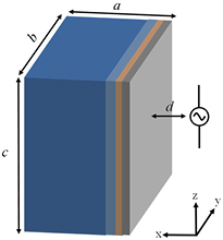
Figure 1. Positions of the feeding points of the dipole antenna relative to a multi-layer cube.
Download figure:
Standard image High-resolution imageMRI-based whole-body voxel models for different ages and races were considered as realistic anatomical models. This study employed the Japanese male model TARO and the female model HANAKO (Nagaoka et al 2004). In addition, two European models of the Virtual Family, Duke and Billie (Christ et al 2010), and NORMAN (Dimbylow 1997) were considered. These models originally had a resolution of 0.5–2 mm, and were segmented into 51–80 anatomical tissues/organs. For head exposure, all the models were truncated at the bottom of the neck because the rest of the body has an insignificant effect on human interaction with a dipole antenna, which will be considered as the electromagnetic field source in this study. In contrast, only the torso was considered for trunk exposure. For models with a resolution of 2 mm, each voxel was divided into 64 smaller voxels with a resolution of 0.5 mm for electromagnetic field simulations with frequencies up to 10 GHz. For the simulations with frequencies above 10 GHz, 2 mm voxels were divided into 512 voxels to give a resolution of 0.25 mm in order to keep the computational accuracy as high as possible. An in-house smoothing algorithm with manual editing was applied in order to maintain the reliability of the models (Nagaoka et al 2005).
2.2. Electromagnetic dosimetry
The finite-difference time-domain (FDTD) method (Taflove and Hagness 2003) was used for numerical electromagnetic dosimetry studies in a human model exposed to microwaves emitted from a dipole antenna. The SAR is defined as

where |E| is the temporal peak value of the electric field at position r, and σ and ρ are the tissue conductivity and mass density, respectively. The dielectric properties of the tissues were summarized in terms of a multiterm Cole–Cole model (Gabriel et al 1996), where the upper frequency at which the measured data were considered was 20 GHz. Measurement at higher frequencies was conducted recently (Sasaki et al 2014a, 2014b). Considering the consistency at lower frequencies, the model by Gabriel et al (1996) was used. The dielectric properties of children's tissues were assumed to be the same as those of adults because after 1 year of age, the variation in human tissues is within a few percentage points across ages (Wang et al 2006).
2.3. Thermal dosimetry
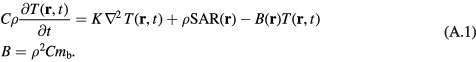
The temperature in the human model is computed by solving a bioheat transfer equation (BHTE) (Pennes 1948). This equation is expressed by the following expression:

where T (°C) is the temperature elevation of the tissue above the baseline temperature (i.e. the temperature above that previous to RF exposure), C (J kg−1 · °C−1) is the specific heat of the tissue, and K (W m−1 · °C−1) is the thermal conductivity of the tissue. B = ρ2C mb (W m−3 · °C−1) is the term associated with blood perfusion, where mb is the volumetric perfusion rate of blood. Further, t is the time evolution in equation (2).
Temperature elevations below the limit of the international guidelines/standards can be considered to be sufficiently small for them not to activate the thermoregulatory response (<6 GHz) (Hirata and Fujiwara 2009). Thus, the blood perfusion rate is assumed to be constant during the computation. Alekseev et al (2005) suggested localized vasodilation using local vasodilator cream and demonstrated its effectiveness for millimeter-wave-induced temperature elevation. Thus, the thermal time constant derived under the blood perfusion rate assumption would be larger than the actual value.
The boundary condition for equation (2) is given by

where H (W/m2/°C), Ts (°C), and Te (°C) respectively denote the heat transfer coefficient, the surface temperature of the tissue, and the temperature of air (23 °C), and n is the axis normal to the body surface.
The BHTE subjected to the boundary condition was first solved to obtain the steady-state temperature elevation and the locations of the maximum temperature elevations in the head tissue (including or excluding the tissues in the pinna), trunk, and brain. Specifically, the left-hand-side term of equation (2) was assumed to be zero and all the right-hand-side terms were independent of t. The equation was discretised using a finite difference method and solved by applying the geometric multigrid method (Laakso 2009). The iteration was continued until the relative residual of the solution was less than 10−7. In the second step, equation (2) was solved in the time domain using explicit time-stepping to follow the temperature elevation at the locations where the peak temperature appeared as confirmed in the first step.
The thermal parameters used in this study are the same as those in Hirata and Shiozawa (2003). These parameters were borrowed primarily from Duck (1990). The heat transfer coefficient between the skin and air and that between the eye surface and air were set to 5.0 and 15 W/m2/°C, respectively, which are typical values at a room temperature of 23 °C (Fiala et al 2001, Hirata et al 2006).
2.4. Exposure scenarios
Exposures of the head (pinna) and trunk to the electromagnetic fields emitted from a half-wave dipole antenna were considered. The positions of the centre of the dipole antenna relative to the pinna and trunk are shown in figures 2(a) and (b), respectively. The antenna lengths were adjusted to resonate at respective frequencies of 151, 76, 51, 38, 31, 25, 21, 17, 14, 13, 8.5, 6.5, and 4.3 mm for 1, 2, 3, 4, 5, 6, 7, 8, 9, 10, 15, 20, and 30 GHz. The dipole was oriented in the up–down (superior–inferior) and front–back (anterior–posterior) directions.

Figure 2. Exposure scenarios using a numeric Japanese male model (computational phantom) in (a) the head and (b) the trunk.
Download figure:
Standard image High-resolution imageIn addition to plane wave exposure (1D analysis), microwave/millimeter beam exposure with diameters of 10, 20, 40, and 150 mm was also considered to clarify the effect of the finite dimension of SAR distribution on the thermal response of the irradiated tissue. Beam exposure in new wireless technologies such as massive multiple-input and multiple-output (MIMO) and 5G mobile systems (Larsson et al 2014, Roh et al 2014) should also be considered in future work.
For these latter simulations, the SAR outside the beam is assumed to be non-existent, i.e. step-like change. Note that an ideal beam with such a small diameter is impossible to produce due to the diffraction limit (comparable to respective wavelengths) at lower frequencies.
2.5. Definition of thermal time constant
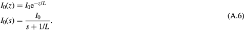
The thermal time constant as used in this study is an empirical quantity that characterizes the time for the exposed tissue to approach the steady state temperature increase after exposure is begun, i.e. the step response of the tissue. It is defined in two cases. The first case is where the time evolution of the temperature elevation is considered as a primary delay function, which was observed in the body surface (i.e. skin in the head and pinna). In this case, the primary delay function is approximated by the following expression,

where Tmax is the maximum temperature elevation and τ is the time constant. The temperature elevation at the thermal time constant is 63% of the maximum temperature elevation because T(τ) = Tmax (1 − 1/e) = 0.63 Tmax when t = τ. It should be noted that the thermal response of tissue to a heat source is only approximately described by a first order response of the form of equation (4); the 'time constant' should only be considered to be a useful parameterization of a nonexponential response. The time constants presented below are calculated separately for major tissues.
In the second case where the time evolution of temperature elevation is considered as a secondary delay function, it is approximated by dead time (heat conduction time) and a time constant of a primary delay function, which was observed in the brain.

where τD is the heat conduction time. Again, equation (5) is only an approximation of the thermal kinetics, which are not strictly described by a single exponential function.
The time constant, in the empirical sense is used here, depends on a number of factors. These include the following.
- Lateral extent of the SAR pattern. The thermal response time will be smaller when the exposed area is small because of the lateral diffusion of heat in addition to heat transfer in a perpendicular direction into deeper tissues. When the exposed area is larger than a few cm2, heat flow will principally be in one direction only, perpendicular to the skin surface, resulting in longer thermal response times.
- Energy penetration depth. The rate of increase in the surface temperature will be slower at lower frequencies because heat is deposited deeper into tissue, resulting in lower thermal gradients at the surface. This will result in a longer thermal response of the surface temperature (Foster et al 2016).
- Thermal resistance in deeper layers of tissue. Much of the heat deposited near the surface has to be conducted into deeper layers of tissue, some of which (i.e. subcutaneous fat) have a lower thermal conductivity than skin.
The BHTE has two intrinsic timescales (τ1, τ2) that represent heat transport by blood flow and heat conduction (Foster et al 1998):

where L is the energy penetration depth into tissue and α is the thermal diffusivity (=K/ρC, about 0.1 mm2 s−1 for skin). The temperature scales τ1 and τ2 come from dimensional analysis of the BHTE. The first of these timescales represents the clearance of heat by blood perfusion, while the second represents the diffusion of heat. The thermal response time of a tissue is a function of these two timescales (see also the appendix) as well as the geometry of the exposed area. A theoretical analysis (see the appendix) shows that the thermal response of tissue to an imposed source of RF heating is not a single exponential function, as shown in equations (4) and (5), although that is a useful approximation.
3. Computational results
3.1. SAR and temperature elevation in the models
Figure 3 illustrates the SAR and temperature elevation distributions on the horizontal plane of the multi-layer cube simulating the head exposed to the electromagnetic fields emitted from the dipole antennas at 1, 6, 15, and 30 GHz. As shown in figure 3, the SAR distribution becomes more localized around the surface of the layered cube as the radiation frequency increases. A similar tendency was even observed for the SAR and temperature elevation distributions in the case of the anatomical head model for the dipole antenna, as shown in figure 4, at the same frequencies as for the case in figure 3, and in the multi-layer cube for beam exposure, as shown in figure 5.

Figure 3. Distribution of the SARs and temperature elevations in the multi-layer model resulting from a dipole antenna: the SAR distribution at (a) 1 GHz, (b) 6 GHz, (c) 15 GHz, and (d) 30 GHz, and the temperature elevation distribution at (e) 1 GHz, (f) 6 GHz, (g) 15 GHz, and (h) 30 GHz. The antenna output power was normalized at 1 W.
Download figure:
Standard image High-resolution image
Figure 4. Distribution of the SARs and temperature elevations in the anatomical model TARO resulting from dipole antenna: the SAR distribution at (a) 1 GHz, (b) 6 GHz, (c) 15 GHz, and (d) 30 GHz, and the temperature elevation distribution at (e) 1 GHz, (f) 6 GHz, (g) 15 GHz, and (h) 30 GHz. The antenna output power was normalized at 1 W.
Download figure:
Standard image High-resolution image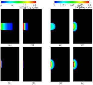
Figure 5. Distribution of the SARs and temperature elevations in the multi-layer model resulting from beam exposure: the SAR distribution at (a) 1 GHz, (b) 6 GHz, (c) 15 GHz, and (d) 30 GHz, and the temperature elevation distribution at (e) 1 GHz, (f) 6 GHz, (g) 15 GHz, and (h) 30 GHz. The incident power density was normalized at 10 W m−2.
Download figure:
Standard image High-resolution imageFigure 6 shows the time evolution of the temperature elevation at the positions where the peak temperature appeared in the head models, including the tissues in the pinna and brain of TARO, for the dipole antenna at the same frequencies as are considered in figure 3. The results with the corresponding seven-layer cube are also shown for comparison. As shown in figure 6(a), the temperature elevation in the outer head increases with increase in frequency. The thermal response time becomes less sensitive to frequency at higher frequencies. For example, for the same incident power density the maximum temperature elevations at 15 and 30 GHz are within 10% of each other, while there are much larger differences between 1 and 6 GHz. This is a simple consequence of very short penetration depths at the higher frequencies, where the exposure approaches the case of purely surface heating. This quantitatively supports the results in figures 3 and 4. As shown in figure 6(b), the temperature elevations in the brain decrease with increase in frequency. Because the energy is deposited closer to the surface of the body it has to diffuse a greater distance to reach the brain, and less heat reaches deeper layers of tissue and it takes longer to arrive.

Figure 6. The time evolution of the temperature elevation in (a) the head and (b) the brain of TARO where the maximum temperature elevation appeared. The antenna output power was normalized at 1 W.
Download figure:
Standard image High-resolution image3.2. Thermal time constant in simplified models
The thermal time constants in different simplified models are computed to clarify their variability. Figure 7(a) shows the frequency dependence of the thermal time constants in simplified head and trunk models: multi-layer head and trunk models and 1D and 3D models. The averaging time of the exposure metrics (SAR, field strength or power density) prescribed in the IEEE standard and ICNIRP guidelines are also compared in the figure. Also shown in figure 7(a) are curves representing the cases with B of 2010 W m−3 · °C−1, corresponding to the 5%-ile value of the skin, (Laakso et al 2017) and 8200 W m−3 · °C−1, shown as the mean value (Hasgall et al 2015).

Figure 7. The frequency dependence of the thermal time constants in layered models simulating the head and trunk. (a) Shows the results for antenna radiation and (b) shows the results for beam radiation. The output power was normalized at 1 W.
Download figure:
Standard image High-resolution imageThe curves for the thermal response time of 1D and 3D homogeneous models are comparable to each other. The difference between the curves depends on the frequency and indicates the effect of the localization of the distribution of the SAR in the direction parallel to the surface of the tissue (figures 3(e)–(h)). As shown in figure 7(b), the thermal time constant is almost frequency-independent for the beam at each diameter, in part reflecting thermal conduction away from the sides of the heated areas. As the beam diameter increases above 40 mm, the thermal time constant reaches a plateau, reflecting the transition to the 1D case, where heat transport occurs chiefly in a direction normal to the surface. Also, at higher frequencies, the energy penetration depth in tissue becomes very short (<1 mm above about 15 GHz) and the heating for all practical purposes is only produced at the surface. Since heat transport also occurs in deeper layers of tissue, it will in part determine the overall step response of the surface temperature.
The above discussion pertains to steady state temperature increases after a constant exposure begins suddenly (the step response). The temperature will approach the steady state after 10–15 min. In addition, as discussed below and in the appendix, if the exposure has time-dependence (i.e. pulsed energy with high peak amplitude but low duty cycle), additional transients will be introduced into the thermal response, which may be significant for extreme exposure conditions.
3.3. Thermal time constants in anatomical models
The thermal time constants in the head models including or not including the pinna and that in the trunk are compared in figures 8(a)–(c), respectively. At each frequency, ten cases are considered, i.e. with two polarizations for each five head models, and the results are processed statistically. The coefficient of variation (CV) (the ratio of the standard deviation of the thermal time constants to that of its mean value) describes the variability of the thermal time constants for the head models, with and without the pinna (figure 9). The same figure also shows the results for five antenna locations on the trunk (i.e. the antenna feeding point was shifted 40 mm in the vertical and horizontal directions) for the TARO and HANAKO models. Note that the effect of polarization is not considered because its effect only produced 5–10% changes in the thermal time constants. The effect of tissue thickness on the thermal time constants is also at most 10%, as shown in figure 8(c), in which its standard deviation for different combination of tissue thickness suggested in table 1 is shown as halftone dot meshing. Thus, different antenna feeding points were considered instead, because this had a bigger effect on the thermal time constants. For comparison, the computed results for the multi-layer cubes, corresponding to the trunk, are also presented in figure 8(c).
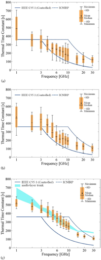
Figure 8. The variability of the thermal time constants of (a) the various head models including the tissues in the pinna, (b) the various head models excluding the tissue in the pinna, and (c) the trunk models. In (c) the standard deviation of the thermal time constants for different combinations of tissue thickness are drawn as halftone dot meshing.
Download figure:
Standard image High-resolution image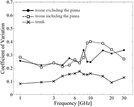
Figure 9. The coefficient of variation for the thermal time constants.
Download figure:
Standard image High-resolution imageAs shown in figures 8(a) and (b), the thermal time constant decreases with frequency, as in the simplified models. At frequencies >10 GHz, the time constants had larger variability, with CV values above 0.35 (see figure 9), particularly in head models that included the pinna. There was much less variability in the time constants for the trunk, and in general the thermal time constants in the trunk are lower than for the head.
The thermal time and heat conduction constants, defined in section 2.5, in the brain are presented in figure 10, and are generally between 310 and 900 s. Since the SAR pattern does not extend into the brain at these frequencies, the thermal response time at the surface reflects in large part the conduction of heat from more superficial tissues. These time constants for the brain generally increase above 4–6 GHz in almost all the models, to approach a constant value above 15 GHz as the SAR pattern becomes increasingly confined to the surface of the head.

Figure 10. The frequency dependence of the thermal time constant in the brain of different head models.
Download figure:
Standard image High-resolution image3.4. Temperature elevation for short pulse exposure
The above discussion pertained to the time taken for the tissue to approach the steady state temperature after a constant exposure begins, i.e. the step response. The response time is rather long because the exposure results, either directly or indirectly, in the heating of a relatively large volume of tissue. A somewhat different, and important, consideration is how to characterize exposure to pulsed energy to provide a useful measure of the peak temperature increase, i.e. how should an 'averaging time' be included in the exposure guidelines? An example of practical interest would be a train of high-amplitude pulses that are separated widely in time, i.e. a pulse train with high peak pulse intensity but low duty cycle. After a brief pulse, the peak tissue temperature will relax to a baseline level due to the diffusion of heat over distances that are comparable to the energy penetration distance into the tissue. This relaxation occurs due to thermal diffusion close to the heated region, and is a much faster process than the approach to steady state after a continuous exposure. This has direct relevance to the setting of exposure guidelines for pulsed energy.
For short intense pulses, the appropriate dosimetric quantity is the fluence (integrated energy density over the duration of the pulse). An upper limit to the peak temperature increase produced by each pulse would be found by considering the response to an infinitesimally short pulse of the same fluence. The time required for the temperature increase to decay to baseline would give a rough estimate of the time over which the exposure should be averaged to allow the peak temperature increase to be captured. In other words, a second averaging time (or an equivalent measure) needs to be specified in the limits for short pulses that is shorter than the 'time constant' discussed above which refers to the step response. In effect, averaging is a lowpass filtering operation. A longer averaging time will capture the thermal response to the exposure averaged over the time, while a shorter averaging time will capture transient temperature increases produced by short pulses. If the pulses carry enough energy to cause injury, such transients are clearly important.
Figure 11 shows the temperature elevation for a beam exposure (diameter of 20 mm) consisting of pulses of 1 and 10 s duration with a constant fluence at different frequencies. For comparison, the steady-state temperature elevation for continuous wave is also shown at an incident power density, which is derived so that its fluence becomes 1000 J m−2 for the duration of the 63% thermal time constant. As shown in figure 11, the momentary peak temperature elevation at the skin surface for short pulse exposure (<10 s) is significant at frequencies higher than 15–30 GHz compared to that produced by a continuous exposure for a given time (63% of the thermal response time) with the same fluence.
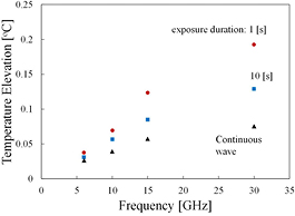
Figure 11. The temperature elevation for beam exposure (diameter of 20 mm) at fluence 1000 J m−2 for different frequencies. For comparison, steady-state temperature elevation is plotted for respective incident power densities, which are derived so that their fluence becomes 1000 J m−2 for the duration of τ.
Download figure:
Standard image High-resolution imageAlthough it is not shown here, the time for the surface temperature to relax to 1/e of the maximum increase after a single 10 s pulse was approximately one-third that of the time needed to approach 63% of the steady state value in the step response: 97, 65, 51, 27, and 19 s at 3, 6, 10, 15, and 30 GHz (see also the thermal time constant for temperature elevation in figure 7(b)). These calculations were performed for small beams (2 cm diameter) and larger differences would be found for larger exposed areas.
4. Discussion and summary
The present study investigated the thermal response in tissues in the human head and trunk exposed to RF energy, including radiation from dipole antennas and beams close to the head. The latter exposure scenario is relevant to new wireless technologies operating in this frequency range, which will eventually include 5G mobile systems.
The computational uncertainty in this study is discussed first. We validated our code in our previous studies, as summarized in Morimoto et al (2016). The major computational error in the FDTD method is due to the discretization, this error depends on the ratio between the model cell size and the wavelength in biological tissue. In this study, the maximum cell size should be smaller than one-tenth of the wavelength to suppress the numerical dispersion error in FDTD simulations; with this condition, the error is less than 10% for the local averaged and whole-body averaged SAR under this condition (Kühn et al 2009, Laakso 2009). The effect of this error on the thermal time constants may be negligible, as can be seen from the analytic solution by Foster et al (1998), but its effect on the maximum temperature elevations is non-negligible. In the thermal analysis, the effect of specific heat and the blood perfusion rate has been assessed based on the analytic solution by Foster et al (1998). All of this discussion and modelling assumes the applicability of the BHTE, which is known to be a reasonable approximation to a decidedly more complex situation in tissue, but is hardly exact (Wissler 1998). As discussed in the appendix, this model is likely to be more reliable when the thermal response is chiefly determined by heat conduction (short timescales, small exposed areas) and less so when blood perfusion (a highly variable quantity) is the dominant mechanism for heat clearance.
As shown in figures 3 and 4, marginal differences with frequency were observed in the temperature elevation distributions for frequencies above 6 GHz. This is largely a result of the concentration of the SAR pattern at the surface at higher frequencies, which approaches the case of purely surface heating, as described in the appendix.
The thermal time constant is defined here as the time required to approach 63% of the maximum temperature elevation. This definition is justifiable because the temperature elevation approximately follows a curve given by equation (4). To verify this, from figure 6(a), the computed time evolution of temperature elevation was fitted with equation (4) and evaluated using the least squares method. The coefficient of determination was 0.998, 0.985, 0.971, and 0.960 at frequencies 1, 6, 15, and 30 GHz, respectively. Similarly, the data from figure 6(b) can be fitted with equation (5) using the least squares method, giving a coefficient of determination that is higher than 0.95 when the value of τD is chosen appropriately. The fitting results suggest that the thermal time constant obtained here is scalable to different temperature elevations. As discussed in the appendix, the overall step response has a complex time-dependence, but its later parts are largely determined by the τ1 (equation (6)) and the approximation of the single time constant response is a reasonable approximation.
As shown in figure 7, the difference between the thermal time constants of the 1D and 3D models was marginal even for the complex tissue geometry near the surface of the head, including the pinna, skin, and subcutaneous tissue. Since Foster et al (2016) and this study used the same theoretical model (Pennes' BHTE) with similar parameters, the more complex results reported here are a result of a more accurate numerical simulation of the body. This study considered 3D models, including anatomically based models. Apart from anatomical detail, the 1D and 3D models differ in their SAR distribution, with the SAR distribution from the dipole antenna localized to a region near the antenna feedpoint. The SAR pattern induced by plane waves in the head model is more uniform across its surface and is more similar to the SAR pattern in the 1D planar model. In addition, the effect of realistic tissue composition was modelled by applying variable thermal parameters to each tissue.
The time constants for the beams with diameters of 40 and 150 mm are similar to those for the plane wave. This is most likely because the heat transfer from the exposed regions in the larger beams is primarily in a direction normal to the tissue surface, whereas for smaller exposed areas substantial diffusion of heat also occurs in a lateral direction (parallel to the surface of the tissue). This may also account for the relative frequency-independence of the smallest beam with a diameter of 10 mm. As discussed in the appendix, the transition from 'small' irradiated areas (where lateral conduction of heat is important) to '1D' models (where heat transfer occurs primarily in a direction normal to the skin surface) occurs at a beam diameter of 10–20 mm, which is consistent with the present results.
From figure 8, the head models differ in their thermal response times above 10 GHz, largely as a result of higher absorption in the pinna, which has a complex shape. The computational results for the anatomical models supported the findings obtained analytically or in simplified models. Our computational results show that the calculated thermal time constants become comparable to 6 min at 4–5 GHz, which is close to the SAR boundary frequency in the IEEE standard and lower than the 10 GHz boundary frequency in ICNIRP guidelines. From figure 10, deep tissues (the brain) have slower thermal response than superficial tissues due to conduction delays for heat from the exposed region to the deeper layers. These conduction delays increase above 4–6 GHz due to the shorter penetration depth of energy at the higher frequencies. In all cases, the peak temperature elevation is smaller in the brain than in the superficial tissue because a considerable fraction of the heat is carried away by blood flow before it reaches the brain.
The thermal time constant calculated in this study is useful in setting exposure limits in that it determines how long it takes for the exposed tissue to reach a steady state in response to an imposed heat source, in effect describing the thermal inertia of the system. This step response is largely determined by the average exposure over the response time. (In a similar way, the thermal response of a large body immersed in water does not depend strongly on momentary variations in the water temperature, provided that they are not too large.) However, brief variations in the input will introduce transients that ride on top of the much slower response. While such short-term transients are normally very small, in some cases (exposure to brief, high intensity pulses) they may be significant. This would indicate the need to put limits on the fluence of brief pulses to limit transient excursions in temperature.
As discussed in section 3.4, the temperature elevation in the skin surface for short-time exposure (<10 s) at constant fluence decays to baseline at a rate that depends on the local temperature gradients. While the response is a complicated function of time (see the appendix), the relaxation occurs over timescales of the order of τ2.
Finally, it is worth commenting that the averaging times in ICNIRP (1998) and IEEE (IEEE-C95.1 2005) were not chosen exclusively on thermal grounds. One consideration is the need to match up the exposure guidelines in the range presently considered to those at lower frequencies (3 or 10 GHz; 6 min) and those contained in laser limits (ICNIRP 2013) at 300 GHz (10 s). For infrared in bands IR-A and IR-B, the limits were designed to protect the cornea and lens of the eye; IR-C (the part of the IR band immediately above the microwave band) had a much shorter penetration depth into tissue. ICNIRP (2006) has limits for 'long term' exposures to the eye (only) of 1000 s (ICNIRP 2006).
The laser guidelines were largely designed to protect humans from intense pulses of infrared energy of duration <10 s, with different limits for the eye and skin. The metric is the fluence (energy density per unit area) over any time period of 10 s. Such waveforms are characteristic of pulsed lasers, and are not typical of wireless communications. However, some technologies exist that transmit intense, brief pulses of millimeter waves, including the US military's Active Denial nonlethal weapons system. Other high-powered millimeter and terahertz pulsed sources are being developed for a variety of non-communications applications and may be sources of occupational exposure in the future. Similar to the laser guidelines, provisions should be included in the limits to limit the fluence of such pulses to limit the transient temperature increases after each pulse. These would be in addition to the limits on exposures averaged over the longer averaging times that apply for continuous exposures (see figures 11 and A2), as discussed in Foster et al (1998, 2016).
The computational results discussed here and related analytical considerations in the appendix will nevertheless be helpful when revising the international guidelines/standards, both of which are currently undergoing revision.
Acknowledgment
The researchers at Nagoya Institute of Technology were supported by the Ministry of Internal Affairs and Communications.
Appendix: Comments on thermal time constants for human exposure to RF energy
This paper presents detailed numerical simulations of the heating effects in the head and torso from RF energy from a dipole antenna located close to it and ideal beam exposure. The main text defines the thermal time constant τ in terms of an exponential response (4) which approximates the step response of the exposed target. This result is useful for empirical characterization of the thermal response. However, theories based on heat transfer analysis do not result in single exponential responses (4).
This appendix considers a simple mechanistic interpretation of the heating of tissue by RF energy as it relates to the more detailed calculations in the main body of this paper, and also as it relates to possible limits for RF exposure.
The following discussion is based on the BHTE given in equation (2) of the main text. For a homogeneous model, the BHTE can be rewritten:
The parameters in the homogeneous tissue are taken from the IT'IS database (Hasgall et al 2015) and used without further modification: K = 0.37 W m−1 °C−1, C = 3390 W s kg−1 °C−1, ρ = 1109 kg m−3, mb = 1.767 ·10−6 m3 (kg−1 s−1), or 106 ml/min/kg in the mixed units typically used in the physiology literature.
This model, based on a simplified form of Pennes' BHTE using standard parameters (Foster et al 2016), provides a good fit to (the sparse) existing experimental data on human thermal response to RF exposure at frequencies from >3 GHz through 96 GHz, with no adjustable parameters. For localized exposures (less than ≈10–20 mm radius) the dominant mechanism of heat clearance is thermal conduction, which is relatively independent of physiological changes; for larger exposed areas the temperature elevation at the skin surface is limited by a combination of thermal conduction and blood perfusion (the latter of which varies greatly with environmental and physiological conditions).
Equation (A.1) has two intrinsic timescales, defined as τ1 and τ2 (equation (6) in the main text), representing rates of heat transfer from blood perfusion and thermal conduction, respectively. For the parameter values used in this paper, τ1 ≈ 500 s and τ2 is a few seconds, depending on the frequency. There are also two distance scales
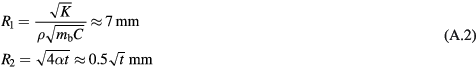
that characterize the distances over which the thermal perturbation from a point source of heat is screened by blood perfusion and thermal conduction, respectively.
Analytical solutions to equation (A.1) are available in the literature, but they are mathematically cumbersome and are not presented here. Over the frequency range considered here, the incident energy is absorbed close to the surface of the tissue, and the exposure situation can be approximated in terms of a model for surface heating only. This approximation is excellent for frequencies >10 GHz. It overestimates the increase in surface temperature by approximately a factor of 2 at 3 GHz. This appendix focuses solely on the case of surface heating. More detailed simulations show that this approximation will overestimate the response to energy with finite energy penetration depths, but not by a large factor for frequencies above 6–10 GHz.
Appendix.
A.1. Step response
We consider an adiabatic plane of tissue exposed to RF energy at an absorbed power density of I0Ttr beginning at time t = 0. We assume that the energy is only absorbed at the surface, but that mb is nonzero. For this model the BHTE has a simple closed form solution (Foster et al 2016):
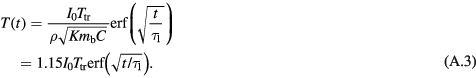
This will reach 63% of the steady state temperature at a time of approximately 0.4 τ1 ≈ 200 s.
Equation (A.3) can be expanded in terms of t/τ1:
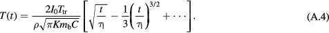
Since τ1 = 1/mbρ, the leading term in equation (A.4) is independent of blood flow, and coincides with the solution for surface heating in a conductive half-plane. Consequently, during the early part of the step response (less than about 100 s after exposure has begun) the dominant mode of heat transport is thermal conduction; the effects of blood perfusion only become significant after a hundred seconds or more when t approaches τ1. This time response shows the characteristic t1/2 behavior of surface heating in a plane due to thermal conduction.
Figure A1 shows the step responses for the adiabatic plane exposed to RF energy at 3 and 30 GHz, which were calculated numerically assuming energy penetration depths appropriate for each frequency. The figure also shows the step response assuming only thermal conduction (mb = 0). For the first 2 min after exposure is begun, the effects of blood perfusion are small, as expected from equation (A.4), and the steady state is approached after several minutes. The response times are similar to those calculated for larger beam patterns in the main text.
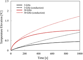
Figure A1. Step response to exposure at 3 and 30 GHz, from a solution to the BHTE assuming the adiabatic boundary conditions and parameters used elsewhere in this paper. The absorbed power density at the surface I0Ttr is assumed to be 60 W m−2. The dotted lines are the corresponding responses for a conduction-only model (no blood perfusion).
Download figure:
Standard image High-resolution imageA.2. Response to pulse
A different time response occurs after a brief pulse. Figure A2 shows the calculated responses to a 10 s pulse at 3 and 30 GHz. The pulse causes a transient rise in surface temperature that decays to baseline after a few tens of seconds as heat diffuses away from the exposed area. The thermal washout in this case takes place on a timescale of approximately τ2, which is much shorter than that characterizing the step response. Consequently, two different timescales are important in characterizing the thermal response of the tissue.

Figure A2. Thermal washout after a single 10 s pulse at 3, 10, 30, and 300 GHz, from a solution to the BHTE assuming the adiabatic boundary conditions and parameters used elsewhere in this paper. The absorbed power density at the surface I0Ttr is assumed to be 60 W m−2. The dashed lines are the corresponding responses for a conduction-only model (no blood perfusion).
Download figure:
Standard image High-resolution image
A.3. Frequency domain analysis
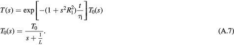
Additional insight into the heating behavior is gained by inspecting the Green function in the (spatial) frequency domain, which is provided by Gao et al (1995). While the Green function is mathematically cumbersome in the time domain, it becomes much simpler in the frequency domain, where the temperature at any point in space (solution to the BHTE) is the product of the Laplace transforms of the Green function with that of the input. While Gao et al (1995) provide the Green function for an infinite medium, that solution can be adapted to the present case (exposure to an adiabatic half plane) by symmetry, since no heat crosses the exposed surface back into space. This requires that the temperature be multiplied by a factor of two from Gao's solution due to the unidirectional flow of heat in the half-plane.
For the case of surface heating, the Green function solution becomes

where T(s, t) and I0(s, t) are the spatial Fourier transforms of the temperature and incident power density, and s is the spatial frequency in m−1. A high spatial frequency indicates spatial gradients in temperature over small distances.
For the step response, I0(s, t) = I0(s)u(t), and the system will approach a steady state temperature that is determined by the first term in parentheses in equation (A.5). The factor (s2 + 1/ ) describes, in engineering terms, a lowpass spatial filter with cutoff frequency 1/R1. This removes spatial frequencies in the temperature above 1/R1, or in other words it describes the effect of blood perfusion to average out temperature variations over distance scales of a cm or so.
For an input I0(z) that decreases exponentially with distance into the plane, we have (ignoring constant factors)
The input has spatial frequency components up to about 1/L. Since L ≪ R1, the input has spatial frequency components higher than 1/R1. In other words, the RF energy is absorbed close to the surface, and the resulting heating pattern has high spatial frequencies.
The approach of the system to the steady state is described by the exponential term in equation (A.5). This term has two factors. The first ( ) is independent of the spatial frequency, while the second (
 ) has a strong frequency dependence and dominates the first factor when s > 1/R1. Both factors also decrease exponentially with time. Consequently, as the temperature approaches the steady state, the high spatial frequency components are quickly lost and the response is dominated by the exponential factor
  . Physically, this occurs because the thermal diffusion quickly smooths out temperature gradients and, over time, thermal equilibrium is produced when heat clearance by blood perfusion balances heat input from the exposure. This accounts for the successful characterizing of the step response in terms of a single exponential despite the fact (equation (A.5)) that the actual temporal response is more complicated.
We now consider now the response to a brief pulse of exposure (thermal washout) (figure A2). We define T0(s) as the surface temperature just after the pulse has ended. If the pulse is sufficiently short for negligible thermal diffusion to occur during it, the temperature profile beneath the surface will be the same as the SAR pattern, i.e. T0(s) = 1/(s + 1/L), ignoring constant factors. The surface temperature will return to baseline after the end of the pulse as
In this case, the relevant timescale of the response is t ≪ τ1. Equation (A.7) lacks the lowpass filter in equation (A.5) and the input T0(s) contains much higher spatial frequencies (i.e. larger temperature gradients over smaller distances) than the steady state temperature distribution. These high-frequency components will decay quickly with increasing time due to the term that is quadratic in s in the exponential factor, while low-frequency components will decay much more slowly. This is seen in figure A2. In the time domain, the transient temperature increases as t1/2 and after a brief pulse the temperature decay will have a larger component that falls off as t−1/2 with a slower decaying component as the low-spatial frequency component decays. This is seen clearly in figure A2.
This has several implications, for the main text and also for setting exposure guidelines. Neither the step response nor the thermal washout are single time constants in behavior, but depend on the spatial frequency content of the input. However, for the step response the 'time constants' obtained from the calculated thermal responses in the main text are useful for describing the thermal response empirically, and describe the later transient response, as shown by the Green function (equation (A.5)). However, the actual time-dependence of the response is not exponential in nature, being closer to that of an error function (equation (A.3)). These comments concern the 1D model. For small beamwidths a 2D model must be used, and the step response time also reflects the lateral diffusion of heat in a direction parallel to the tissue surface.
Thus, there are two different timescales for the problem. The step response occurs over a timescale of approximately τ1, i.e. a few 100 s. This implies that an appropriate 'averaging time' for exposure guidelines would be a few minutes, even at millimeter wavelengths, which captures the average exposure over an appropriate timescale. However, a nonuniform (in time) exposure will also introduce transients in the tissue temperature that quickly decay due to thermal diffusion. There are plausible exposure scenarios involving brief pulses that are intense enough to cause transient increases in skin temperature to hazardous or painful levels (e.g. the US military's Active Denial system).
For exposures consisting of intense pulses at low duty, the simplest, and most conservative, approach would be to limit the fluence (integrated power density during each pulse) to levels such that if all of the incident energy in a pulse were deposited instantly, the maximum increase in the surface temperature would be limited to safe levels. Another, possibly easier, approach would be to define a limit that depends on the square root of the pulse width, to limit the transient increase in temperature to a safe level in accordance with equation (A.5). This would require that the pulses be separated by enough time for skin temperature to return to baseline after each pulse, a few tens of seconds. Consequently, two different averaging times would be present in the limits, one at times in the range of minutes, and a second representative of the duration of pulses.