

Abstract
Frequency modulated thermal wave imaging (FMTWI) has been considered as one of the promising non-destructive testing and evaluation approach due to its merits such as economical, safe, fast, sensitive and high depth resolvability. The present work provides a novel analytical solution for FMTWI using one-dimensional heat conduction equation with adiabatic (Neumann) boundary conditions. The temperature gradient over the glass fiber reinforced polymer specimen has been analyzed and validated with a commercially available three dimensional mathematical finite element model to retrieve the quantitative information regarding the subsurface defects. The efficiency of the proposed method is highlighted using matched filter based approach for a frequency modulated imposed heat flux. The depth resolvability of the proposed method has been studied from the obtained correlation lag and the time domain phase obtained for FMTWI technique.
Export citation and abstract BibTeX RIS

Original content from this work may be used under the terms of the Creative Commons Attribution 4.0 licence. Any further distribution of this work must maintain attribution to the author(s) and the title of the work, journal citation and DOI.
1. Introduction
Thermal non-destructive testing and evaluation (NDT&E) is a reliable, non-contact, whole field testing technique widely used for the assessment of defects such as voids and delaminations. Thermal NDT enables to observe surface temperature gradient on the sample surface using infrared camera to detect presence of any subsurface anomalies. Active infrared thermography (AIRT) is an attractive NDT tool used for detecting flaws caused during various stages from manufacturing to in-service applications [1–3]. The popular optically stimulated active thermal NDT (TNDT) techniques are pulsed thermography (PT) [2–5], pulse phased thermography (PPT) [6–11] and lock-in thermography (LT) [12–14].
PT employs short duration input pulse as heat flux over test sample to measure thermal gradient. Although, PT is a simple and fast technique, its temperature response gets affected due to variations in surface emissivity and non-uniform heating [4, 5] over the test specimen. PPT works on same principle (experimental setup) as PT except the data analysis scheme which is carried out using Fourier transform to extract phase related information from reflected thermal wave. The results obtained from the phase analysis approach are being less sensitive to surface features such as emissivity and non-uniform heating [7–11]. The modulated thermographic technique such as LT utilizes a mono-frequency input thermal excitation of considerably low peak power to compute magnitude and phase information of reflected thermal wave. But LT demands repetition of experiments at different input frequencies to inspect defects located at different depths inside the test sample which make it a time consuming technique [12–14]. Therefore, to overcome the limitations of conventional TNDT techniques such as peak power requirement, penetration depth and resolution, a non-periodic linear frequency modulated (LFM) thermal excitation scheme was introduced.
The fundamental theory of linear FMTWI (LFMTWI) allows heating the test sample with a low peak power heat sources having suitable band of frequencies chosen on the basis of thermal properties and its geometry [15–19]. The thermal waves diffuse into the test sample due to the absorbed heat over the sample. Therefore, a change in surface temperature gradient can be observed in the presence of any subsurface discontinuity. The present paper focuses on the quantitative analysis of the temperature gradient at different depth locations in a glass fiber reinforced polymer (GFRP) sample using a novel analytical tool by analyzing the temperature T(v,t) as a function of position and time observed at the surface v = 0 of test sample. The present paper also emphasizes the time domain Hilbert transform data processing approach using LFMTWI which provides better depth resolution.
The proposed work in this paper has been arranged as follows: section 2 presents principle of LFMTWI technique and analytical solution for heat transfer model under adiabatic boundary conditions. The GFRP sample has been modeled and simulated using finite element modeling software is presented in section 3. Further, time domain data analysis scheme has been explained in this section. Section 4 deals with results obtained from the proposed approach and its comparison with simulated results. Final conclusions are reported in section 5.
2. Mathematical formulation
In LFMTWI, frequency modulated thermal waves diffuses into the test sample within a pre-defined band of frequencies having same energy. This applied heat flux diffuse into the test sample to generate thermal waves and produces a time-varying temperature distribution over the test sample. The existence of sub-surface anomalies may alter heat distribution inside the solid leading to a thermal contrast over the test sample.
The thermal waves generated in a homogeneous finite thickness GFRP sample are studied analytically with the help of a theoretical model. The one-dimensional heat conduction equation describing the temperature distribution without any external source or sink in the test sample assuming constant thermal properties is given by [16]:

where T(v, t) depicts instantaneous thermal profile along spatial coordinate v (m) at time t (s). α denotes thermal diffusivity (m2 s−1) of GFRP sample given by α = kp/ρCp. kp- thermal conductivity (W m−1-K−1), ρ-density (kg m−3) and Cp-specific heat (kJ kg−1-K−1).
Analytical solution for equation (1) was obtained under adiabatic boundary conditions (BC's) i.e. negligible heat flux is exchanged at the other end 'l' of the sample thickness. The heat conduction problem for finite thickness was formulated as per the following time domain boundary conditions:


where To is the test sample initial temperature and W(t) defines LFM input heat flux shown induced at the surface of the GFRP sample expressed as [16, 18]:

where Wo depicts applied heat flux peak value, B is given by B = (fi − fo)/Td is the ratio of difference between initial and the final frequency (bandwidth) to the total duration. The frequency sweep is chosen in order to have large diffusion lengths allowing deep penetration into the entire test sample and Td is the total duration for the applied heat flux.
The fundamental solution of the homogeneous heat conduction equation for finite thickness solid sample by imposing time dependent adiabatic boundary conditions (2–4) is given in the form of:

where

and

where λ are the Eigen values given by; λ = nπ/l with n = 0,1,2,...∞. Each value of λ corresponds to an independent solution satisfying the given heat conduction equation and boundary conditions stated above. П is a new introduced parameter unrelated to t in order to obtain the auxiliary solution. Rn and Sn are the integration constant values obtained by satisfying the initial condition as follows:


where 
The temperature gradient obtained over the sample by neglecting the radiation and convection losses as a function of time at a given depth by applying LFM heat flux is expressed as:
where S represents FresnalS, C represents FresnalC respectively. While acquiring solution for surface temperature T(0,t), the following set of equations has been obtained:

This analytical solution is useful in the analysis of temperature variations at various depth locations as a function of time for identification of subsurface defects presents at any given location v > 0 as shown in figure 1.
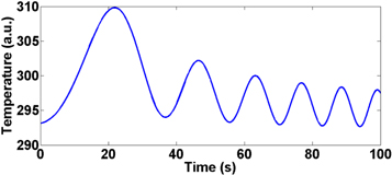
Figure 1. Temperature profile obtained for 0.5 mm depth using equation (12) for incident linear frequency modulated thermal wave input heat flux.
Download figure:
Standard image High-resolution image3. Modeling, simulation & data analysis
The present work explores a finite element method (FEM) based modeling and simulation approach to validate the proposed analytical method. A three dimensional model based on FEM has been designed for GFRP sample having four flat bottom holes each having diameter of 6 mm having thermal properties shown in table 1. The layout of the modeled GFRP test sample is shown in figure 2. Initially, the test sample of finite thickness 0 ≤ v ≤ l is placed at a particular temperature To and while the top surface was subjected to 2 kW LFM input heat flux with a sweep of 0.01–0.1 Hz for a duration of 100 s. The mathematical formulation of the time-dependent heat conduction equation has been considered assuming no internal heat generation within the solid sample. The temperature measurements are recorded at various depths ranging from 0.5–1.2 mm illustrated in figure 2.
Table 1. GFRP sample thermal properties.
| Symbol | Property | Units | Value |
|---|---|---|---|
| kp | Thermal Conductivity | [W m−1-K−1] | 0.3 |
| Cp | Specific Heat Capacity | [J kg−1-K−1] | 1200 |
| ρ | Density | [kg m−3] | 1900 |
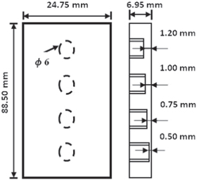
Figure 2. Layout for modeled GFRP test sample.
Download figure:
Standard image High-resolution imageThe temperature gradient was recorded for 100 s duration to validate the proposed analytical method. Additionally, zero mean thermal response for the above mentioned defect depths was formulated by using an appropriate polynomial fitted curve in order to carry out any post-processing technique.
Thus obtained mean removed temperature response is then processed by computing the time domain based cross-correlation (CC) approach between the chosen reference signals (deepest depth) with respect to the other depth locations to determine the potency of relation between the chosen variables. The cross-correlation for the time domain is given as follows:


where R(t) is the reference signal, T(t) is the temperature response for various defect depths, ⨂ denotes correlation, t is the time and τ is the time delay parameter.
These mean removed temperature distribution curves are then used to construct the compressed pulses with the help of cross-correlation technique [19]. The Fourier domain CC was computed between the reference (sound) signal and the temperature recorded for different defect depths given as [20–22]:


where * denotes complex conjugate, ℑ and ℑ−1 denotes fast Fourier transform (FFT) and inverse fast FT (IFFT) between the reference signal R(t) and the defect depths temperature response T(t).
The CC output facilitates the entire energy of the FM signal into a narrow sinc shaped signals of high amplitude. This obtained cross-correlated image enables high depth resolution of the surface and sub-surface defects. The lag time for main lobe and corresponding sample defect depths can be calculated in the form of:

Further, CC-phase for the captured thermal response was obtained using Hilbert transform (HT) where all the frequency components are shifted by an angle of 90 degrees [17, 18].


where RHT is the Hilbert transform of the reference sound signal and sgn denotes the signum function.
The time domain CC-phase can be constructed between the chosen sound signal and captured defect depths given as follows:

The block diagram for constructing the time domain CC-coefficient and phase information using Hilbert transform is shown in figure 3.
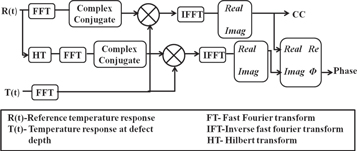
Figure 3. Time domain cross-correlation coefficient and phase image using Hilbert transform.
Download figure:
Standard image High-resolution image4. Results and discussion
An analytical study for the LFM incident heat flux over the surface of the GFRP test sample with frequency sweep 0.01–0.1 Hz for 100 s duration has been carried out. The GFRP sample has four flat bottom holes in the range of 0.5 mm-1.2 mm each having 6 mm diameter is shown in figure 2. The study was carried out under adiabatic boundary conditions and temperature profile for various defect depth locations has been recorded using equation (12) with the thermal properties as given in table 1. Figure 4(a) depicts the analytically obtained thermal responses at different depth locations. Since the obtained thermal profiles have mean (rise) shifted, therefore in order to carry out the proposed post-processing, the zero mean thermal responses have been obtained using the first-order polynomial fit as shown in figure 4(b).
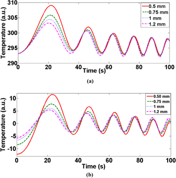
Figure 4. Schematic of (a) temperature response observed from the calculated analytical solution. (b) mean removed temperature response for different defect depths location.
Download figure:
Standard image High-resolution imageThe time domain based CC coefficient approach was adopted on the zero mean temporal thermal profiles to obtain the pulse compression for highly depth resolved imaging of subsurface defects shown in figures 5(a), (b). The CC was calculated for different defect depths of the range 0.5 mm- 1.2 mm in a GFRP sample by considering the 6.95 mm as the reference thermal response.
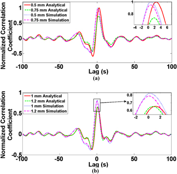
Figure 5. Matched filtering pulse compression profiles obtained using equations (14)–(15) for (a) 0.5 mm and 0.75 mm defect depth, (b) 1 mm and 1.2 mm defect depth.
Download figure:
Standard image High-resolution imageFigure 6 depicts the normalized correlation coefficients calculated for different defect depths for the data obtained from the FEM simulator and proposed analytical solution. It is clear from the trend obtained from the CC-coefficient thermal profiles; there is a significant reduction in the coefficient values as a function of depth.
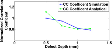
Figure 6. Normalized CC-coefficients obtained from FEM based simulator and analytical model for different defect depths.
Download figure:
Standard image High-resolution imageFurther, time domain based phase information is retrieved by the Hilbert transform based post processing to reconstruct the imaginary component of the reference temperature distribution for analyzing the phase response for LFMTWI as shown in figure 3. Finally, depth resolvability for LFMTWI was demonstrated in figures 7(a), (b) in terms of (a) CC-lag and (b) CC-phase while keeping reference as 6.95 mm thickness of GFRP test sample.

Figure 7. (a) Depth resolvability of LFMTWI for defect depths in terms of cross-correlation lag time (in ms). (b) Depth resolvability of LFMTWI for defect depths in terms of cross-correlation phase (in degrees).
Download figure:
Standard image High-resolution image
The results depicted in figure 7(a) indicate high depth resolvability for the computed analytical solution in comparison to the FEM based simulator. The CC-lag time (ms) induced to the presence of defects in the GFRP test sample calculated from equation (18) decreases with the increase in depth and converge to zero for the deepest defect.
Furthermore, the CC-phase contrast for LFMTWI model is depicted in figure 7(b) for FEM simulator and proposed solution. A lower phase value was observed initially for the shallowest defect and then leads to higher phase value with the increase in defect depths. The presented results suggest its capability for better or comparable defect depth resolvability for LFMTWI input heat flux.
5. Conclusion
The present paper highlights a novel analytical treatment for LFMTWI and validated with the commercially available FEM software with adiabatic BC's which can be treated for practical experimental scenario. The results obtained for a GFRP test sample having four flat bottom defect holes are considered and the proposed post-processing schemes have been analyzed to prove the defect detection capabilities of the FMTWI. Depth resolvability for the above solution in terms of cross-correlation coefficient and its resultant time lag and phase are discussed. Furthermore, the provided analytical representation has been validated with the numerical results obtained from the three dimensional finite element models to prove the applicability of the proposed analytical model.
Data availability statement
No new data were created or analysed in this study.