

Abstract
A crucial prerequisite for a detailed interpretation of the experimental results obtained with the most common attosecond spectroscopic techniques is a careful characterization of the attosecond extreme-ultraviolet (XUV) and femtosecond infrared (IR) pulses used in the measurements. A commonly adopted approach is based on the measurement of the spectra of the photoelectrons produced by the interaction of the attosecond pulses with a noble gas in the presence of a delayed IR pulse. Feeding the resulting spectrogram to reconstruction algorithms, it is then possible to retrieve the temporal properties of the XUV and IR pulses. To date, all reconstruction techniques are based on the assumption that the spectrogram is produced by the interaction of a single atom with a two-color (XUV-IR) field. In this work, we numerically investigate the effect of the actual XUV and IR beam spatial distributions, and we analyze their impact on the retrieval of the temporal characteristics of the XUV and IR pulses and on the determination of the photoemission time delays. We show that the impact of the ensemble effects can be severe, leading to notable variation of the photoelectron spectrograms, depending on the ratio between the XUV and IR beam spot sizes and on the IR peak intensity. We demonstrate that the photoemission time delay can be retrieved with great accuracy even in the presence of large deformations of the photoelectron spectrograms by employing suitable reconstruction procedures.
Export citation and abstract BibTeX RIS

Original content from this work may be used under the terms of the Creative Commons Attribution 4.0 license. Any further distribution of this work must maintain attribution to the author(s) and the title of the work, journal citation and DOI.
1. Introduction
During the last two decades, continuous progress in attosecond technology opened the way to the investigation of fundamental processes in matter [1–4], for example the charge migration in molecules [5, 6], the temporal delay in photoemission from atoms [7, 8], the ultrafast dynamics in the process of photo-ionization [9], with particular attention to photoemission from solid targets [10–12], to name just a few of them. Several experimental techniques have been introduced for the characterization and application of attosecond pulses [1, 13, 14]. The typical experimental approach is based on the use of attosecond pulses in combination with few-femtosecond infrared (IR) pulses. One of the most used spectroscopic schemes is time-resolved photoelectron spectroscopy, in which extreme-ultraviolet (XUV) attosecond pulses are used to ionize the sample, and intense (1011–1012 W cm−2) IR pulses probe the response by modifying the final energy of the photo-emitted electrons. The photoelectron spectra are then collected as a function of the XUV-IR time delay forming a spectrogram. This is the experimental technique commonly used for the temporal characterization of attosecond pulses, in the form of a train of pulses or isolated pulses. In the case of trains, the spectrogram is often analyzed using the reconstruction of attosecond beating by interference of two-photon transitions (RABBITT) technique [15, 16], from which the average attosecond pulse can be estimated. More generally, the spectrogram can be treated with a reconstruction algorithm using a FROG-CRAB (frequency resolved optical gating for complete reconstruction of attosecond bursts) approach, which is based on the strong field approximation [17]. In the case of isolated pulses, the corresponding spectrogram is called attosecond streaking trace [18] and the FROG-CRAB method can deliver a complete temporal characterization of both the XUV and IR pulses. Attosecond streaking has also been successfully employed in attosecond metrology, for example, for the study of the timing of the photoemission process [7, 19]. As important physical effects are encoded in small photoemission delays [20–22], being able to disentangle the fundamental phenomena happening during photoemission in complex systems calls for a more and more accurate temporal characterization of the attosecond pulses involved.
To date, all reconstruction algorithms implicitly assume that an experimental streaking trace results from the interaction of a single atom with a two-color (XUV-IR) field with uniform radial intensity distribution. In this work, this procedure will be referred to as 1D approach (or 1D approximation). However, in a realistic attosecond streaking setup, an ensemble of atoms interacts with XUV and IR fields, each characterized by a given radial intensity distribution. Moreover, the interaction occurs within a finite volume, dictated by the characteristics of the electron spectrometer used for the measurement of the spectrogram, thus questioning the validity of the 1D approximation. To our knowledge, the reconstructions of experimental data reported in the literature have always disregarded these ensemble effects. A reliable and detailed characterization of both XUV and IR pulses is crucial for a correct analysis of the ultrafast dynamics initiated by attosecond pulses. Furthermore, theoretical modeling of the attosecond experiment often requires a detailed knowledge of the temporal and spectral properties of the radiation used. For these reasons, the investigation of the influence of the spatial distribution of the XUV and IR pulses on the reconstruction of their temporal characteristics is important for the attosecond and ultrafast spectroscopy communities.
In this work, we numerically investigate the effects of a non-uniform radial intensity profile of the XUV and IR pulses on the photoelectron spectrograms and on the reconstruction of the temporal and spectral characteristics of the two pulses. We will first calculate the spectrograms resulting from the photoelectrons generated by atoms located on a plane perpendicular to the propagation direction of the two-color field (2D approach). Then we will consider an ensemble of atoms within a finite volume (3D approach). The effects of the ensemble averaging on the reconstructed temporal characteristics of XUV and IR pulses will be investigated in section 3, in the 2D and 3D scenarios. For the reconstruction of both pulses, we employed the extended ptychographic engine (ePIE) algorithm [23]. In section 4, we will investigate how the estimation of the photoemission time delay is affected by the ensemble effects. In particular, the relative photoemission time delay between two species (argon and neon) is calculated from two spectrograms by employing a modified version of the ePIE algorithm, able to reconstruct in parallel both streaking traces by fixing a unique IR pulse, thus guaranteeing a unique time reference for all fields.
2. Methods
Within the strong field and the wavepacket approximations the photoelectron spectrum (called spectrogram),  , is given (in atomic units) by [24]

where p is the final electron momentum, τ is the temporal delay between the XUV and IR pulses,  is the gas ionization potential,
  is the temporal phase imposed by the IR field to the electron wavepacket generated by the attosecond pulse in the continuum. This phase modulation is given by

where  is the vector potential of the IR field.
  is the electron wavepacket, defined as [25]

where  is the inverse Fourier transform operator. The electron wavepacket contains information on both the electric field of the XUV pulse,
  , and on the atomic species involved in the interaction, by means of the dipole transition matrix element from the ground state to the continuum,
  , which can be written as

where  is the cross-section associated to the photoionization probability and
  is the phase acquired by the electron during the ionization process [26]. From the spectrogram (1) it is possible to retrieve the temporal characteristics of both XUV and IR pulses. Equation (1) describes the interaction of an atom with the XUV and IR pulses, without considering their spatial intensity distributions. In the following, this approach for the calculation of the spectrogram will be referred to as 1D approximation. Assuming that the XUV and IR pulses are linearly polarized along the x axis (see figure 1) and that we can neglect angular effects from the dipole element already discussed in [27], we can re-write equation (1) as a function of the final kinetic energy of electron
  , hence expressing it as
  .
.
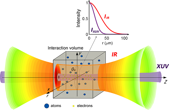
Figure 1. Schematic plot of the interaction between XUV and IR pulses with an ensemble of atoms. The inset shows the radial intensity profiles of the two beams at  .
.
Download figure:
Standard image High-resolution imageIn an actual experiment, however, an ensemble of atoms is subjected to a non-uniform spatial distribution of the light pulses in a finite interaction volume, as sketched in figure 1. As a result, the recorded photoelectron distribution is a collection of electrons emitted by the ensemble of atoms. In classical terms, each photoelectron of each atom is emitted at a specific time-space position and then propagates in free space, experiencing, during the whole process, different values of the two-color (XUV-IR) fields. The resulting spectrogram can be calculated as an incoherent sum of different spectrograms, generated by the interaction of the two-color field with atoms located in points with coordinates  , where r and θ are the polar coordinates and z is the coordinate along the field propagation axis, as shown in figure 1. Therefore, the photoelectron energy distribution,
  , is calculated as

where  is calculated by using equation (1) with
  and
and  evaluated at the streaking points
  .
.
As the XUV and IR pulses are linearly polarized, their electric field can be written as

where ex
is the unitary vector of the x-axis and j = XUV, IR. In the simulations,  has been assumed as Gaussian. Transform-limited (TL) IR pulses were used in the simulations, with a full-width at half maximum (FWHM) duration of 5 fs. In order to take into account the group delay dispersion (GDD) of the XUV pulses, in this case we have first defined the electric field in the frequency domain as

where ω0 is the central angular frequency of the XUV pulse and  is related to the TL-duration of the pulse (FWHM of the temporal intensity profile),
  , by the following relation:
  (in this work we used a TL-duration
  as). For what concerning the spatial distribution, we assumed a Gaussian spatial profile for the XUV pulse. In a streaking experiment, the IR beam is typically reflected by a hole-drilled mirror, thus acquiring an annular shape, and it is focused on the gas target collinearly with the XUV pulse, by a mirror with focal length f (in the simulations, we assumed a 1.5 mm hole diameter and a focal length
  mm). Knowing the geometry, the evolution of the transverse profile of the IR field along the propagation axis can be calculated numerically by using the Fresnel diffraction integral (as reported in [28]).
The main characteristics of the XUV and IR pulses used in the simulations are listed in table 1.
Table 1. Pulse parameters used in the simulations. TL duration: transform-limited duration; GDD: group delay dispersion; D0: FWHM spot size in the beam waist;  .
.
| XUV | IR | |
|---|---|---|
| TL duration (FWHM) (fs) | 0.25 | 5 |
| GDD (fs2) | 0.01 | 0 |
| D0 (µm) | 50 | 50η |
| Central wavelength (nm) | 24.24 | 800 |
The FWHM size in the beam waist of the XUV radiation is  m, where
  is the corresponding spot size at the beam waist, while the IR beam has a FWHM-size in the beam waist
  (with
(with  ). It is evident that the limit
  formally corresponds to the 1D approximation, which will be used as a reference to evaluate the impact of ensemble effects quantitatively. The energy axis of the simulated final photoelectron trace has a resolution of 0.01 eV, and the time resolution is 5 a.s. The choice of the delay axis resolution is not a strong constraint for ptychographic algorithms, as proved in [29], so it was set at 100 a.s. In all simulations, we have implicitly assumed a homogeneous gas density. We have first calculated the spectrograms resulting from the interaction of the two-color field with atoms distributed onto the
  plane, considering the radial variation of the fields, upon changing the IR pulse intensity and the spot size ratio, η. This approach for calculating the spectrograms will be referred to as 2D approximation. The spatial profiles of IR and XUV beams have been sampled over 20 radial points. A second set of simulations have been performed considering the contributions to the streaking trace of the photoelectrons ejected inside a three-dimensional interaction region around the IR and XUV beam waist (hereafter, 3D approach). In this case, the spatial grid was composed of 60 z-points sampled over 3 mm, which is a typical experimental window for a time-of-flight spectrometer used to collect photoelectrons in streaking experiments [30]. For each z point, a 2D simulation was performed.
3. Ensemble effects on the reconstruction of pulse characteristics
3.1. 2D approach
Figure 2(a) shows the spectrogram calculated in argon, at  (beam waist), assuming an IR peak intensity
  W cm−2, at the limit
  (1D approximation). Figure 2(b) displays the spectrogram calculated in the same conditions, but considering the radial variation of the two-color field (2D approach), assuming
  .
.
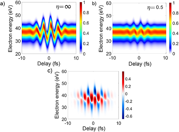
Figure 2. Streaking trace,  , calculated in argon at
  , assuming the pulse parameters listed in table 1, an IR intensity
  W cm−2 and (a)
  (1D approach), (b)
  . (c) Difference between the spectrograms reported in (a) and (b).
Download figure:
Standard image High-resolution imageThe spectrogram is notably affected by the ensemble effects, with an overall energy smoothing of the trace and a clear reduction of the maximum streaking amplitude, due to the averaging over different streaking points that feel a local IR peak intensity lower than in the 1D approximation. As shown in figure 2(c), the maximum deviation with respect to the 1D spectrogram, i.e. max![$[S_\mathrm{1D}(\mathcal{E},\tau)\,-\,S_\mathrm{2D}(\mathcal{E},\tau)]$](https://content.cld.iop.org/journals/2515-7647/4/3/034006/revision2/jpphotonac7991ieqn42.gif) is ∼60%. In the worst case scenario (
is ∼60%. In the worst case scenario ( W cm−2,
  ), this value reaches ∼80%.
The extent and severity of the ensemble effects on the streaking trace depend on the IR peak intensity and on the spot size ratio η, as reported in figure 3(a), which displays the average standard deviation between the 1D and 2D spectrograms,

as a function of η, for four values of the IR peak intensity, ranging from  W cm−2 to
  W cm−2. In equation (8) N and M are the 2D matrices dimensions.

Figure 3. (a) Maximum deviation between 1D and 2D spectrograms ( ),
),  equation (8), as a function of the spot size ratio, η, for four values of the IR peak intensity. (b) same as (a) but as a function of the IR peak intensity.
Download figure:
Standard image High-resolution imageAs shown in figure 3(a), the maximum deviation decreases upon increasing η. This behaviour is related to the fact that, upon increasing η, the XUV spot size becomes significantly smaller than the IR spot size, thus reducing the radial variation of the IR intensity experienced by the atoms interacting with the XUV pulse. As shown in figure 3(b), the deviation increases with IR intensity. At a given η value, stronger IR fields induce a stronger streaking amplitude in the spectrogram. In addition, also the pulse tails become intense enough to influence the electron momentum significantly. Consequently, the 'interaction area' in the trace increases and the smoothing operated by the radial average has more severe effects.
Apart from the variations on the spectrogram qualitatively discussed above, it is important to analyze the effects on the reconstruction of the IR and XUV characteristics. In this regard, particularly relevant are the retrieved XUV and IR time durations, as well as the IR peak intensity. While the former two define the achievable time resolution, the latter identifies the interaction regime (e.g. multi-photon vs. field amplitude driven [31]) which establishes when the IR pulses are used as pump in a time-resolved experiment. Starting from a simulated spectrogram, these quantities can directly be evaluated from the reconstruction output, as it is routinely done with experimental streaking traces. We found the reconstructed IR time duration, defined as the full-width half-maximum of the pulse intensity profile, to be largely insensitive to 2D ensemble effects.
Figure 4(a) shows, on a logarithmic scale, the IR peak intensity, as  , retrieved with directly evaluated using the IR field reconstructed by the ePIE algorithm when fed with the streaking traces calculated within the 2D approximation. The retrieved IR peak intensity is severely affected by ensemble averaging when
  . In this case, the retrieved IR peak intensity is underestimated by more than one order of magnitude. Upon increasing η, the reconstructed IR intensity asymptotically approaches the correct value, shown by horizontal dashed lines in figure 4(a). These results are a direct consequence of the ensemble averaging process. In fact, the reconstructed IR intensity is now an average over many streaking points, each simulated with a maximum intensity always lower than the peak one.
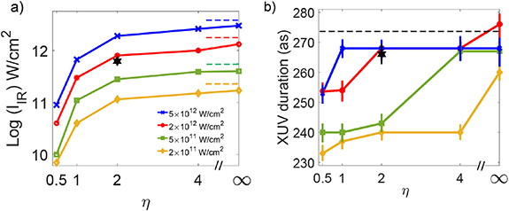
Figure 4. (a) Reconstructed IR peak intensity from a set of 2D simulations as a function of η, obtained with ePIE reconstructed IR electric field. The colored dashed lines on the right part of the plot represent the simulated intensity values. (b) Reconstructed XUV FWHM duration extracted from the simulations reported in (a), from ePIE algorithm. The error bars are proportional to the standard deviation obtained by feeding the algorithm with 6 different initial conditions of the IR duration (from 4 to 10 fs). The black dashed line represents the XUV FWHM duration used in the simulation. Black stars in (a) and (b) are the results of 3D simulations, assuming  and
and  W cm−2.
Download figure:
Standard image High-resolution imageFigure 4(b) displays the duration of the attosecond pulses retrieved by applying ePIE reconstruction to the spectrograms calculated using the 2D approach, as a function of η for four values of the streaking pulse intensity. Also this quantity is affected by ensemble effects, with an error on the reconstructed duration of almost 40 as, corresponding to a ∼ relative error. The dependence of the reconstructed duration on η and IR intensity is rather complex. In general, the reconstruction of the XUV pulse duration improves upon increasing η and the IR intensity. However, at high intensity (
 W cm−2), the precision of the reconstruction procedure gets worst, as highlighted by the increasing error bar size of the blue curve in figure 4(b).
3.2. 3D approach
Assuming an XUV FWHM-spot size at the beam waist  m (see table 1), the corresponding Rayleigh length is
  mm, much longer than the interaction region contributing to the measured photoelectron spectra,
  mm. Therefore, the effect induced by the variation of the XUV intensity along the z-axis is entirely negligible. Figure 5(a) shows the spectrogram calculated in argon using the parameters reported in table 1 assuming
  and a streaking peak intensity
  W cm−2. The corresponding Rayleigh length of the (annular) IR beam is
  mm. We assumed an interaction region extending from
  mm to
mm to  mm. Figure 5(b) displays the difference between the two spectrograms calculated within the 3D and 1D approach, while figure 5(c) shows the difference between the two spectrograms calculated within the 3D and 2D approaches. While the maximum difference between the 3D and 1D spectrograms is of the order of
  , the difference between the 3D and 2D spectrograms is quite small, with a maximum value of the order of
  , thus suggesting that, at least with the pulse parameters of the simulations, the primary role is played by the 2D-ensemble averaging. For this reason, the IR peak intensity and the XUV pulse duration retrieved from the 3D spectrograms are close to the values obtained using the 2D approach. This is shown in figures 4(a) and (b) for a particular value of η and
  (black star).
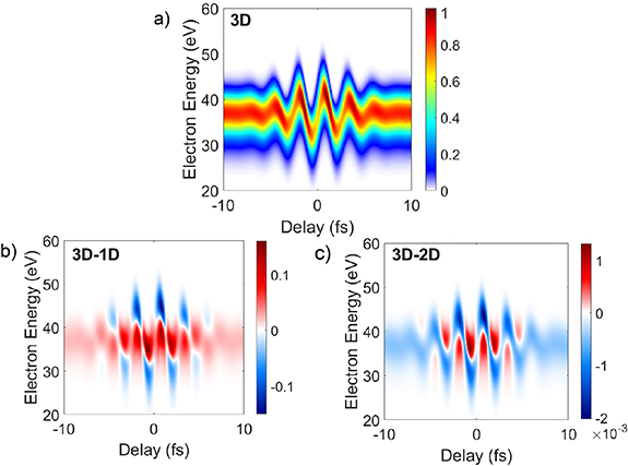
Figure 5. (a) Streaking trace,  , in argon calculated using the 3D approach, using the parameters listed in table 1 and assuming an IR peak intensity (in z = 0)
  W cm−2 and a spot size ratio
  . (b) Difference between the 3D and the 1D spectrograms. (c) Difference between the 3D and the 2D spectrograms (the 2D spectrogram was calculated in
  ).
).
Download figure:
Standard image High-resolution imageSince the Rayleigh length of the IR pulse is significantly longer than the interaction region, we expect that the intensity variation along the propagation axis induces negligible effects. Therefore, the differences between the 3D and 2D approaches can be mainly ascribed to the z-dependence of the Gouy phase. The role of the Gouy phase, at a given z position, is to shift in time the carrier-envelope phase (CEP) of the IR with respect to its value at z = 0. Due to Gouy phase averaging, the resulting 3D-trace is generated by summing different 2D-streaking simulations, each one with a CEP-shifted IR. The maximum shift summed in the average depends on the maximum Gouy phase variation over the considered integration window. In the case considered for the simulations reported in figure 5, the largest shift is 120 a.s. The CEP shift present in the IR temporal profile thus causes a direct CEP-shift in each streaking point at different z-position. As a result, we observe both a vertical broadening of the 3D-trace due to the sum, at a fixed delay, of 2D-traces which experience a different IR radial intensity and a horizontal broadening, due to a z-dependence of the IR CEP.
4. Photoemission time-delays
We have then analysed the effects induced by the 2D and 3D approaches on the determination of photoemission time delays, which, under the right experimental circumstances [19], can be reconstructed from the streaking trace. Without a priori knowledge of the XUV temporal properties it is only possible to extract the relative photoemission time delay between two atomic species, for example argon and neon,  [20]. We developed an upgraded version of ePIE that reconstructs in parallel the streaking traces calculated in argon and neon, by fixing a unique IR pulse. With this approach it is possible to extract simultaneously the two fields,
  and
and  in argon and neon, respectively, and the IR electric field,
  . This method guarantees a unique time-reference for all the fields and allows us to disentangle the XUV phase from the atomic information, which otherwise would be impossible to extract from a single two-color interaction experiment. By using equations (3) and (4), the ratio between the Fourier transforms of
  and
and  can be written as
The phase term in equation (9) contains the relative photoemission time-delay,  , as a function of the photon frequency [32]:

The solid lines in all panels of figure 6 show the relative photoemission time delay,  , calculated by using the atomic dipole phases,
  , of both atomic species reported in literature [33]. The dashed curves in figure 6 display the relative photoemission delay, calculated by using the atomic dipole phases retrieved from the spectrograms obtained in argon and neon using the 2D approach for four different values of the IR peak intensity. In all simulations, we included the photo-ionization cross-sections, reported in [34].

Figure 6. Photoemission time-delay difference  calculated using the 2D approach, for different values of η, and for different IR intensities, ranging from
  W cm−2 to
  W cm−2. The shaded areas represent the reconstruction error evaluated by starting from six different IR initial guesses with duration between 4 and 10 fs. Black solid curves show
  calculated by using the atomic dipole phases reported in literature [33].
Download figure:
Standard image High-resolution imageAt each IR intensity, five spot-size ratios were considered. The black solid curve in figure 6 corresponds to the theoretical values of  . In the case of low IR intensity (
 W cm−2), reported in figure 6(a),
  is only slightly affected by the 2D ensemble averaging. Weak deviations from the 1D-case (
 ) are present at the edges of the energy region of interest (42–64 eV), outside of which the reconstruction is unreliable as the spectral intensity is very low. Similar trends are reported in the medium intensity regime (
 W cm−2 and
  W cm−2), shown in figures 6(b) and (c), where the deviation from the 1D case increases upon decreasing η. The larger deviation from the theoretical value observed at lower photon energies when
  W cm−2 (figure 6(c)) is a consequence of the central momentum approximation used in the reconstruction algorithm [23]. Nevertheless it is worth noticing that the weighted standard deviation, defined as

where  is the normalized reconstructed XUV intensity spectrum while
  is the theoretical relative photoemission delay, is always
  15 a.s. Therefore, despite the significant spectrogram variation induced by ensemble effects (figures 3 and 4), the retrieved relative photoemission time-delay is consistently close both to the one reconstructed using the 1D approach and to the theoretical curve. This is mainly due to the fact that ensemble effects alter both argon and neon traces in a similar way, thus compensating each other when calculating the relative difference.
The IR intensity  W cm−2 (figure 6(d)) can be considered an upper limit for delay extraction, at least in this spectral region. Indeed the 1D approach already shows more severe deviations from the theoretical curve, indicating that at this intensity, the ePIE convergence is also worsened in the ideal case. It is interesting to notice that, in this particular case, ensemble effects help convergence since, as already discussed, their primary effect is to reduce the effective IR field intensity. However, if the ensemble effects are too severe (
 ) the reconstruction is distorted.
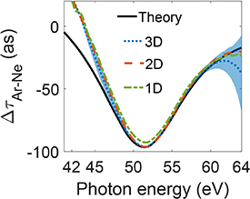
We have then applied the 3D approach to the calculation of the relative photoemission time delay, with the same pulse parameters used in section 3.2. The result is reported in figure 7. The relative photoemission time delay is reconstructed with good accuracy. With respect to the 2D simulations (green line in figure 7), an increase in the reconstruction convergence error is observed. This is a consequence of the IR CEP averaging, induced by Gouy phase variation over z, making it more challenging for the algorithm to define a unique IR temporal profile.
Figure 7. Reconstruction of photoemission time-delay obtained using the 3D, 2D and 1D approaches, assuming  and
and  W cm−2. The shaded area represents the standard deviation of the reconstruction, obtained by varying the initial guess for the IR temporal duration from 4 fs to 10 fs. Black solid curve shows
  calculated by using the atomic dipole phases reported in literature [33].
Download figure:
Standard image High-resolution image
5. Conclusions
We calculated the streaking traces produced by the interaction of an attosecond XUV pulse and an IR streaking pulse with an ensemble of atoms, taking into account the radial intensity distribution of the XUV and IR beams in a finite interaction region along the propagation axis. Ensemble effects notably affect the streaking traces, particularly upon decreasing the IR beam's spot size compared to that of the XUV beam and upon increasing the IR peak intensity. We showed that the reconstruction of the duration of the attosecond pulses and of the peak intensity of the streaking pulses are severely affected by ensemble averaging when the spot size of the IR beam is smaller than ∼2 times the XUV spot size. We proved that standard reconstruction techniques such as ePIE are capable of accessing spectroscopic information as the photo-ionization time delay if a parallel reconstruction exploiting two streaking traces sharing the same fields is used. The results reported in this work provide well-defined boundaries on the suitable experimental conditions that have to be used for both photoemission phase (time-delay) measurements and ultrashort pulse characterization, performed with the attosecond streaking technique.
Acknowledgments
This project has received funding from the European Research Council (ERC) under the European Union's Horizon 2020 research and innovation programme (Grant No. 848411—AuDACE, Grant No. 951224—TOMATTO), from MIUR PRIN aSTAR, Grant No. 2017RKWTMY, from MIUR PRIN, Grant No. 20173B72NB and from Fondazione Cariplo (Grant No. 2020-4380 DINAMO). We further acknowledge A Bresci and D Polli for sharing the computational nodes to run 3D simulations.
Data availability statement
The data that support the findings of this study are available upon reasonable request from the authors.
Conflict of interest
The authors declare no conflicts of interest.