

Abstract
Magnetic refrigeration is a highly active field of research. The recent studies in materials and methods for hydrogen liquefaction and innovative techniques based on multicaloric materials have significantly expanded the scope of the field. For this reason, the proper characterization of materials is now more crucial than ever. This makes it necessary to determine the magnetocaloric and other physical properties under various stimuli such as magnetic fields and mechanical loads. In this work, we present an overview of the characterization techniques established at the Dresden High Magnetic Field Laboratory in recent years, which specializes in using pulsed magnetic fields. The short duration of magnetic-field pulses, lasting only some ten milliseconds, simplifies the process of ensuring adiabatic conditions for the determination of temperature changes,  . The possibility to measure in the temperature range from 10 to 400 K allows us to study magnetocaloric materials for both room-temperature applications and gas liquefaction. With magnetic-field strengths of up to 50 T, almost every first-order material can be transformed completely. The high field-change rates allow us to observe dynamic effects of phase transitions driven by nucleation and growth as well. We discuss the experimental challenges and advantages of the investigation method using pulsed magnetic fields. We summarize examples for some of the most important material classes including Gd, Laves phases, La–Fe–Si, Mn–Fe–P–Si, Heusler alloys and Fe–Rh. Further, we present the recent developments in simultaneous measurements of temperature change, strain, and magnetization, and introduce a technique to characterize multicaloric materials under applied magnetic field and uniaxial load. We conclude by demonstrating how the use of pulsed fields opens the door to new magnetic-refrigeration principles based on multicalorics and the 'exploiting-hysteresis' approach.
Export citation and abstract BibTeX RIS

Original content from this work may be used under the terms of the Creative Commons Attribution 4.0 license. Any further distribution of this work must maintain attribution to the author(s) and the title of the work, journal citation and DOI.
1. Introduction
Magnetic cooling is a refrigeration technique that is based on the so-called magnetocaloric effect (MCE), the change of temperature caused by a magnetic field [1–5]. Its working principle is illustrated in figure 1. A paramagnetic material (left side of figure 1) being exposed to a magnetic field will partially align its magnetic moments along the external field and the magnetic entropy  is reduced. The total entropy, that has to be constant under isentropic (reversible adiabatic) conditions, is given by:

where the change in the entropy of the conduction electrons  is negligible for many magnetocaloric materials [6, 7] as well as any possible cross-coupling contributions [8, 9]. For this reason, the entropy of the lattice
  has to increase in order to keep the total entropy constant. As a result, the lattice vibrations are enhanced, which is the origin of the temperature increase when the material is being magnetized (right side of figure 1). Removing the magnetic field leads to the inverted effect and the material cools down again. By coupling the magnetocaloric material thermally with a heat-exchange fluid, for instance water, a cooling cycle consisting of four steps can be built [10].
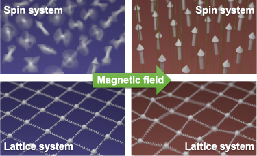
Figure 1. Explanation of the magnetocaloric effect. Starting from a paramagnetic material (left images), the application of a magnetic field leads to the partial alignment of the magnetic moments and the entropy of the spin system decreases. Under reversible adiabatic conditions, the total entropy is constant, which is why the lattice entropy has to increase. Phonons are created and, therefore, the material heats up.
Download figure:
Standard image High-resolution imageThe historical development of magnetocaloric research offers intriguing insights into the field. Figure 2 illustrates the number of publications in the field of magnetocalorics over the last decades. Until the year 2000, approximately 230 papers had been published and since then the total number has increased rapidly. Furthermore, on the right axis, the yearly publications are shown as bars. In 2014, for the first time, more than 500 new works were added to the literature. A closer look reveals that the number of publications began to increase drastically as early as 1990. Until today, the growth of knowledge continuous unabated [11–15].

Figure 2. Development of the total number of publications (left axis) in the field of magnetocalorics over the last decades. The right axis shows the normalized number of manuscripts that have been published each year (see text). The inset shows the normalized number of citations of the most-cited publications. The normalization was done by dividing the number of citations by the age of the paper. Data taken from Web of Science.
Download figure:
Standard image High-resolution imageIn order to identify the important scientific breakthroughs in magnetocalorics, the inset in figure 2 shows the normalized number of citations of the most-cited publications of each year. The normalization was done by dividing the number of citations by the age of the paper. Even if it looks inconspicuous, 1990 was a quite special year for magnetocalorics. Back then, Nikitin et al showed for the first time measurements of the adiabatic temperature change of Fe–Rh with a remarkable value of −12.9 K in only 1.95 T field change [16]. The impressive magnetocaloric performance of this material was predicted theoretically by Ponomarev already in 1972 [17], even though this and other works of this group [18] are almost unknown.
The peak in 1993 originates in the paper form Sessoli et al in Nature with the title 'Magnetic bistability in a metal-ion cluster' having more than 3500 citations [19]. This is a good example showing that the field of magnetocalorics is very broad. In that paper, the magnetic properties of metal-ion clusters below 10 K are studied. Although this particular work may not have direct implications for room-temperature cooling applications, it nonetheless serves to underscore the presence of the MCE in every magnetic material, particularly in the vicinity of magnetic phase transitions [20]. In any case, the field of magnetic cooling got a tremendous boost during that period, which fortunately was followed by a consolidation of our research area in 1997 with the discovery of the so-called giant MCE in Gd5(Si,Ge)4 by Pecharsky and Gschneidner [21]. This breakthrough had a profound impact on the field, greatly expanding the potential for magnetic cooling technologies and the latter paper is, until today, the most-cited paper in magnetocaloric's history.
In addition to the aforementioned publications, individual breakthroughs, such as the discovery of the giant MCE at room temperature in Mn–Fe–P–As by Tegus et al in 2002 [22], the exploration of the inverse MCE in Ni–Mn–Sn alloys in 2005 by Krenke et al [23], and the exploitation of multicaloric effects in Heusler materials by Liu et al in 2012 [4], are visible in this plot (inset of figure 2) as they lead to the peaks at these specific years. It is particularly noteworthy that review papers on the state of the art of magnetocalorics are frequently cited. These papers appear regularly at intervals of about 3–4 years, for example in 2007 [24], 2011 [25], 2014 [26], and 2018 [1].
While all these articles show, that it is common to use indirect methods to study caloric materials, since determining temperature changes under adiabatic conditions can be experimentally very challenging [27], it is ultimately desirable to measure the caloric response  directly [26, 28]. Of the total of 8500 publications on magnetocalorics, we estimate that less than
  address the topic of adiabatic temperature changes at all, and an even smaller proportion presents actual and direct measurements.
On the basis of this premise, the technique of the direct determination of the adiabatic temperature change,  , in pulsed magnetic fields has been developed in recent years at the Dresden High Magnetic Field Laboratory (HLD) [29, 30] and in other labs, for instance see [31–37]. The schematic in figure 3 illustrates the measurement capabilities that pulsed magnetic fields can offer in terms of the characterization of magnetocaloric materials. An appropriately designed tandem of capacitor and solenoid can generate high magnetic fields in very short time scales.

Figure 3. By using a large capacitor bank and non-destructive solenoids, we can produce magnetic field pulses of up to 95 T. On the right, a typical time dependence of a pulsed field is shown.
Download figure:
Standard image High-resolution imagePulsed fields have several advantages when it comes to the characterization of magnetocaloric materials. First, the short duration of the field pulses of only a few milliseconds makes it relatively straightforward to ensure adiabatic conditions and enables to study dynamic effects of phase transitions that are driven by nucleation and growth processes. Second, the magnetic-field strength is sufficiently high to transform almost every material with a first-order phase transition completely, which is important in order to learn about the maximum possible temperature change. However, accurately measuring temperature changes within such a short time frame is a challenging task and requires dedicated hardware. In this paper, we aim to provide a comprehensive overview of the beauty and diversity of our methods exemplifying results for different magnetocaloric materials.
2. Experimental details
Given the specialized nature of our methodology and the unique infrastructure required, this section will give a more extensive explanation of the experimental set-ups and the associated individual challenges that are encountered.
The MCE is directly measured at the Dresden High Magnetic Field Laboratory (HLD), Member of the European Magnetic Field Laboratory (EMFL), Helmholtz-Zentrum Dresden-Rossendorf (HZDR), utilizing pulsed magnetic fields produced by in-house-developed non-destructive solenoids that are capable of generating high magnetic fields up to 95 T [38, 39]. In the experiments described in the following, the so-called KS11 coil was used to produce magnetic fields of up to 50 T as depicted in figure 4, with change rates of the field shown in the inset of the plot. The field rapidly reaches its maximum value within the first 13 ms, as indicated by the  value, before decreasing to zero, with each pulse lasting a total of about 100 ms. The amplitude of the field can be varied by adjusting the voltage applied to the coil, while the duration of the pulse and the shape of the field change exhibits a reproducible behavior determined by the design of the coil and capacitor bank. At the Dresden High Magnetic Field Laboratory, we have magnets that can produce pulses between about 25 ms and 1.5 s. However, short-pulse magnets are not adequate for this specific technique as the experimental challenges increase considerable, as we will discuss later. The magnet is placed in a vessel with liquid nitrogen. After each pulse, the magnet needs to cool down, so the number of pulses is limited in time. For instance, the repetition time for a 10 T pulse is around 15 min, while almost 2 h are needed after a 50 T pulse.

Figure 4. Typical time-dependent magnetic field for different field strengths in the pulse-field coil KS11 at the Dresden High Magnetic Field Laboratory (left scale). For each pulse, the maximum is reached after  and depends on the applied voltage to the coil. The violet curve represents the voltage induced in the pick-up coil during the pulse that is integrated to extract the magnetic field (right scale). The inset shows the time derivative of the magnetic field as a function of field itself. It is noteworthy that the field profile is invariant with respect to its shape.
Download figure:
Standard image High-resolution imageIn this section, we outline the experimental technique with a focus on the utilization of thermocouples. Additionally, we address the most common experimental challenges encountered in pulse-field experiments.
2.1. Experimental set-up
Figure 5 shows a schematic drawing of the pulse-field experimental set-up. The experiment comprises a bath cryostat with a long tail, which is placed in the center of the coil. The use of liquid helium enables to attain cryogenic temperatures as low as 4.2 K. A sample insert, constructed in-house, is mounted within the cryostat. The sample holder (figure 5(c)) is made out of polyether ether ketone, a semicrystalline thermoplastic with excellent mechanical properties, chemical resistance, and low thermal conductivity. The sample is secured in place using a small amount of GE Varnish. A local heater, consisting of a manganine wire wrapped around a thin brass cylinder, is placed around the sample to control its temperature. The double pick-up coil measures the field change in the center of the sample holder. Only a few turns of wire are sufficient for a reasonable measurement as the field-induced voltage in the pick-up coil is quite large (see right scale of figure 4). A differential thermocouple made from thin, 25 µm thick, wires is used to determine the temperature of the sample. The measuring end of the thermocouple is bonded between two flat, polished sample pieces with a small amount of heat-conducting silver epoxy. The second reference junction is attached to the thermometer on the back side of the holder (figure 5(c)). A more in-depth explanation on the temperature determination is provided below. The sample insert is housed within a stainless-steel vacuum tube, which is evacuated to a pressure of  mbar in order to prevent heat exchange between the sample and the surrounding environment on the time scale of the pulse. The heater and thermometer are connected to a LakeShore 350 temperature controller, figure 5(b). The thermocouple and double pick-up coil are connected to an oscilloscope recording signals in 2 µs steps. This experimental set-up allows to connect additional sensors for simultaneous measurements or to use several thermocouples.

Figure 5. Experimental set-up for direct pulse-field measurements of the adiabatic temperature change. (a) The schematic representation shows the pulse-field coil placed in a tank with liquid nitrogen. The cryostat is installed in the bore of the coil. The insert with the sample is mounted inside a vacuum tube. (b) Temperature sensor and heater are connected to a LakeShore 350 temperature controller. An oscilloscope is synchronized with the magnet power supply and reads the pick-up coil and thermocouple signals. (c) The plastic sample holder with two pick-up coils, cylindrical heater, thermometer, thermocouple, and the sample. The reference thermocouple junction is placed near the thermometer. The second end is glued between two polished sample pieces, as it is illustrated in (d). The red circle shows a zoomed image of the thermocouple junction. The used wire thickness is 25 µm.
Download figure:
Standard image High-resolution image2.2. Temperature measurement using thermocouples
A differential thermocouple is a device that utilizes the Seebeck effect to measure temperature differences by detecting the electromotive force generated across two junctions of dissimilar metals [41]. For example, if both junctions of the thermocouple are at the same temperature, the resulting thermal-voltage output is zero regardless of the temperature gradient within the wires connecting the junctions. For a non-zero temperature difference, the voltage depends on both junction temperatures. By measuring both the temperature of the reference junction with a thermometer and the thermal voltage of the entire thermocouple, we can determine the temperature of the junction attached to the sample using a calibration curve.
The thermocouple junctions are positioned on the sample holder to ensure minimal temperature gradients between them prior to applying the magnetic field. This configuration improves the precision of the measurements.
In addition, this also allows for a shorter length of the thermocouple and, therefore, a smaller electrical resistance. This is important, because even with the small electrical capacitance between the twisted-pair wires, the RC time constant can become significant when the wire resistance is large, leading to a time delay in the transient process in the circuit.
We prepare thermocouples of wires with a diameter of only 25 µm in order to reduce their thermal mass. Depending on the temperature range, we use one of two thermocouple types: a combination of copper and constantan (type-T) for near-room-temperature measurements, or constantan and chromel wires (type-E) at cryogenic temperatures. Figure 6(a) shows the calibration of both thermocouple types done in our laboratory, which agrees well with the NIST database [40]. To detect parasitic effects caused by the magnetic field, we also tested both types of thermocouples without samples in pulsed fields at different initial temperatures, see figure 6(b). The measured signals were filtered and converted to temperature. Regardless of the field strength, the resulting temperature signals demonstrated no sensitivity to the magnetic field. At the same time, the noise level increased as thermocouple sensitivity decreased towards low temperature. Consequently, it is preferable to use type-E thermocouples in cryogenic experiments.

Figure 6. (a) Calibration curves of the measured voltage of thermocouples as a function of temperature, normalized to 273.15 K. Data taken from [40]. (b) Noise in E- and T-type thermocouples, getting more noticeable at lower temperatures. (c) Schematic of the measurement of the temperature difference realized in an experiment. (d) Schematic of the thermal voltage and temperature difference as a function of time.
Download figure:
Standard image High-resolution imageFigures 6(c) and (d) schematically show the procedure for converting the measured signal into temperature. As stated above, the reference end of the thermocouple is located in close proximity to the sample and the temperature  is determined with a thermometer. Using the functions
  , we determine the corresponding reference voltage
  with respect to 0 ∘C. The measured thermocouple signal
  is filtered to remove noise, and is then added to the value of
  . Subsequently, the inverse transformation
  is applied to obtain the sample temperature throughout the duration of the experiment,
  .
.
2.3. Experimental challenges
Direct measurements of the MCE with the method described above carry some experimental hurdles to be considered and overcome. These are mainly due to the very small time window of the measurement and the very fast field changes. The major challenges are described here as follows.
2.3.1. Eddy-current heating
The most obvious challenge in conducting temperature measurements in the presence of alternating magnetic fields is the potential for eddy-current heating. Despite the magnetic-field changes, heating of the samples due to eddy currents is not observed in our experiments. Joule heating is proportional to the square of the current density induced in a conductive sample by a changing magnetic field [42], therefore, the temperature of the sample should rise throughout the entire pulse. In our experiments, the absence of this effect is confirmed by the fact that the temperature before the field application is equal to the temperature at the end of the pulse in the case of a fully reversible MCE as, for instance, in second-order materials. Additionally, in cases where the MCE is zero, such as when being far away from the transition temperature, we also observe no field-induced temperature change.
2.3.2. Delayed thermal response
One of the issues sometimes encountered is the insufficient thermal coupling between the sample and the thermocouple. This is illustrated in figure 7, which shows a typical MCE for a second-order magnetic-transition material near its Curie point. The MCE induced by a field change shows no magnetic hysteresis in these materials. Nevertheless, a hysteresis might be detected during the measurement (see figure 7). This can be attributed to a delayed response of the temperature measurement compared to the true sample temperature.
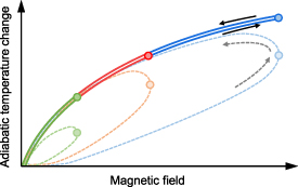
Figure 7. Schematic example of the adiabatic temperature change as a function of magnetic field for a second-order material near its Curie temperature (solid curves). Black arrows indicate up- and down-sweep trajectories, there is no thermal hysteresis. Dashed lines and arrows show the influence of a thermal delay on  for different pulse strengths.
Download figure:
Standard image High-resolution imageFor instance, a delay might occur when too much adhesive is placed between the thermocouple junction and the sample or when the thermal contact is weak. The time delay of the temperature measurement, thus, leads to a distortion of the measured effect in relation to the field. Therefore, the maximum of the MCE is not reached at the maximum of the applied field, but only when the field is already in the down sweep and the real temperature of the sample is cooling down. This leads to an underestimation of the MCE. Furthermore, different maximum field strengths and, consequently, different field-change rates lead to delay effects. Such delay is most critical for first-order magnetic-transition materials, where intrinsic hysteresis overlaps with the delay hysteresis and it is impossible to separate them. To keep the delay as small as possible, it is necessary to use only a little amount of silver epoxy, and mount the thermocouple connection preferable in a 'sandwich' of two pieces of the sample. In this way, a large area of the thermocouple is in contact to the sample. Alternatively, the thermocouple can also be welded to the sample or be prepared by sputtering.
2.3.3. Magnetic-field induced signal
According to Faraday's law, if a wire loop area with the vector  as a parallel component to an applied field
  , an electromotive force is induced by a time-varying magnetic field [43]:

This leads to strong parasitic signals in pulse-field measurements due to the high field-change rates. As seen for the pick-up signal in figure 4, the induced voltage is in the order of several volts for a pick-up coil with only a few turns. To avoid such signal, it is of great importance to twist the thermocouple wires tightly to minimize open loops in the wire circuit. Other potential sources of interference that are not located inside the magnet have a limited impact on the measurement, because already at a distance of 15 cm from the center of the solenoid, the field strength is reduced to about  [39].
[39].
Despite the presence of an electromotive force, it is still possible to extract a useful thermocouple signal. One approach is to utilize the voltage from the field-pick-up coil, as this signal is similar in shape to the parasitic signal produced by loops in the thermocouple (figure 4(a)). Therefore, it can be utilized for correction with an appropriate proportionality factor. However, this alone may not be sufficient in every case.
An alternative approach for correction is to take advantage of the fact that the induced signal depends on the direction of the magnetic field relative to the loop. By applying two pulses of the same amplitude in opposite directions, the parasitic electromotive force has the same amplitude, but with negative sign. Instead, the value of the MCE does not depend on the sign of the field. Taking the average of a positive and negative field pulse will, therefore, cancel out the parasitic signal. Figure 8 illustrates the adiabatic temperature change  with respect to time for two distinct pulses, one with positive field direction (a) and the other with negative field direction (b). Figures 8(c) and (d) show the average signal obtained by combining both pulses, in which the parasitic signals are mutually cancelled as a function of time and magnetic field, respectively. This method requires more pulses and, therefore, increases the time required for the measurement. However, we demonstrated that performing the procedure at a limited number of initial temperatures and interpolating the results for intermediate temperatures is sufficient to achieve accurate results. Usually, it is adequate to carry out this approach for one field amplitude (e.g. 10 T) and apply the appropriate scaling factor for other field strengths.

Figure 8. Time dependence of thermocouple signals. The induced parasitic electromotive force, which is proportional to  , depends on the field direction. It contributes to the thermocouple signal differently in (a) positive and (b) negative field pulses. The averaged signal contains no induced signal, neither over time (c) nor over field (d).
Download figure:
Standard image High-resolution image3.
 characterization of magnetocaloric materials

To characterize the adiabatic temperature change of materials in pulsed magnetic fields, we measure at selected temperatures covering the range around their magnetic transitions. From each measurement,  at a specific maximum field value is extracted and, consequently,
  for different initial temperatures is obtained. Even though the pulse-field magnets at the HLD can ramp up to 50 T (or higher), it is common to determine the MCE of a material at smaller field values starting from 2 T.
Before a high-field experiment, it is useful to know the magnetic properties of the samples in static fields in order to determine parameters such as transition temperatures, order of the transition (second or first order), the sensitivity of the transition to the field ( ). This allows to define a measurement protocol. For second-order materials, such as Gd, no special care is required since there is no thermal hysteresis involved. The measurement may be performed by constantly heating and cooling the specimen over a wide temperature range, illustrated in figure 9(a) using sufficiently low ramp rates in order to avoid temperature gradients within the sample. Typical heating and cooling rates are of the order of 0.2 K min−1 or less. The magnetic field is applied and removed in certain temperature intervals. It is to be considered that the magnetic-field application is fast enough in comparison to the utilized heating/cooling rate to avoid metrological errors. Alternatively, the sample temperature can be stabilized at each measurement point as depicted in figure 9(b).
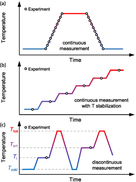
Figure 9. Schematic illustration of (a) a continuous protocol, (b) a continuous protocol with temperature stabilization and (c) a discontinuous measurement sequence.
Download figure:
Standard image High-resolution imageWhen the material under investigation shows a large thermal hysteresis, the  measurements need to be unaffected by previous field applications and under conditions that allow the determination of the reversible effect. Due to the thermal hysteresis, the results will depend on the measurement protocol chosen to reach the initial temperature
  ([44] and references therein). One facet is that the effect becomes irreversible at temperatures inside the hysteresis area. The discontinuous protocol as depicted in figure 9(c) is applied here in order to erase the memory of the material. In general, a second field application delivers reliable results of the reversible
  [45, 46].
As an example, we show results for the Heusler alloy Ni45Co5Mn38Sb12 [44]. Figure 10 provides  results for 6 T pulses, where
  was reached following discontinuous heating and discontinuous cooling protocols (see figure 9(c)) as well as a continuous heating protocol (see figure 9(b)). In the first two experimental runs, the sample was always heated up to the high-temperature phase (around 300 K) and cooled down to the low-temperature phase (100 K, or vice versa) before reaching the initial temperature
  . In the case of continuous heating,
  was just approached by heating directly from the previously measured temperature. There is a huge difference in the
  obtained depending on the protocol. The curves are not only shifted in temperature, as expected, but the maximum
  differs strongly as well. This deviation follows the thermal hysteresis observed in the M(T) curves (see inset of figure 10).

Figure 10. Adiabatic temperature change of Ni45Co5Mn38Sb12 around the martensitic transformation, obtained with 6 T pulses following discontinuous heating (red symbols), discontinuous cooling (blue symbols) and continuous heating (open red symbols). The inset shows temperature-dependent magnetization curves recorded in 0.01 T during cooling and heating. The temperatures at which  was recorded are highlighted. Data taken from [44].
Download figure:
Standard image High-resolution imageThe application of a magnetic field only induces the transition from the low- into the high-temperature phase as it favors the phase with the larger magnetic moment. Consequently, the transformation can only occur at temperatures where some low-temperature phase is present in the sample before the pulse (below the martensitic start temperature  K). Upon discontinuous heating protocol, the first-order transition (FOT) takes place below the austenitic finish temperature
  K. We also performed measurements following the continuous heating protocol. The
  values obtained using this method are lower than the ones obtained under discontinuous heating as the previous field application induces partially, or completely, a transition to the high-temperature austenite and some of the phase is retained after field removal [47]. This arrested austenite (not present in the case of discontinuous heating) does not contribute to the cooling effect and acts as a heat load. In other words, each
  measurement depends on the previous ones [48]. Therefore, results obtained in this way are, in general, difficult to interpret and not reproducible.
The following subsections give an overview of the standard characterization in pulsed magnetic fields of the three different types of transitions one might encounter in magnetocaloric materials, namely the conventional second-order, conventional first-order, and the inverse first-order transformation [49].
3.1. Materials with second-order phase transition
Materials that undergo a second-order phase transition exhibit a conventional MCE, that is a warming under magnetic-field application [1]. This is, for instance, the case for a magnetic transition between a para- and a ferromagnetic phase around the Curie temperature  . Some example materials studied in pulsed magnetic fields, are the rare-earth element Gd [50], Laves phases [51], Mn5Ge3 [52], and GdNi2 [53]. We discuss the case of Gd and the Laves-phase compound HoAl2 in detail below.
3.1.1. Gadolinium
The adiabatic temperature change of a Gd single crystal was measured in high magnetic fields up to 62 T [50, 54]. The field dependence of  for selected initial temperatures is plotted in figure 11(a). As can be seen, even up to the highest fields, the effect is reversible without the emergence of a metrological hysteresis due to a thermal delay or eddy currents as discussed in section 2.3. The maximum
  at different fields is plotted in figure 11(b) as a function of the initial temperature. We observed a pronounced maximum of 60.5 K around 300 K and no sign of saturation is present. Contrary to the conventional picture that the largest MCE always appears at the Curie temperature (294 K for Gd) and scales with
  , we could demonstrate that the position of the maximum is shifting towards higher temperature with increasing field. On the basis of the experimental findings, we developed a mean-field model being in perfect agreement with the measurements suggesting that terms of higher order gain importance in fields above
  (see [50] for more details). Furthermore, from the
  values, it is also possible to determine the isothermal entropy change
  at high fields. Figure 11(c) shows the entropy difference related to a reference
  without magnetic field calculated from zero-field specific-heat data. The entropy curves at a given magnetic fields can be generated from this using the
  data. In this way,
  for fields up to 62 T is obtained for Gd and plotted in figure 11(b). It is worth noting that there is no other way of obtaining
  for such high fields experimentally.

Figure 11. (a) Field-dependent  at selected temperatures for a Gd single crystal up to 62 T. (b) Maximum
  as function of initial temperature
  together with calculated
  curves. (c) Entropy difference in zero field, calculated from specific-heat data and calculated entropies for 20 and 62 T. The black arrow illustrates the extraction of
  from
from  values (red arrow). Data taken from [50].
Download figure:
Standard image High-resolution image3.1.2. Laves phases
The second example covers a completely different temperature range as in the previous example. Laves phases are promising materials for gas liquefaction based on the MCE [51, 55–57]. Therefore, measurements down to low temperatures are necessary to study these materials. It is worth noting that the characterization of materials below 100 K involves extra experimental challenges, such as the requirement of liquid helium to reach cryogenic temperatures. In some cases, the use of type-E thermocouples is needed to gain sensitivity as mentioned in the experimental section. Our example, HoAl2, undergoes a second-order phase transition at  K [51]. We characterized the MCE in this material in pulsed magnetic fields up to 50 T in a temperature range between 20 and 120 K. Figure 12 presents the maximum
  as a function of initial temperature for different magnetic-field changes. The inset shows the temperature change of the sample as a function of field obtained for
  K for a field pulse of 50 T. From these results, the values at different field changes are extracted, as indicated in the figure. Other than in the case of Gd, the maxima of the
  curves are located in close proximity to
  . A field change of 50 T is, therefore, not high enough to see the influence of higher-order terms. For 10 T, the adiabatic temperature change calculated from specific-heat measurements is also plotted in figure 12 with excellent agreement between both techniques.

Figure 12.
 measured up to 50 T for HoAl2 as function of initial temperature
  . Values calculated from specific-heat data (lines) are shown for 10 T. The inset shows the temperature change as function of applied field for 2, 10, 20, and 50 T pulses starting at
  K. Data taken from [51].
Download figure:
Standard image High-resolution image3.2. FOT with conventional MCE
The second important class of magnetocaloric materials are the ones which exhibit an FOT with conventional MCE. Typically, the material is ferromagnetic at low temperatures. At  , the material transforms into a high-temperature phase with low magnetization due to a first-order magnetostructural or magnetoelastic transition [49]. An applied magnetic field shifts the transition toward higher temperatures. At temperatures above
  , an FOT from the paramagnetic to the ferromagnetic phase can be induced by applying an external magnetic field. Thermal hysteresis is always involved in the FOT, therefore, the discontinuous cooling protocol is usually followed. From this class of materials, we have characterized La–Fe–Si [58], Mn–Fe–P–Si [59], Ni–Mn–Ga [60, 61], and others in pulsed magnetic fields. We present the examples La–Fe–Si and Mn–Fe–P–Si in detail below.
3.2.1. La–Fe–Si
The first example for this class of materials is LaFe11.74Co0.13Si1.13 with  K. Details of the material can be found in [58]. Figure 13(a) shows the maximum
  values as a function of
  obtained for field changes of 2, 5, 10.5, and 50 T. For 2 T,
  shows a sharp maximum around
  . When increasing the magnetic field, the observed peak broadens asymmetrically towards higher temperatures. One main difference compared to second-order materials is the sharp edge on the low-temperature side of the curves. This can be explained as follows: at temperatures below
  , the sample is in the ferromagnetic state and applying a magnetic field only marginally changes the magnetic entropy of the system and, thus, also
  . Above
  , an applied magnetic field can induce the transition resulting in two contributions to the MCE, the conventional behavior of the alignment of magnetic moments in the paramagnetic phase and the contribution of the FOT. The peak broadens towards higher temperatures as far as the applied field is sufficient to induced the transition. In this specific case, 5 T is strong enough to transform the material completely at least in the temperature window between 195 and 205 K as indicated by the plateau in figure 13(a).

Figure 13. (a)  as a function of
  for 2, 5, 10.5, and 50 T pulses for La–Fe–Co–Si. (b) Isothermal magnetization at selected temperatures obtained in static fields (in color) and magnetization obtained at
  K in pulsed fields (dashed black). The inset shows field-dependent
  data at 188 and 212 K for 10 T pulses. Data taken from [58].
Download figure:
Standard image High-resolution imageAt higher fields, we observe no saturation of the temperature change, which is due to the strong influence of the paramagnetic phase. The interplay of first- and second-order contributions are also evident in the inset of figure 13(b). This diagram shows  as a function of field for
  and 212 K for 10 T pulses. As
  , the MCE originates in an additional alignment of spins in the ferromagnetic phase and resembles a conventional second-order effect. However at 212 K, a transition from the para- to the ferromagnetic phase is induced with field and the
  curve shows a hysteresis between up and down sweep indicating the first-order character of the transition (inset of figure 13(b)).
Figure 13(b) shows isothermal magnetization curves measured in static fields. The field-induced transition is clearly seen as a sharp change in magnetization. Additionally, an adiabatic curve obtained in a pulse-field experiment at the initial temperature  K is also included. There is a large difference between the quasi-static and pulsed-field results, because of the simultaneous heating effect of more than 13 K in pulsed fields. For this reason, the adiabatic magnetization curve intersects the corresponding isotherms. This is an important finding because, whenever a material with a magnetic transition is examined in pulsed fields, a significant MCE can also occur and, thus, the magnetization curve is influenced.
3.2.2. Mn–Fe–P–Si
Another material example that exhibits an FOT with conventional MCE is Mn–Fe–P–Si. Here, we show results for a sample with a similar composition as the one published in [59]. This compound has a hexagonal lattice and undergoes an isostructural phase transformation from a ferromagnetic to a paramagnetic state at around 260 K. The application of magnetic field shifts the transition towards higher temperatures as can be seen in the inset of figure 14(b), where we plot different temperature-dependent magnetization curves. We characterized the MCE around the transition with 2, 5, 10, 20, and 50 T pulses. For all measurements, a discontinuous cooling protocol was followed to reach  . The maximum values of
  are plotted in figure 14(a). There is no saturation of
  even up to 50 T. As mentioned before, this is related to the conventional second-order MCE of both the para- and ferromagnetic phase that overlaps with the MCE caused by the FOT.

Figure 14. (a)  as a function of
  for 2, 5, 10, 20, and 50 T pulses for Mn–Fe–P–Si. (b) Field-dependent
  data at 260 K for different fields. The arrows indicate the field-sweep directions. The inset shows magnetization at different fields obtained in static fields upon cooling.
Download figure:
Standard image High-resolution imageFigure 14(b) shows field-dependent  results obtained at
  with field changes of 2, 5, 10, 20 and 50 T. At this temperature, the field application induces the first-order ferromagnetic transition and the temperature of the materials increases. The curves for field application do not overlap with the ones for field removal. This field hysteresis of the
  curves results from the thermal hysteresis of the FOT. On the other hand, as was discussed before in figure 5, all magnetic-field pulses reach their maximum after 13 ms resulting in field-sweep rates ranging from 0.2 to 10 kT s−1. The slopes of the increasing-field curves depend on the sweep rate, while the slopes for the down sweeps, where the field-change rates are considerably smaller, are similar. This led us to the conclusion that, on the one hand, a certain delay in the thermocouple might play a role especially for highest fields, but, on the other hand, also dynamic effects of the first-order phase transition are involved. The nucleation and growth of the ferromagnetic hexagonal phase formation lacks behind the magnetic field change (see [59] for more details). Additionally, as 260 K lies in the middle of the thermal hysteresis being an intrinsic feature of the FOT, the MCE effect is partly irreversible and, therefore, the temperature of the sample after the pulse is higher than before.
3.3. FOT with inverse MCE
In materials of this group, also a first-order magnetostructural phase transition is taking place. However, the low-temperature phase has a lower magnetization than the high-temperature one. Therefore, a magnetic field shifts the transition to lower temperatures and  is negative [49]. The transition can be induced by magnetic field at temperatures below
  and the material cools under field application resulting in an inverse MCE. Another main difference with the former group of materials is that
  reaches saturation at certain magnetic field [49]. The Ni–Mn-based Heusler alloys [30, 44, 62–65], Mn3GaC [29], FeRh [66–68], among others belong to that group. In the following, we discuss examples of the Ni–Cr–Mn–In Heusler alloy and Fe–Ni–Rh.
3.3.1. Heusler alloys
A well-studied case are the magnetic Heusler alloys, where a first-order martensitic magnetostructural transition takes place between two magnetic phases. We show the example of the Heusler alloy Ni50Cr2.5Mn32.5In15.0 in figure 15 [63]. Upon cooling, this material undergoes a first-order martensitic transition at around 270 K from a high-temperature ferromagnetic austenite to a low-temperature martensitic phase, which exhibits a lower magnetic moment. Upon heating, the martensite-to-austenite transition takes place at around 280 K (see inset of figure 15), so there is a significant hysteresis present. Around  , the material has a conventional MCE and in the vicinity of the martensitic transition, the MCE is inverse as can be seen in figure 15(a), showing the adiabatic temperature changes as a function of the starting temperature
  for 2 and 6 T pulses.
  was reached following the discontinuous heating protocol (closed symbols). At selected temperatures inside the hysteretic region, we performed a follow-up pulse (open symbols) to study the reversibility of the effect as discussed previously.

Figure 15. (a)  as a function of
  for 2 and 6 T pulses for Ni50Cr2.5Mn32.5In15.0. The discontinuous heating protocol was used to reach
  , except for the results plotted with open symbols which were obtained upon a 2nd field application. The inset shows magnetization data at 0.01, 2 and 6 T fields obtained in static fields upon heating and cooling (see arrows). (b) Field-dependent
  data at selected temperatures obtained for 6 T pulses. The green curve shows the second application of the pulsed magnetic field at 275 K. Data taken from [63].
Download figure:
Standard image High-resolution imageFigure 15(b) shows field-dependent data of  at selected temperatures for 6 T pulses. At
  , we observed a conventional MCE, the sample temperature increased with field. At
  and 275 K, an inverse MCE leads to a decrease of the sample temperature with increasing field. Furthermore, the shape of the field-dependent
  is completely different in comparison to the results previously shown for other materials showing a large magnetic hysteresis.
Specifically, looking at the curve obtained at  (see figure 15(b)), the sample temperature does not change until the field reaches approximately 4.5 T, when the transition from martensite to austenite is induced. Only then, the sample cools down by about 4 K until the field reaches its maximum of 6 T. For the down sweep (the arrows indicate the field-sweep direction), first the sample shows a conventional magnetocaloric behavior in the induced ferromagnetic austenite i.e. the sample cools down further. When the field reaches about 3.8 T, the reverse transition from austenite to martensite takes place and the sample recovers its initial temperature. It is worth to mention that here the field was not sufficient to induce a complete transition as no saturation is observed at maximum field. At
  , lower field values are needed to induce the transition and the temperature of the sample starts decreasing already at around 1.5 T. The maximum obtained
  is around −7 K when the field reaches its maximum. This field is sufficient to complete the transition at this temperature, however, the hysteresis is larger and the reverse transition takes place when the field decreases to around 1.5 T. Furthermore, the MCE is highly irreversible due to the fact of being in the middle of the hysteretic region. After field application, a large fraction of the sample remains in the austenite and does not transform back to the martensite phase when the field is removed (the final temperature of the sample is lower than the initial
  ). When a second pulse is given (see green curve in figure 15(b)), the result is a mixture of inverse MCE, due to the transformation from martensite to austenite, and conventional MCE, caused by the austenite already present in the sample after the first pulse. As a consequence, the maximum obtained
  K is lower than that obtained for the first pulse. In general, this is the case for temperatures close and within the hysteretic region. The second field application gives more reliable results on the reversible effect. Data taken upon first field application tend to overestimate the MCE under cyclic operation [45, 46].
3.3.2. Fe–Rh
Our second example, (Fe0.98Ni0.02)49Rh51, we characterized in pulsed fields up to 14 T [66]. This material undergoes a first-order antiferro-ferromagnetic transition at 266.5 K in zero-field (on heating), which involves a volume change of about 1% without changing its crystal symmetry [69]. Applied magnetic field shifts the transition toward lower temperatures with a rate of −11 K T−1.
The temperature dependence of  obtained using the discontinuous mode upon first field application is plotted in figure 16(a) for 2, 5, 10, and 14 T pulses. Field-dependent
  data at selected temperatures are shown in figure 16(c). For instance, at 238 K (green curve), it is possible to see that the material starts cooling at around 2.5 T when the antiferro- to ferromagnetic transition is induced. At this temperature, the transition is completed when the field reaches 7 T and
  reaches a saturation value of −7 K (contrary to the results for Ni–Cr–Mn–In presented in figure 15(b) where saturation is not observed) and does not increase further with field. When the magnetic field is removed (the arrows indicate the direction), there is no change in the temperature until the reverse transition takes place, around 2 T. This magnetic hysteresis originates from the first-order character of the transition. As the temperature of measurement decreases, larger magnetic field values are needed in order to induce the transition. However, for 14 T pulses, a full transformation from the antiferromagnetic to the ferromagnetic phase is induced for all temperatures. The maximum
  decreases as the temperature of the pulse decreases as can be seen in figure 16(a). Specifically, at 122 K the maximum
  achieved is −2.5 K for a 14 T pulse.

Figure 16. (a)  as a function of
  for 2, 5, 10 and 14 T pulses for (Fe0.98Ni0.02)49Rh51. (b) Field-dependent magnetization measured under isothermal conditions in static fields at 201, 205, and 209 K and adiabatic conditions in pulsed fields at
  . (c) Field-dependent
  data at selected temperatures obtained for 14 T pulses. Data taken from [66].
Download figure:
Standard image High-resolution imageWe performed magnetization measurements under isothermal (static fields) and adiabatic conditions (pulsed fields) to study the dynamics of the FOT. Selected results around 205 K are presented in figure 16(b). In pulsed fields, the hysteresis loop is broader and has an asymmetric shape. One possible explanation for this is that the structural changes during the transition cannot follow the fast changes in pulsed fields, as we have discussed previously for Mn–Fe–P–Si. On the other hand, the induced transition is shifted toward higher fields due to the MCE. However, for the case of Fe–Rh it is not straightforward to relate the isothermal and the adiabatic magnetization results as in the La–Fe–Si–Co example. This motivates the need of simultaneous measurements of  , magnetization, and strain to fully understand the behavior of materials in pulsed magnetic fields.
4. Simultaneous measurements of physical properties
In the previous section, we concluded that to fully understand the magnetocaloric behavior of materials in pulsed magnetic fields, we need to measure different physical properties simultaneously. For instance, in the case of FOTs, where the results suggest that the structural transitions cannot follow the faster field changes [29, 30, 59, 66], measuring the strain gives a better understanding of the relation between structural and temperature changes in the sample. On the other hand, we also show that magnetization measurements in pulsed fields are not isothermal for magnetic materials. For this reason, we have developed the option to measure the magnetization simultaneously with the adiabatic temperature change and strain allowing the direct comparison of these properties and the exact determination of the phase diagram of a material, i.e. the critical fields of the transitions. The technique is illustrated schematically in figure 17, where (a) shows the strain gauge used to determine the relative changes in the sample length and the circuit to measure it, (b) shows a picture of the coil for magnetization measurements, and (c) sketches how the three experiments are mounted together. We describe the different methods in the following, based on the results obtained in a Fe–Rh sample at  for a 26 T pulse. Moreover, we present below the results on the simultaneous measurements of
  and length change in Ni–Mn–In and
  as well as magnetization in a Ni–Co–Mn–Ti sample.

Figure 17. (a) Circuit and principle to measure the resistance of strain gauges in pulsed fields. (b) Picture of the sample holder with the compensated split-coil magnetometer. (c) Schematic of the techniques for the simultaneous determination of  , length change, and magnetization.
Download figure:
Standard image High-resolution image4.1. Length change
Our method of choice for measuring length changes are strain gauges, devices whose electrical resistance changes proportionally to the strain of the device as indicated in the schematic of figure 17(a). A metallic strain gauge can consist of either thin wire or a metallic foil arranged in a grid pattern. The grid pattern maximizes the amount of metallic wire or foil subject to strain in the parallel direction. It also minimizes the cross sectional area of the grid to reduce the effect of shear strain and Poisson strain [70]. The strain gauge is carefully glued to one of the sample surfaces as illustrated in figure 17(c).
We measure the resistance changes of the strain gauge using a four-point method [71] or, alternatively, the Wheatstone-bridge technique [72]. In the case of the four-point technique, a frequency generator supplies an alternating excitation current to the strain gauge via a series resistor ( , as indicated in the schematic of figure 17(a)). The current flowing through the strain gauge is measured as a voltage across
  (
( ). Simultaneously, the voltage signal of the strain gauge (
 ) is recorded with the oscilloscope. The evaluation is done by a software that performs a digital lock-in calculation [73], as follows. First, from
  , the frequency (
 ) and phase (
 ) of the excitation signal are determined and a sine function with this parameters is created. Then, both
  and
and  are multiplied by this sine wave. A band-pass filter is applied to extract the actual signals (
 and
and  ). Figure 18(a) shows the strain-gauge signal at different stages of the digital lock-in technique. Specifically, the raw
  signal (black), the signal multiplied by the sine wave (
 in red), and the results after filtering (in blue) as a function of time. Together with the time-dependent field change we obtain field-dependent results. Finally, the strain-gauge resistance is calculated as
  and sample strain is then given by the relation
  , where R0 is the resistance before the pulse and
  is a gauge factor, characteristic of the strain gauge, typically around 2 in the types used. We present field-dependent
  for Fe–Rh in the inset of figure 18(b).

Figure 18. (a) Time-dependence of the strain-gauge signal  at different stages of the digital lock-in technique: raw data (black), raw data multiplied by a sine function (red), and after filtering (blue). The magnetic-field change is shown in violet. (b) Time-dependent dimensionless magnetization signal in green, obtained after fine compensation and integration of the raw data in black. The inset shows the final data extracted from the simultaneous measurements: magnetization (green),
  (blue) and
  (orange) as a function of field. The results for a Fe–Rh sample at
  for a 26 T pulse are used as example.
Download figure:
Standard image High-resolution image4.2.
and length change

In figure 19, we show an example of the simultaneous strain and adiabatic temperature-change measurements in a Ni–Mn–In sample for 5 and 10 T pulses at  [74]. The results of both techniques show the characteristics of the first-order martensitic transition and can be directly related to each other: the sample shows a
  of −10 K and a
  of −0.22% when the magnetostructural transition is completed. The strong coupling of magnetic moments and crystal lattice results in this large macroscopic length change. For instance, the 10 T pulse, with a maximum field-sweep rate of around 2 kT s−1 (see figure 5), shows that the complete transformation is achieved at 7 T. Both
  and
and  signals for the 5 T pulse coincides with the respective signals during the down sweep of the 10 T measurement. This indicates that for a field-sweep rate of around 900 T s−1 a complete transformation can be achieved in 5 T, while larger fields are required if the field-sweep rate is increased. Furthermore, the maximum
  % is achieved for both pulses, while
  at field maximum differs slightly (see [74] for more details).

Figure 19. Field-dependent adiabatic temperature change  (black) and strain
  (red) for magnetic-field changes of 5 and 10 T (full and dashed lines, respectively) recorded at an initial temperature of 285 K for a Ni–Mn–In sample. Data taken from [74].
Download figure:
Standard image High-resolution image4.3. Magnetization
Magnetization in pulsed fields is typically measured by a system of compensated pick-up coils. As the sample magnetization is varying with time, the corresponding flux change induces a voltage in the sample-sensing coil. However, the coil is subject to intense time-dependent flux of the applied magnetic field too. In order to cancel this, a system of compensated coils is introduced. Out of a variety of possible arrangement, we have chosen a linear  type as it provides maximum of the sample space, which is important for our simultaneous measurements. The central sensing coil had 120 turns of 40 µm copper wire, and the compensation coils of 60 turns each were located above and below the sensing coil (see figure 17(b)). The sample with the thermocouple (and strain gauge if desired) is carefully placed inside the center coil as illustrated in figure 17(c). The voltage signal is recorded with the oscilloscope and then fine compensated numerically by a small correction using the field-induced signal of the pick-up coil and then integrated to magnetization [75]. In figure 18(b), we show the induced coil voltage and the calculated magnetization of the Fe–Rh example. In the inset, simultaneously measured magnetization, strain, and adiabatic temperature-change results are plotted as a function of field.
4.4.
and magnetization

In recent years, we observed in several first-order materials a pronounced irreversible heating effect in pulse-field experiments at cryogenic temperatures. The effect of this phenomenon is exemplified for a Ni–Co–Mn–Ti Heusler alloy in figure 20. Between 15 and 60 K, we observe a large irreversible positive  . However, when we determine the expected adiabatic temperature change indirectly from an entropy diagram obtained by calorimetry—here denoted as
  —this behavior is not observed. Indeed, the latter approach proposes a small inverse MCE down to lowest temperatures (open circles). This phenomenon can be explained by dissipative losses due to the hysteresis in materials with first-order phase transitions, as proposed by Beckmann et al [75]. These losses result in an adiabatic temperature change, estimated as
  , where C is the heat capacity of the sample. The factor 0.5 accounts for the energy loss that occurs during up and down sweep. In the affected samples, the first-order phase transition is accompanied by a large hysteresis at low temperatures. Combined with a small heat capacity at cryogenic temperatures, this results in a significant temperature change caused by dissipation losses. The predicted
  , which takes into account both the dissipative losses and the calculated
  from indirect measurements, is in good agreement with the actual measured adiabatic temperature changes in pulsed fields (see figure 20).

Figure 20. Adiabatic temperature change of Ni–Co–Mn–Ti as a function of initial temperature. Solid circles show the directly measured temperature change in pulsed fields and the open circles are the expected temperature changes  based on specific-heat measurements, both in a magnetic field change of 14 T. The green dashed line shows the estimated effect, that combines
  and the dissipation losses, being in good agreement with the pulse-field measurements. The martensite-to-austenite transformation temperature in 0 T is illustrated by the dashed vertical arrow
  . Data taken from [75].
Download figure:
Standard image High-resolution imageWith the help of simultaneous measurements of  and magnetization, it is obvious that this effect is exclusively related to the hysteresis and not due to an incomplete transformation of the material since otherwise the magnetization and, with this, the phase transition of the material would not be reversible, as illustrated in the magnetization data in figure 21(a). Examining
  as a function of field of the individual pulses that display this strong heating effect, we note that the temperature changes are irreversible, for example the pulse at
  (see figure 21(b)).

Figure 21. Magnetic-field dependence of (a) magnetization M and (b) adiabatic temperature change  for different 20 T pulses at
  15, 90 and 170 K of Ni–Co–Mn–Ti. Data taken from [75].
Download figure:
Standard image High-resolution imageAt this initial temperature, the magnetic field has to exceed a critical threshold of about  to induce the first-order phase transition accompanied by dissipation losses, resulting in a substantial jump in temperature of the sample of approximately
  . With this rise in temperature, the hysteresis width decreases, along with the area under the hysteresis curve and the magnitude of dissipative loss. Therefore, after reducing the applied field and reconverting the sample, now at higher temperatures, another positive but smaller
  temperature increase is observed in fields below
  .
.
Consequently, the dissipative losses highlight the necessity for simultaneous measurements in pulsed fields, as this effect is not predicted by indirect methods. Furthermore, these losses pose a significant hurdle in practical cooling cycles at cryogenic temperatures when using materials with a first-order transformation and large hysteresis.
5. Multicaloric measurements
In addition to the magnetocaloric, there are also other caloric effects such as the barocaloric, elastocaloric or electrocaloric effects [76–81]. Here, various external stimuli trigger a temperature and entropy change in the material. If several of these effects are combined in one material or a composite structure, this is called a multicaloric effect [82]. The different fields can be applied simultaneously or sequentially. The challenge, however, lies in the increased complexity of the characterization, and in fact the entropy diagram becomes at least four dimensional since  [83, 84]. Standard measurement equipment typically does not allow for a comprehensive analysis in the multicaloric case. Therefore, it is inevitable to develop specialized devices that enable characterizing samples under the influence of multiple external stimuli and their interactions. By taking advantage of the short pulse duration in our magnets, we can bring a specimen into mechanical contact with a pressure unit and nonetheless ensure adiabatic conditions, to measure the temperature change induced by a magnetic field.
In the following section, we describe the direct measurement of the multicaloric effect caused by a combination of pulsed magnetic fields and uniaxial load of up to 120 MPa [64]. This allows us to investigate the complex coupling of the two stimuli and also promises a more efficient cooling cycle by exploiting the hysteresis of multicaloric materials [85]. In order to characterize samples in this complex interplay of different forces, we have developed a measurement set-up displayed in figure 22. The uniaxial load cell is made from a Cu–Be housing. Pressure is created from the outside by turning a long rod with a screw that compresses the sample. The pistons are fabricated from a high-strength polymer. In-situ measurements of  , the mechanical stress, strain, and magnetic field are performed via a thin-wired thermocouple, a piezoelectric force sensor, a strain gauge, and a field pick-up coil, respectively. Adiabatic conditions are maintained by housing the cell in a vacuum-sealed tube. Temperature control is provided by a heater and a Pt100 thermometer.

Figure 22. Photo of the uniaxial load insert for pulsed magnetic fields. The sample is located in the field center of the magnet. The right side of the image corresponds to the bottom of the insert. Both the magnetic field and the uniaxial pressure are directed along the cell. Reprinted from [64], with the permission of AIP Publishing.
Download figure:
Standard image High-resolution imageRecently, we investigated the multicaloric Heusler alloy Ni–Mn–Ti–Co, having a martensitic transition near room temperature, in the uniaxial-load insert [86]. Figures 23(a) and (b) illustrate the adiabatic temperature change as a function of fields up to 5 and  for the stress-free case and under an uniaxial load of
  . Figure 23(c) summarizes the maximum
  at these two magnetic fields and stresses for various starting temperatures. We observed remarkably high values of the adiabatic temperature change, exceeding
  , in
, in  (without pressure). This value is comparable to those observed for gadolinium under similar magnetic field changes. In fact, a substantial temperature drop can be achieved over a wide range of approximately
  .
.
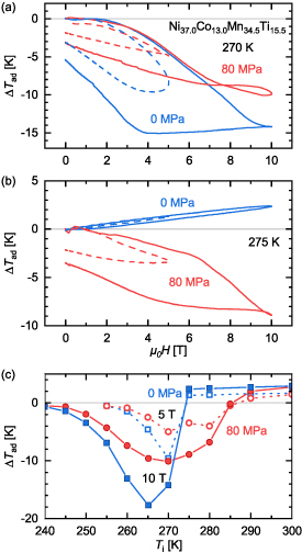
Figure 23. Adiabatic temperature change  in pulsed magnetic fields and under an uniaxial load of 0 and
  plotted in blue and red, respectively. Figures (a) and (b) show the field-dependent temperature change. (c) Maximum
  as a function of starting temperature. Data taken from [64].
Download figure:
Standard image High-resolution imageIf additional mechanical stress is applied, a whole series of changes occur in the system. The  peak for
  (see figure 23(c)) does not simply shift, but broadens asymmetrically towards higher temperatures with a reduced
  . As can be seen, for instance, in figure 23(b), there is an enormous influence of mechanical stress on the transition characteristics. For example, even though the Heusler alloy is already in the high-temperature phase at
  and
and  (indicated by the positive
  due to the conventional MCE of the austenite), a significant temperature drop is still observed under uniaxial load, with a change in slope around
  . This phenomenon could be pinned down to the special microstructure of the investigated Ni–Mn–Ti–Co alloy.
In the experiment, Heusler compounds were suction-cast into rods due to a higher fracture toughness compared to their simple arc-molten counterparts [46]. This mechanical strengthening is originating in the grain refinement during the suction-casting process, because of the accelerated solidification of the melt [87, 88]. However, this is highest at the edge of the cast cylinder and decreases towards its core. Optical and electron microscopy indicates that this results in preferential grain growth starting a few microns away from the outside to the inside in the shape of columnar grains. As the martensitic transition characteristics differ slightly between the core and shell of the rods, a two-step transition is observed in pulse-field experiments, which is intensified by applied pressure and a complex mechanical-stress field that evolves during the martensitic transformation. These findings demonstrate the intricacy of incorporating materials in multicaloric cooling cycles, as both intrinsic and extrinsic factors determine the attainable cooling performance significantly. Despite these complexities, the potential is immense, as we aim to illustrate in the following.
Typically, magnetocaloric demonstrator devices utilize permanent magnets and, thus, are limited to about  , which results in a maximum achievable temperature change of
  at best when using gadolinium [2, 89]. By implementing the active magnetic regenerator (AMR) principle, the temperature span can be increased. However, this is achieved at the cost of a decrease in cooling capacity [90–94]. In the end, the primary function of the magnetocaloric material is to pre-cool the final stage that removes heat from within the refrigerator. Considering the magnitude of
  in high fields, as illustrated in figure 11, this result is quite unsatisfactory. Pulsed magnetic fields can offer a solution, as they allow for the application of much higher fields, leading to higher
  , while maintaining manageable energy expenditure due to the short duration of the pulse. However, this also means that traditional heat-exchange designs cannot be used, as there is not enough time to transfer the heat from the magnetocaloric material to the exchange fluid.
With using a multicaloric material with hysteresis in the exploiting-hysteresis cycle, it is possible to access larger temperature changes. In this so-called hysteresis-positive approach (see figure 24) [85, 95], we first apply a magnetic field to a multicaloric material, such as a Heusler alloy exhibiting an inverse MCE, causing it to cool down. Then, due to an appropriately tuned thermal hysteresis, the reverse transition does not take place during demagnetization, as shown by step 2, which means that the material stays cold. After locking the material in its ferromagnetic phase in step 3, the heat can be absorbed by the material to cool down the system in the absence of a magnetic field. To return the material to its original state, a mechanical load is applied to shift the hysteresis curve to higher temperatures, and consequently the material transforms back into the low-temperature phase. This process is accompanied by a conventional elastocaloric effect, resulting in a substantial heating effect as the reverse transformation is induced (steps 4 and 5). The excess heat can then be expelled to the surrounding in step 6, the final step. The benefit of exploiting the hysteresis in this manner is that the temperature change is not reversed even after the magnetic field is removed, due to the nature of hysteresis.
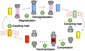
Figure 24. Schematic of the six-step exploiting-hysteresis cycle. The cylinders symbolize the multicaloric material and the blue, yellow, and red colors indicate low, ambient, and high temperature.
Download figure:
Standard image High-resolution imageHeusler alloys seem to be the ideal material class for this kind of application as they possess a tunable transition temperature and large hysteresis. Figure 25 shows the maximum  values for different Heusler alloys under moderate and high magnetic fields that have been studied at the HLD in the last couple of years [4, 96–99]. We provide comparison with gadolinium as well (conventional refrigeration approach). Among the Heusler alloys, the families Ni–Mn–In and Ni–Mn–In–Co are outstanding for their large
  in low fields and even reversible effects are obtainable in minor hysteresis loops [100]. The most essential reason for this is the huge shift of the transition temperature in magnetic fields
  , which can account for −10 K T−1 and more. In turn, this means that these materials are only of little use for high-field applications as their martensitic transition is already completed in small fields. Furthermore, a huge
  value results in a reduced entropy change of the complete transition
  due to the proportionality in the Clausius-Clapeyron equation [101]:

where  is the magnetization change during the FOT. As the entropy change is connected to the temperature via the specific heat, also
  is limited to about
  in Ni–Mn–In independent of the field (see figure 25).

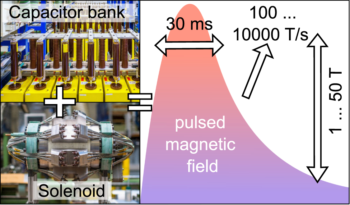
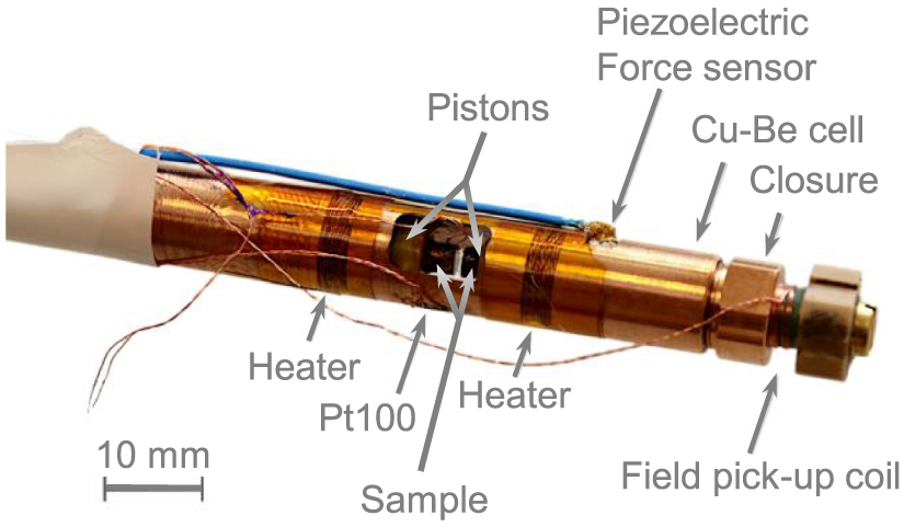
Figure 25. Measured  for a selection of Heusler alloys at 2, 5, 10 and 20 T. The corresponding transformation temperatures are always around room temperature. Results for gadolinium are plotted in the left of the plot. Data taken from [30, 44, 50, 60, 64, 102–104].
Download figure:
Standard image High-resolution image
In other Heusler alloys, such as Ni–Mn–Sn–Co and Ni–Mn–Ti–Co, the shift of the transition temperature with magnetic field is much smaller implying that higher field changes are necessary to complete the transition. For the later material family—the so-called all-d metal Heusler compounds—the adiabatic temperature change can achieve  for
for  [64]. During the reconversion, induced by uniaxial load, the material is warming by a similar magnitude allowing us to expel the heat to the surrounding. Such a temperature span would be sufficient for the operation of a single-stage multicaloric cooling device at room temperature instead of a 'multistage' AMR. The key is to properly tune the materials properties to the available magnetic-field change with sufficiently large hysteresis at the same time. However, the susceptibility of the transition to mechanical stress should be large as well in order to make the lowest possible pressures necessary to turn the material back into martensite so that the mechanical work to be applied remains low and fatigue can be avoided. The Ti-based Ni–Mn–Ti–Co Heusler alloys stand out in this respect as they show a robust compressive strength of
  or more and a sensitivity of the transition temperature to uniaxial load
  of about 200 K MPa−1. In summary, we can provide a list of requirements for materials operating in the exploiting-hysteresis cycle as follows:
- tunable transition temperature,
- modest shift of transition in magnetic field,
- large shift of transition in uniaxial load,
- large hysteresis,
- high mechanical stability,
- no fatigue.
It is, therefore, the task of future research to optimize materials in this direction. This is actually different from previous efforts in materials science, because the conventional approach has been to prepare compounds with the smallest possible hysteresis for use in low magnetic fields [49, 95]. The next stage in the development is to implement these novel materials into cooling devices in order to investigate their behavior in a real cooling cycle. Although there may be various challenges along the way, we are convinced that the effort is worthwhile to further advance the evolving field of solid-state refrigeration.
6. Conclusion
We presented an overview on the high-field characterization of magnetocaloric materials using pulsed magnetic fields at the Dresden High Magnetic Field Laboratory. We presented the technical details and discussed the most common experimental challenges encountered in pulse-field experiments and how to overcome them. Recent developments in the technique enable measuring the temperature change, strain, and magnetization simultaneously as well as the characterization of multicaloric materials under applied magnetic field and uniaxial load. We have shown that this is necessary to gain a comprehensive understanding of the materials properties. Through the discussion of different examples including the most relevant material classes in magnetocaloric research, we demonstrate how powerful the measurement method in pulsed magnetic fields is to study magneto- and multicaloric materials for future cooling applications.
Acknowledgments
It is our pleasure to thank M Acet, F Albertini, A Aliev, R Almeida, K Amirov, A Becker, B Beckmann, J Belo, L Beyer, L Caron, F Casoli, A Chirkova, L Cohen, P Devi, S Fabbrici, M Farle, C Felser, M Fries, K Friese, M Ghorbani-Zavareh, A Gràcia-Condal, M Gruner, O Gutfleisch, A Kamantsev, J Klotz, Yu Koshkid'ko, M Krautz, M Kuz'min, W Liu, Ll Mañosa, N Maraytta, Y Mudryk, A K Nayak, M Nicklas, L Pfeuffer, A Planes, F Scheibel, D L Schlagel, S Singh, K P Skokov, S Taskaev, A Taubel, A M Tishin, J Turcaud, N van Dijk, A Waske, B Weise, H Wende, S Yamamoto, and F Zhang who all contributed substantially to the work presented here. We especially thank the late Vitalij K Pecharsky.
This work was support by the Deutsche Forschungsgemeinschaft (DFG) through BEsT (Project-ID 456263705) and the Würzburg-Dresden Cluster of Excellence on Complexity and Topology in Quantum Matter– (EXC 2147, Project No. 390858490), the HLD at HZDR, member of the European Magnetic Field Laboratory (EMFL), the Helmholtz Association via the Helmholtz-RSF Joint Research Group (Project No. HRSF-0045), and the Clean Hydrogen Partnership and its members within the framework of the project HyLICAL (Grant No. 101101461).
Data availability statement
No new data were created or analyzed in this study.