
Abstract
Semiconductor spin qubits demonstrated single-qubit gates with fidelities up to  benchmarked in the single-qubit subspace. However, tomographic characterizations reveal non-negligible crosstalk errors in a larger space. Additionally, it was long thought that the two-qubit gate performance is limited by charge noise, which couples to the qubits via the exchange interaction. Here, we show that coherent error sources such as a limited bandwidth of the control signals, diabaticity errors, microwave crosstalk, and non-linear transfer functions can equally limit the fidelity. We report a simple theoretical framework for pulse optimization that relates erroneous dynamics to spectral concentration problems and allows for the reuse of existing signal shaping methods on a larger set of gate operations. We apply this framework to common gate operations for spin qubits and show that simple pulse shaping techniques can significantly improve the performance of these gate operations in the presence of such coherent error sources. The methods presented in the paper were used to demonstrate two-qubit gate fidelities with
  in Xue et al (2022 Nature601 343). We also find that single and two-qubit gates can be optimized using the same pulse shape. We use analytic derivations and numerical simulations to arrive at predicted gate fidelities greater than 99.9% with duration less than,
  where
where  is the difference in qubit frequencies.
Export citation and abstract BibTeX RIS

Original content from this work may be used under the terms of the Creative Commons Attribution 4.0 license. Any further distribution of this work must maintain attribution to the author(s) and the title of the work, journal citation and DOI.
1. Introduction
Spin qubits based on electrons confined in quantum dots (QDs) [1] are a leading candidate for long-term applications in quantum information processing. They provide long relaxation times [2–12] and their lithographic fabrications allow for dense and scalable qubit architectures [13, 14]. Using isotopically enriched silicon (Si) [15] or germanium (Ge) [16] in favor of gallium arsenide (GaAs) [1] as the host material for the QDs allows for significant longer decoherence times due to the low abundance of nuclear spins. One common feature of all spin qubits is the need for electric control on the nanoscale, which typically also couples the system to electrical noise.
Depending on the host material, single-qubit gates are either implemented using electron spin resonance (ESR) [17–19] or electric-dipole spin resonance (EDSR) [20–26] by applying microwave signals at the qubit resonance frequency.
All-electrical two-qubit gates can be implemented using dc gate voltage pulses that switch on and off the exchange interaction [27]. However, the originally proposed universal  gate [27] was found to be impractical to yield high fidelities. The reason is that qubit frequency differences of typically tens of MHz are engineered to facilitate qubit addressability [13]. A high-quality
  gate requires J much larger than the qubit frequency differences [28, 29], so
  MHz. This regime typically can only be accessed away from the symmetric operation point, where charge noise introduces strong dephasing [10, 30, 31]. In the presence of such non-vanishing qubit frequency differences,
  not much less than J, the adiabatic cz gate offers a practical alternative. The adiabatic cz gate, where a conditional phase difference is acquired by an adiabatic exchange pulse, is less demanding to hardware at the cost of longer gate times [29]. Two-qubit gates with fidelities
  [32–35] were recently reported, with the highest fidelities reported using the adiabatic cz gate [32, 35].
Even without the presence of decoherence, qubit operations can be subject to errors. These coherent errors can arise from miscalibration, crosstalk, non-adiabaticity, finite bandwidths, filtered signals, non-linear transfer functions, from certain approximations made such as the rotating wave approximation, and many other spectator and control errors [13]. Depending on the specifics, coherent errors can easily be larger than those from decoherence.
The standard approach for mitigating these errors is summarized in optimal control theory [36] which can be divided into three main approaches. Firstly, a geometric approach that rewrites the time evolution into Pontryagin's Maximum Principle [37]. The optimal control pulse is then given by the extreme conditions that satisfy the given boundary conditions. However, analytical solutions are mostly limited to small and simple systems. A recent extension to this approach is the space curve quantum control (SCQC) formalism [38] that can also deal with incoherent errors. Secondly, fully numerical techniques, such as the GRAPE [39] and CRAB algorithms [40], can be used to find a (hopefully) global minima of the error by varying parameters of the input signal. This comes at the cost of speed and flexibility to small modifications. Lastly, inherent error mitigation can be achieved via (enforced) adiabatic dynamics [41–45].
In this paper, we want to provide a simple framework to reduce coherent errors based on the adiabatic approach. We start in section 2 by introducing a framework which allows us to separate the desired dynamics, which is the target gate, from erroneous dynamics that yields gate errors. We also show how existing methods from the literature [42–44] are captured within this framework and can be reapplied to a larger set of gate operations. We then apply this framework in section 3 to derive optimized pulse shapes that reduce the errors on the most widely used single- and two-qubit gates for spin qubits. Subsequently, in section 4, we numerically demonstrate the effectiveness of the derived pulse shapes in the presence of incoherent noise sources and benchmark them via the average gate fidelity. Throughout the paper, fidelity always refers to the average gate fidelity. By significantly reducing the magnitude of coherent errors, our simulations show that gate fidelities  with duration less than 50 ns are feasible.
2. Framework for optimizing pulse shapes
Figure 1 displays our general framework for finding optimized pulse shapes to mitigate coherent errors. We start considering a quantum system with a Hilbert space  which is described by a Hamiltonian H(t) of dimension n × n. Ignoring any incoherent dynamics, the time-evolution from t = 0 to a final time t generated by the Hamiltonian is described by a propagator U(t) that solves [49]


where  is the derivative of U with respect to time t. Its formal solution at
  is the time-evolution operator given by

where  denotes the usual time-ordering. We imply that U describes an operation which is close to an ideal or a targeted operation described by the unitary operation Uideal. We can now define the error propagator as

The standard approach of estimating the errors is by measuring the average gate fidelity of the erroneous operation [50]

where d is the dimension of the Hilbert space. For a noisy process described by a superoperator χ we replace  in equation (5). There are two standard approaches to experimentally access the gate fidelity, process tomography [51] and randomized benchmarking [52], both requiring complex circuits and analysis and either susceptible to state preparation and measurement (SPAM) errors or limited in the information gain. However, much progress has been made to increase the information gain and reduce the susceptibility to SPAM errors, e.g. using gate set tomography (GST) [53] and shadow tomography techniques [54].

Figure 1. (a) Flowchart of the proposed framework for gate optimization. The system Hamiltonian H is separated into an ideal part covering the dominant interaction and a small erroneous part consisting of imperfections. After transforming into the interaction frame with respect to Hideal a Magnus expansion is performed to compute the error rates. (b)–(d) Mitigation strategies to reduce coherent errors, shown for the example of a single-qubit  gate in a double-dot system with qubit frequency difference
  MHz. (b) Simulated infidelity of the gate operation as a function of the pulse-length, with a control Hamiltonian that is instantly turned on and off with (blue) and without (orange) filtering. Minima correspond to the synchronization condition (see [46, 47]). (c) Simulated infidelity of the gate operation as a function of the pulse-length for different filtered pulse shapes optimized to concentrate the energy spectral density [48]. (d) Simulated infidelity of the gate operation as a function of the pulse-length using a filtered Hann window with (blue) and without (orange) additional dynamic pulse shaping [42]. Simulation parameters are discussed in appendix
Download figure:
Standard image High-resolution image2.1. Separating erroneous and ideal dynamics
Assuming the time dynamics of the targeted gate is known for each time ![$t\in[0,t_g]$](https://content.cld.iop.org/journals/2058-9565/8/4/045025/revision2/qstacf786ieqn18.gif) , we can now equally define the erroneous dynamics based on equation (4) as
, we can now equally define the erroneous dynamics based on equation (4) as

We can find the corresponding ideal and error Hamiltonian by plugging  into equation (1) to arrive at [49, 55]

Additionally, Uideal and Hideal are related via the time-ordered exponential

Consequently, the associated ideal and error Hamiltonian are then given by [56]


The formal solution to equation (7) at  is again the time-ordered exponential given by


From the first to the second line we applied the Magnus expansion with Magnus coefficients  . We further assume small errors
 ![$\underset{t\in [0,t_g]}{\text{max}}||H_\text{error}(t)||_2\ll \hbar \pi/t_g$](https://content.cld.iop.org/journals/2058-9565/8/4/045025/revision2/qstacf786ieqn22.gif) , where
, where  denotes the spectral matrix norm, (otherwise we choose a closer desired gate) to ensure a fast converging Magnus series. In the last step, we truncated the Magnus expansion at lowest order. We show later that this order is sufficient to find parameters for quantum operations with gate fidelities in the order of
  for three important applications. Since we assumed small errors, we can also expand the matrix exponential equation (13) up to linear order

As a matter of fact, our error matrix corresponds to the Hamiltonian errors of the error generator [57] defined as  , where χ is a superoperator that can be measured with quantum process tomography techniques. Furthermore, an analogous derivation can be performed if incoherent errors are included by replacing the system Hamiltonian with a stochastic Hamiltonian [58] or Liouvillian. We leave this to a future investigation and focus in this work on coherent errors.
2.2. Erroneous dynamics
To achieve a high-fidelity quantum gate we rewrite equation (14) into a minimization condition

There are multiple approaches to finding the minimum, such as brute force numerical Nelder-Mead [59], GRAPE [39] and CRAB algorithms [40] or a parameterization of the integration path [38, 45]. In general, there are n2 free real parameters of a Hermitian matrix (or unitary matrix) that need to be optimized.
In this work, we use a different approach that makes use of two properties that are common in many quantum computing device architectures, sparse interactions and a priori knowledge of the system, that allow us to greatly increase the efficiency of finding optimized pulse shapes. Instead, we use the equivalence of matrix norms to rewrite equation (15) as

where the error channels Ok
with  describe a full basis set of n × n operators. A smart choice of the channels
  can often allow us to truncate the series after a few terms with minimal consequences. The error channels Ok
can be constructed from the a priori knowledge of the system, either through fast tomographic methods [60] or through a trustworthy theoretical model. We focus in this paper on the latter.
can often allow us to truncate the series after a few terms with minimal consequences. The error channels Ok
can be constructed from the a priori knowledge of the system, either through fast tomographic methods [60] or through a trustworthy theoretical model. We focus in this paper on the latter.
We find the choice  with
with  to work well, where
  are eigenstates of a dynamic invariant I(t) with respect to the ideal dynamics Uideal. The dynamic invariant is a Hermitian operator I(t) that satisfies
 ![$i\hbar \dot{I}(t) = [H_\text{ideal}(t),I(t)]$](https://content.cld.iop.org/journals/2058-9565/8/4/045025/revision2/qstacf786ieqn31.gif) with
with ![$[H_\text{ideal}(0),I(0)] = 0 = [H_\text{ideal}(t_g),I(t_g)]$](https://content.cld.iop.org/journals/2058-9565/8/4/045025/revision2/qstacf786ieqn32.gif) , where
, where ![$[A,B] = AB-BA$](https://content.cld.iop.org/journals/2058-9565/8/4/045025/revision2/qstacf786ieqn33.gif) [61]. We note that
[61]. We note that ![$[H_\text{ideal}(t_g),I(t_g)] = 0$](https://content.cld.iop.org/journals/2058-9565/8/4/045025/revision2/qstacf786ieqn34.gif) is not required in general, but guarantees state transfers without final excitation. This allows us to conveniently decompose the ideal dynamics as [62]
is not required in general, but guarantees state transfers without final excitation. This allows us to conveniently decompose the ideal dynamics as [62]

where the phase αm is the Lewis–Riesenfeld phase

While finding the dynamic invariant I(t) in the general case is hard, there are two special cases of interest that allow for a great simplification. If Uideal describes an adiabatic dynamic or if ![$[H_\text{ideal}(t_1),H_\text{ideal}(t_2)] = 0$](https://content.cld.iop.org/journals/2058-9565/8/4/045025/revision2/qstacf786ieqn35.gif) for all
for all ![$t_1,t_2\in [0,t_g]$](https://content.cld.iop.org/journals/2058-9565/8/4/045025/revision2/qstacf786ieqn36.gif) , one can find a common set of eigenstates for
, one can find a common set of eigenstates for  and I(t). In the latter case, the eigenstates are time-independent,
  , and also eigenstates of
  . Therefore, the phase can be simplified to
  , where
  is the mth eigenenergy of Hideal. Note that all practical applications discussed in section 3 fall in the latter case. For the adiabatic case, one has also to add the geometric phase [56].
Using the dynamic invariant decomposition, we can now rewrite the error Hamiltonian into a complex parameter  , the phase
  [62], and time-independent matrix elements

Here the complex parameter

describes the transition matrix element caused by the erroneous dynamics. Similarly, we find  to be the difference of the associated Lewis–Riesenfeld phases

In summary, the decomposition of the error Hamiltonian into operators  allows us to 'measure' the deviations from the ideal dynamics and quantifies the probability of making a coherent error generated by
  [57]. The associated error rate is then given by

with  and
and  . In the language of pulse optimization,
  is the control signal. For later convenience, we also define a corresponding frequency

The error rates can be related to the problem of transmitting a signal through a channel with finite frequency bandwidth. This can be shown by substituting [48, 63]

with a constant  and assuming
  . By choosing
  , the static parameter
  can be seen as the averaged resonance frequency over the time interval
  ] of the ideal system,
  . In certain scenarios it might be beneficial to fix
  equal to characteristic frequencies such as the idle resonance frequencies instead and allow
  . In this manuscript, we use the upper convention. In both cases, the relation between real time t and dilated normal time s is given by integrating equation (24) arriving at [48]


The inverted functions are best acquired using numerical interpolation [48], e.g. Mathematica directly provides  using the command
 ![$\text{Interpolation}[\text{Table}[\lbrace t[s], \tilde{g}[s]\rbrace, \lbrace s, 0, 1\rbrace]]$](https://content.cld.iop.org/journals/2058-9565/8/4/045025/revision2/qstacf786ieqn60.gif) with sufficient sampling.
with sufficient sampling.
For the following discussions, we focus on a single error rate, thus dropping the index k to increase readability. We can rewrite the error rate in equation (22) using the substitution (24) as


with  and the associated energy spectral density S. From the first to second line, we replaced the integral which corresponds to a short-time Fourier transformation with the expression for an energy spectral power of the input signal
  [48]. As a consequence, we have now shifted the task from minimizing the error rates to optimizing the energy spectral density, a task investigated in the field of signal processing, and which has been solved for many input signals. Below, we show a few examples of how signal processing can be used for finding optimized pulse shapes.
2.3. Optimization strategies
2.3.1. Synchronization
Since in quantum mechanics, most coherent processes are periodic, the simplest approach to minimize the error is to investigate the frequency of these processes. Due to the finite gate time tg
, equation (28) is always an oscillatory function with respect to  if
if  . This can be shown using the convolution theorem. We rewrite the input signal
  , where
  is the unit box function. This allows us to replace the short-time Fourier transformation with the conventional Fourier transformation. The resulting Fourier transform is clearly oscillating due to
 ![$\mathcal{F}[\Pi(0,t)] = \sin(x)/x$](https://content.cld.iop.org/journals/2058-9565/8/4/045025/revision2/qstacf786ieqn67.gif) , where
, where  denotes the Fourier transform. We now make use of the oscillating pattern using synchronization.
Synchronization is the concept of finding minima of equation (28) which due to the oscillatory pattern exist, see for example figure 1(b). The optimal pulse length tg
or system parameter νf
are then given by the minima of  . The concept of synchronization is best visualized in the special case of constant f(t) and g(t). Such a constant pulse with infinite fast turn-on, conventionally called rectangular window, allows achieving
  in the shortest time.
These minima correspond to cases where the undesired interaction 'undoes' itself for specific combinations of νf and tg . For example, the swap oscillation frequency can be synchronized with the conditional phase evolution such that a CZ can be implemented [28] or off-resonant Rabi oscillations can be synchronized with resonantly driven single-qubit gates [46, 47]. An advantage of this strategy is the absence of any complex pulse shaping. However, the requirement for simultaneous minima in the spectrum makes it difficult to scale beyond a handful of qubits [47, 64]. Additionally, filtering in the signal transmission greatly reduces the effectiveness of the performance of gate operations (see figure 1(b) using a simple low-pass filter).
2.3.2. Static pulse shaping
We first discuss pulse shaping techniques in the case of a single experimental control parameter, e.g. baseband signals, corresponding to real transition matrix elements g(t) (constant phase factors can be factored out). In this case, fast operations with consistently low error rates can be achieved using window functions w(t) designed for optimized spectral concentration such as the discrete prolate spheroidal sequence (DPSS or Slepian), and the Dolph–Chebyshev window. Alternatively, if faster operations at the cost of larger coherent errors are desired, a Hamming window is the best choice. Unfortunately, the optimized window functions typically require a high computational cost, high bandwidth, and high time-resolution, thus restricting their practical use. Therefore, in practical applications in quantum computing, often approximations of the optimized windows are used, which reach almost equally small errors. An example is the Kaiser window that is often used to replace the DPSS window [65]

Here,  is a normalization constant defined via
  and
and  is the 0th order modified Bessel function. Alternatively, one can also use a Fourier series [48]

with the even and odd decomposition


The optimal Fourier coefficients ![$\left.\lambda_{\text{even}} = [1.0715,-0.0795,0.0043,0.0037]\right.$](https://content.cld.iop.org/journals/2058-9565/8/4/045025/revision2/qstacf786ieqn74.gif) and
and ![$\left.\lambda_{\text{odd}} = [0,0,0,0]\right.$](https://content.cld.iop.org/journals/2058-9565/8/4/045025/revision2/qstacf786ieqn75.gif) can be estimated from a Fourier expansion of the Slepian window or from direct numerical minimization of the error rate [48]. This approach has the advantage that by using only even components, a smooth pulse shape and
can be estimated from a Fourier expansion of the Slepian window or from direct numerical minimization of the error rate [48]. This approach has the advantage that by using only even components, a smooth pulse shape and  is guaranteed.
A simple and popular pulse shape is the Hann window (sometime also cosine window) (![$\left.\lambda_{\text{even}} = [1,0,0,0]\right.$](https://content.cld.iop.org/journals/2058-9565/8/4/045025/revision2/qstacf786ieqn77.gif) ) or its generalization the Tukey window defined as [32]
) or its generalization the Tukey window defined as [32]

The Tukey window consists of two halves of a Hann window interleaved by a constant part and is formally the convolution of the Hann window and a rectangular window. For λ = 1 it reduces to the Hann window. Both the Hann and the Tukey window have the advantage that they can easily be synchronized due to their pronounced oscillatory spectral density. An interesting thought is also combining the Tukey window shape with the Fourier approximation, which we will leave for future investigations.
Once decided on a preferred pulse shape, the optimal pulse design to minimize the error rate is then given by setting

The amplitude A has to be estimated from the desired gate operation (9).
Figure 1(c) shows the resulting infidelity of a gate operation for different pulse shapes. As designed, the Kaiser window outperforms the Tukey and Hann windows in terms of performance, but the latter may be simpler to implement.
2.3.3. Dynamic pulse shaping
Next, we discuss the case of two orthogonal experimental control parameters, e.g. microwave amplitude and phase, corresponding to complex matrix transition elements,  . In this case, the steps for the upper mitigation strategies have to be simultaneously applied for the real and imaginary part. Again, the trivial case
  corresponds to a single control parameter and the constant phase factor can be factored out. In the general case, the upper methods may fail since the solutions for the real and imaginary components may be incompatible.
Such non-trivial complex matrix transition elements appear for example in the case of resonantly driven gates, i.e. single-qubit gates for spin qubits [12], controlled rotation gates [46], or simultaneous pulsing of both barrier gates for exchange-only qubits [12]. Within the rotating wave approximation, the phase of the MW signal translates into complex matrix transition elements  . Here,
  is the real and
  the imaginary part corresponding to the I/Q quadrature of the MW signal.
Fortunately, such complex signals can actively be used to significantly reduce the error rates compared to window functions [44] by making full use of the additional degree of freedom. For example, the derivative removal by adiabatic gate (DRAG) [42, 66] and Wah-Wah [67–69] protocols both allow to suppress crosstalk from off-resonant drives beyond what conventional window functions can achieve. These protocols can be visualized by integrating equation (27) by parts with respect to the real part of the signal [70]

with boundary conditions  . We get a complete cancellation of the error rate with

where the pulse shape of  can individually be optimized using window functions.
Figure 1(d) shows that using dynamic pulse shaping protocols (here DRAG) significantly reduces the error rate. For  this exactly yields the DRAG condition
  . The advantage of this strategy is a strong suppression of the error rate at the cost of additional power consumption, which scales with the number of suppressed transitions [71]. Our framework allows generalizing this powerful method beyond microwave control to all systems with independent control over two orthogonal axes.
3. Applications
In this section, we show explicit applications of our framework by optimizing important spin qubit operations.
Before we turn to the actual optimization, we introduce the theoretical description of a spin qubit system. We restrict ourselves here to spin- qubits encoded in electrons or holes with weak spin-orbit interaction. The dynamics of electron spins in the
  charge configuration of a multi-qubit network can be well-described by the Heisenberg model [27] (see also appendix

Here,  is the vector consisting of spin matrices, where
  is the Pauli matrix acting on the spin in dot j and
  is the magnetic field felt by the electron in dot j. For later convenience, we define the average field
  and the difference field
  . Note that in this notation, the magnetic field
B
and the exchange interaction J are in units of GHz.
. Note that in this notation, the magnetic field
B
and the exchange interaction J are in units of GHz.
Single-qubit gates are typically operated in the regime of negligible exchange interaction, J ≈ 0, a finite static magnetic field  that sets the qubit resonance frequency, and are implemented via resonant driving using ESR or EDSR. Here, we do not distinguish between the two mechanisms and describe both by an (effective) oscillating magnetic field
  , such that
  . We discuss here the case of two qubits driven by a single microwave tone, but note that our framework can also treat simultaneous operations as well as multi-qubit systems.
Exchange-based two-qubit gates are operated in the regime of J > 0. For simplicity, we assume that all two-qubit gates are operated deep inside the (1,1) charge occupation regime at the symmetric operation point and electric control is maintained via virtual barrier gates [10, 32, 72].
Theoretically, we describe the combined system using Hamiltonian (37) and move into a rotating frame ![$R = \exp[- i (2\pi\nu_D t+\theta) (S_{1}^z+S_{2}^z)]$](https://content.cld.iop.org/journals/2058-9565/8/4/045025/revision2/qstacf786ieqn97.gif) of both spins. In the standard basis
of both spins. In the standard basis  (
( and
and  correspond to ground and excited qubit state) to the following Hamiltonian

where νD
is the drive frequency, θ the phase of the drive, and  the perpendicular component of the magnetic field felt by qubit
  with respect to the quantization axis.
3.1. Resonant single-qubit gates
We first optimize single-qubit operations. Expected coherent errors for resonantly driven single-qubit gates are crosstalk and related spectator errors. For example, off-resonant driving due to microwave leakage or shared driving gates [73], non-linear driving and their impact such as higher harmonic generation [74], phase shifts and frequency shifts [75], and the impact of counter-rotating driving such as Bloch Siegert shifts [76]. To include non-linear driving effects into our theoretical description, we expand the modulated (effective) magnetic field  in terms of a Fourier series with respect to the drive frequency νD
, where the Fourier components
in terms of a Fourier series with respect to the drive frequency νD
, where the Fourier components  and
and  are assumed to be slowly varying in the time interval
  .
.
The Hamiltonian can be significantly simplified under the rotating wave approximation (RWA) where we keep stationary terms and disregard all terms which are modulated with frequency  with
with  . Corrections from violations of the RWA scale with
  and are negligible for typical experimental conditions. However, higher-order corrections can become important for ultra-fast gate operations [77, 78] or driving at comparatively low frequencies [17].
In this section, we focus on the RWA case and leave the general investigation to the future. Corrections beyond the RWA can be included by using directly Hamiltonian (38) instead, or by applying the generalized RWA introduced in [79] and discussed in section 3.3 and appendix
We use the following Hamiltonian as a basis for our pulse optimization framework

where we kept time-dependent phases to account for shifts in resonance frequency.
Next we describe our targeted ideal operation [21] as

with frequency detuning  and find Herror via equation (10). Our target gate operation describes a single-qubit Rabi oscillation on qubit Q1 and phase shifts on the non-driven qubit Q2. We include the largest expected error, a phase accumulation (Sz
2) on the non-driven qubit known as ac Stark shift, into our target operation to keep the erroneous evolution small. Such phase-shift can be corrected easily via a virtual z gate on Q2 in an experimental realization.
and find Herror via equation (10). Our target gate operation describes a single-qubit Rabi oscillation on qubit Q1 and phase shifts on the non-driven qubit Q2. We include the largest expected error, a phase accumulation (Sz
2) on the non-driven qubit known as ac Stark shift, into our target operation to keep the erroneous evolution small. Such phase-shift can be corrected easily via a virtual z gate on Q2 in an experimental realization.
We find (see appendix C.1) two pairs of dominant error channels described by the operators  and
and  with erroneous evolutions


desired evolutions


and error rates


The first error rate describes a shift in the rotation axis (x-direction) of qubit 1 giving rise to Sy
1 and Sz
1 errors. The best mitigation strategy is dynamic pulse shaping via a time-dependent phase  , e.g. through chirping [80, 81]. The second error rate describes a spin-flip of the second qubit due to off-resonant driving, giving rise to Sx
2 and Sy
2 errors. The mitigation of the spin-flip errors requires either synchronization or dynamic pulse shaping.
, e.g. through chirping [80, 81]. The second error rate describes a spin-flip of the second qubit due to off-resonant driving, giving rise to Sx
2 and Sy
2 errors. The mitigation of the spin-flip errors requires either synchronization or dynamic pulse shaping.
The condition for the synchronization of a  gate on qubit j affecting qubit i (i ≠ j) with a rectangular pulse shape is (see also [47])

with integer m and n. The condition for a synchronized  gate is given by the substitution
  . For minimal gate time assuming an equally strong global drive
  , the synchronization condition for a
  gate is simplified to

which corresponds exactly to the minima in figure 1(b).
For static pulse shaping,  and
and  , constant drive frequency
  , and negligible shift in resonance frequency
  , the first error rate equation (45) vanishes, and we only need to minimize equation (46) which is simplified to

Optimal pulse shapes for a  gate are then given by
  , where we use the normalized window
  . Figure 1(c) displays the simulated infidelity for different pulse shapes as a function of gate time tg
.
. Figure 1(c) displays the simulated infidelity for different pulse shapes as a function of gate time tg
.
Under the same assumptions such as constant drive frequency  and negligible shift in resonance frequency
  , dynamic pulse shaping provides even faster gate times with small errors (see figures 1(c) and (d)). Applying the DRAG method [42] equations (45) and (46) combined with a Hann window, the optimized dynamic pulse shape is (see figure 1(d))


The renormalization of the drive amplitude is due to the additional power in driving. The optimized pulse shape for driving qubit 2 is given by substituting  in equations (50)–(52).
3.2. Exchange-based two-qubit cz gate
Next, we optimize the two-qubit gate. A crucial condition for high-fidelity two-qubit cz gates is an adiabatic turn on/off or pulse of the exchange interaction, which can give rise to substantial errors if violated [32]. While in principle an echo pulse sequence allows suppressing non-adiabatic errors [46] for a cz gate, the echo pulse is often inconvenient and introduces additional noise through the longer gate sequences.
Starting from Hamiltonian (38) we notice that the exchange interaction only affects the odd parity states  (see appendix
  ,
,  , and
, and  , we find

We define the targeted ideal gate as

which implements up to single-qubit phases a cz-gate at the time  . Here, the unitary
  diagonalizes Hamiltonian (53) with resonance frequency
  and
and  . Our target operation describes the adiabatic phase evolution due to the exchange interaction.
There is (see appendix C.2) a single dominant error channel causing swap-oscillations [28] that is described by the spin-flip operator  , where
  and
and  are the eigenstates of Hamiltonian (53). The erroneous and targeted time evolutions are


For small exchange  and constant Zeeman splitting
  we can simplify
  and
and  to find the error rate

Remarkably, this optimization condition for an adiabatic cz gate is identical to the condition for minimizing single-qubit crosstalk in equation (49) under the replacement  with the same invariant
  . The conditions for the synchronization of a cz gate with a rectangular pulse shape and minimal time tg
is [28]
. The conditions for the synchronization of a cz gate with a rectangular pulse shape and minimal time tg
is [28]

with integer m. Here  is the difference in resonance frequency during the pulse. Note that this is equivalent to the synchronization condition of a
  gate (see equation (48)).
We show later that static pulse shaping is sufficient to get error rates for the cz-gate below  . Due to the non-linear relation between barrier voltage and exchange interaction (see appendix
  is then given by (see appendix


using the relation between real-time t and time s. The amplitude A is given by the conditional phase condition  . For
. For  and constant Zeeman splitting
  we find

where we use  and the normalized window
  .
.
3.3. Exchange-based two-qubit resonant swap gate
Another set of two-qubit gates can be accessed by driving the exchange interaction directly at the  resonance frequency
  [82, 83]. This gate exchanges the population (swapping) between the two states. For the resonant swap gate, dominant coherent errors are violations of the rotating wave approximation due to
  MHz and the influence of higher harmonics due to the non-linear voltage-exchange relation.
In general, driving the barrier voltage yields  , which gives rise to


where we have expressed J and  in terms of Fourier coefficients with respect to the drive frequency
  . Due to the impact of the barrier voltage on the resonance frequency [32], we consider in our model
  with
with  .
.
Without loss of generality, the dynamics is again projected on the odd-parity subspace spanned by  and described by Hamiltonian (53). To simplify the Hamiltonian, we perform a double basis transformation
  before we apply our framework. The first transformation diagonalizes Hamiltonian (53) at t = 0, and the second moves us into the rotating frame with respect to the driving frequency and driving phase. The transformed and rotated Hamiltonian reads

Within this frame, the target operation is then given by [82]

which describes swap oscillations between the basis states.
We find (see appendix C.3) a single pair of error rates described by the operators  . The erroneous transition matrix elements and the accumulated energy gap are then


3.3.1. General case
In the general case, no closed-form analytical expressions can be derived for equation (62) and one has to rely on numerical techniques. Unfortunately, we cannot use the substitution (24) for the general Hamiltonian since f = 0 and proceed directly to the mitigation methods and omit the substitution. However, we note that all steps in our framework can be applied if we apply a (generalized) RWA [79] on Hamiltonian (64) to remove the oscillating components.
Our framework tells us for non-trivial complex matrix transition elements  to use dynamical pulse shaping. We separate them into real gR
and imaginary gI
components and then perform integration by parts
to use dynamical pulse shaping. We separate them into real gR
and imaginary gI
components and then perform integration by parts


where  is given by the antiderivative of f(t) (see equation (24)). Here, we restrict ourselves to solutions where the limits of integration vanish at
  . The optimized
  is the solution of the integro-differential equation for the phase θj
by plugging in equations (66) and (67).
is the solution of the integro-differential equation for the phase θj
by plugging in equations (66) and (67).
3.3.2. Exponential exchange
We now consider the case of an exponential interaction  and linear frequency shifts,
  . This regime is experimentally accessed in [82, 83]. In this limit, exact analytical expressions can be derived. The Fourier coefficients are given by

for  , where
  denotes the modified Bessel function of order k. In this special case, the optimized dynamic pulse shape can be explicitly expressed

with the dynamic phase

The first term originates from the conventional RWA and compensates the shift in resonance frequency  due to non-linear exchange. The remaining term describes the driving-induced shift of the rotation angle and can be derived using a generalized RWA [79] (see appendix
4. Performance
In this section, we show that the aforementioned techniques lead to high-fidelity single- and two-qubit gates. We benchmark the gates by computing the time-evolution of an input state  by step-wise integration of the Schrödinger equation,

where H(t) is the exact Hamiltonian (38) in the rotating frame without neglecting the counter-rotating terms. Noise is added in two ways into the dynamics. Because of its slow dynamics compared to the gate times  s, magnetic noise affecting the single spins is simulated by a quasi-static shift of the qubit resonance frequencies
  . Explicitly, we used
  with
with  and
and  kHz from [32]. Charge noise on the electrodes,
  , typically introduces smaller errors, but must be included when operating at the symmetric operating point, where voltage fluctuations affect the exchange interaction. Charge noise is simulated using colored noise with a spectral density
  using the Fourier Filter method [84, 85].
4.1. Resonant single-qubit gates
Each large-scale qubit device needs consistently small single-qubit error rates to fulfill the requirements for error correction [86, 87]. A frequently reported number are infidelities of  for the physical gate operations [86, 88], although based on many assumptions such as good initialization and readout and uncorrelated errors. Our simulations show that sufficiently small infidelities are within reach on state-of-the-art qubit devices using our framework. The simplest technique, synchronization of the Rabi-frequencies [46, 47], already shows small infidelities in our simulations. However, low-pass filters built into the electronic circuits to reduce high-frequency noise, are a detrimental error source for the synchronization technique. This is seen in figure 1(b) that shows the infidelity with (blue) and without (orange) a 150 MHz-Butterworth filter. The filter significantly reduces the dips as well as shifts the minima. On the other hand, our simulations (see figures 1(c) and (d)) show that high-fidelity operations can still be reached using static or dynamic pulse shaping to reach infidelities as small as 10−4 for gate times in the order of
  ns with a frequency separation of
  MHz. Note, that this, on the one hand, directly implies that gate times
  ns are required if the frequency separation is reduced to
  as proposed in some architectures, e.g. [13]. On the other hand, a larger frequency separation allows for faster high-fidelity gate operations [35, 89] due to the infidelity being invariant for
  . In the former case, dynamic pulse shaping, such as the derivative removal by adiabatic gate (DRAG) protocol [42, 66], allows for an additional improvement.
4.2. Exchange-based two-qubit cz gate
Many experiments on single-spin qubits use the universal cz gate [28, 29] as their native high-fidelity two-qubit gate [19, 24, 32, 33, 35, 90] due to its simplicity and potential for scaling to larger arrays [26, 73]. The cz-class (cphase) gate


with  can be directly acquired using only single-qubit phase gates
1
from the adiabatic phase evolution under the exchange interaction and can be transformed into a cnot gate using two single-qubit
can be directly acquired using only single-qubit phase gates
1
from the adiabatic phase evolution under the exchange interaction and can be transformed into a cnot gate using two single-qubit  gates. For the cz gate, the exchange interaction J(t) is pulsed, picking up a conditional phase
  with integer n. Since the cz gate is intended to be adiabatic innately, it is also directly (linearly) susceptible to low-frequency noise acting on the resonance frequencies. However, we claim that a substantial error in previous realizations [19, 91] is due to violations of the adiabaticity condition, which is more severely impacted due to the non-linear voltage-exchange relation and gives rise to bit-flip errors. Here, the adiabaticity condition is with respect to the frequency difference
  between the two spin qubits. Since the coherent errors of a cz two-qubit and resonant single-qubit gates are related and
  is an invariant in the simulations, we know that the cz gate can, for example, be further improved using the Kaiser window or increasing the separation in qubit frequency. Figure 2(a) shows the simulated infidelity of a cz gate as a function of gate time tg
and the proportionality factor
is an invariant in the simulations, we know that the cz gate can, for example, be further improved using the Kaiser window or increasing the separation in qubit frequency. Figure 2(a) shows the simulated infidelity of a cz gate as a function of gate time tg
and the proportionality factor ![$\alpha\in [0,1]$](https://content.cld.iop.org/journals/2058-9565/8/4/045025/revision2/qstacf786ieqn194.gif) from the Tukey window, see equation (33). The oscillating infidelity as a function of exchange corresponds to an interference pattern of the diabatic contributions identical to the one observed in figures 1(b) and (c). On the other hand, a small frequency separation severely limits the performance, since long gate times
from the Tukey window, see equation (33). The oscillating infidelity as a function of exchange corresponds to an interference pattern of the diabatic contributions identical to the one observed in figures 1(b) and (c). On the other hand, a small frequency separation severely limits the performance, since long gate times  are required if the frequency separation is reduced to
  [92, 93]. In situations with a small frequency separation, a non-adiabatic cz gate can be realized as shown theoretically [28] and demonstrated experimentally [91] using the synchronization condition. Our simulations confirm such high-fidelity gates in figure 2(a) for λ = 0, where the Tukey pulse corresponds to a rectangular pulse. However, the diabatic implementation requires a precise timing, is sensitive to pulse imperfections such as filter effects, and is prone to dephasing due to low-frequency noise.

Figure 2. (a) Simulated noiseless average gate infidelity  for a cz gate as a function of pulse length tg
and the shaping factor λ of the Tukey window equation (33) (same colorbar as in (b)). The star highlights the pulse shape used in [32] demonstrating
for a cz gate as a function of pulse length tg
and the shaping factor λ of the Tukey window equation (33) (same colorbar as in (b)). The star highlights the pulse shape used in [32] demonstrating  in isotopically enriched silicon quantum dots. (b) Simulated infidelity
  for a cz gate as a function of pulse length tg
and charge noise acting on the virtual voltage considering
for a cz gate as a function of pulse length tg
and charge noise acting on the virtual voltage considering  with amplitude A using a Hann window (λ = 1). The dashed lines highlight the value of extracted charge noise and pulse duration from [32]. Single-qubit noise is added as quasi-static fluctuations with amplitudes taken from [32].
Download figure:
Standard image High-resolution imageWe now compare our results to recent experiments demonstrating high-fidelity cz-gate operations with infidelities  [32] and
  [35]. Both experiments are performed in isotopically enriched silicon quantum dots, which are prone to (low-frequency) charge noise. Low-frequency noise couples to the cz-gate through the diagonal matrix elements
  and
and  via the qubit frequencies
  and via the exchange interaction J. In figure 2 we highlighted the pulse shape, expected noise level, and pulse duration (star) of the extracted parameters in [32]. Our simulation predicts coherent errors as low as
  , and total errors of
  are achievable. We speculate that the discrepancy of simulations and experiment is related to heating effects [75]. While we have not performed simulations using the parameters in [35] we can nevertheless predict the coherent infidelity using the invariant
  . The conversion results in a rectangular pulse with an effective gate duration
  due to the frequency difference
  (see appendix
  without and
  with incoherent noise sources.
Figure 2(b) shows the cz gate infidelity in general as a function of charge noise amplitude A and gate time tg
, showing the importance of the interplay between coherent and incoherent errors. Too fast gates suffer from coherent errors while too slow gates are prone to incoherent errors with an optimum depending on the charge noise amplitude. Considering realistic values from [32] (see dashed line in figure 2(b)) one can clearly observe that coherent errors from non-adiabaticity are dominating for  and infidelities as low as
  are possible.
4.3. Exchange-based two-qubit resonant swap gates
While arbitrary single-qubit gates combined with cz form a universal gate set for quantum circuits, it is often more efficient to include additional gates into the gate set. A frequently necessary gate in qubit architectures with nearest-neighbor couplings only is the swap gate, as it enables long-range qubit–qubit communication as well as read-out [13, 73, 82, 83]. The swap-class gate

can be either accessed directly through a diabatic exchange pulse for small frequency differences  [29, 91] or in general by driving the exchange interaction at the frequency difference
  between the corresponding qubits. Here we defined the swap-class gate via the additional phase
  . For
. For  , we recover the classical swap-gate while the iswap,
  , maximally entangles the qubits during the swap. Figure 3(a) shows the simulated infidelity of a swap-class gate for different static and dynamic pulse shapes, assuming perfect phase compensation. Due to the non-linear exchange interaction and short target gate times
  , dynamic pulse shaping greatly enhances the performance of the gates. For situations when the explicit phase
  matters, e.g. compiling Clifford gates using iswap gate, we provide two methods. The simplest method to obtain, for example, an iswap gate is to append a cz gate such that
  [82]. Remarkably, one can also perform the compensation cz gate simultaneously with the swap gate by combining an ac and dc control signal. This comes with the advantage of a faster gate time at the cost of additional calibrations.

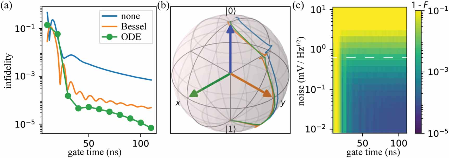
Figure 3. (a) Simulated average gate infidelity  of a swap-class gate as a function of pulse length tg
using no dynamic pulse shaping (blue), dynamic pulse shaping based on Bessel functions equation (72) (orange), and dynamic pulse shaping based on a ODE approximation of equation (69) (green). The simulation using ODE was performed with Mathematica. (b) Trajectories of the optimized pulse shapes for a
of a swap-class gate as a function of pulse length tg
using no dynamic pulse shaping (blue), dynamic pulse shaping based on Bessel functions equation (72) (orange), and dynamic pulse shaping based on a ODE approximation of equation (69) (green). The simulation using ODE was performed with Mathematica. (b) Trajectories of the optimized pulse shapes for a  projected on the Bloch sphere. Dynamic pulse shaping based on the ODE approximation gives rise to a high fidelity state flip. (c) Simulated gate infidelity
  as a function of pulse length tg
and charge noise acting on the virtual voltage considering
as a function of pulse length tg
and charge noise acting on the virtual voltage considering  with amplitude A using a Hann window and dynamic pulse shaping based on Bessel functions. The dashed line highlights the value of charge noise of the virtual voltage extracted in [32]. Single-qubit noise is added as quasi-static fluctuations with amplitudes taken from [32].
Download figure:
Standard image High-resolution imageThe swap-class is directly (linear) susceptible to low-frequency noise coupling in via the exchange interaction J. Additionally, both discussed implementations have in common that they require careful calibration to compensate for the adiabatic phase acquisition from exchange, making them (at least) equally susceptible to low-frequency charge noise as the conventional cz gate. Figure 4 compares the infidelity of the different two-qubit gate implementations discussed in this paper. It is clearly visible that the cz gate always outperforms the swap-class gate. The lower fidelity of the swap gate is due to the overall larger conditional phase picked up,  .
.

Figure 4. Simulated infidelity  of the cz gate, iswap gate, and single-qubit
  gates on qubit Q1 and Q2 as a function of charge noise acting on the virtual voltage considering
  with amplitude A. All gate times are
  . The dashed line highlights the value of charge noise of the virtual voltage extracted in [32]. Single-qubit noise is added as quasi-static fluctuations with amplitudes taken from [32].
Download figure:
Standard image High-resolution image
5. Conclusion
In this work, we have presented a framework which allows us to characterize unitary errors and suppress these errors for various basic gate operations for spin qubits. Unitary errors mostly arise due to violations of approximations such as the rotating wave approximation, larger system sizes in the form of crosstalk, and non-linear transfer functions of the input signal. Our numerical simulations show, that for state-of-the-art experiments, unitary errors can indeed be the limiting factor.
Explicitly, we used our framework to obtain optimized pulse shapes for resonantly driven single-qubit gates and exchange-based dc or ac gates on single-spin qubits. These techniques have been successfully implemented and enabled a two-qubit cz gate with fidelity  [32]. We have also shown that the optimized static pulse shapes for single-qubit gates and cz two-qubit gates are identical and depend solely on the qubit frequency separation. This possibly allows for a direct on-chip integration of the control electronics with little memory requirements. The transformation of the signal to compensate for the exponential relationship between voltage and exchange interaction is possible using efficient digital algorithms or an analogue logarithmic element.
Our framework and all presented optimized pulse shapes are directly applicable to different platforms. To suppress coherent errors even further, higher-order Magnus expansion terms can be considered [43]. In our formalism this would correspond to not only minimizing the spectral density but also minimizing higher correlations such as the bi-spectrum or multi-spectrum.
While in this work we focused on improving the performance of operations with respect to coherent errors, the formalism can also be extended to account for incoherent errors [58]. We can think of two steps how this can be achieved. First, we can either extend our formalism to describing the time dynamics in terms of a propagator based on the Liouville superoperator instead of unitary operations [57]. Alternatively, to account for low-frequency noise, we can combine our framework with the SCQC formalism introduced in [38].
Acknowledgments
The authors greatly acknowledge the contributions of S de Snoo and U Güngördü to the manuscript. We thank all members of the Veldhorst and Vandersypen group, M Mehmandoost, D Zeuch, V Evangelos, and Vincent Bejach for inspiring and constructive discussion. M R-R acknowledges support from NWO under Veni Grant (VI.Veni.212.223). This research was sponsored by the European Union's Horizon 2020 research and innovation program (QLSI Grant No. 951852) and the Army Research Office (ARO) under Grant Numbers W911NF-17-1-0274, W911NF-12-1-0607 and W911NF-22-S-0006. The views and conclusions contained in this document are those of the authors and should not be interpreted as representing the official policies, either expressed or implied, of the ARO or the US Government. The US Government is authorized to reproduce and distribute reprints for government purposes notwithstanding any copyright notation herein.
Data availability statement
The data that support the findings of this study are openly available at the following URL/DOI: https://doi.org/10.5281/zenodo.7341187.
Appendix A: Modeling the exchange interaction
Equation (37) of the main text is an approximation of the spin-dynamics in the low-energy subspace considering a single fermion in the left and right quantum dots,  charge configuration, in the presence of small spin-orbit interaction [94, 95]. The origin of the spin–orbit interaction (SOI) may arise from intrinsic properties [96] or artificial created through the deployment of micromagnets [97]. Without (with negligible) SOI, the low-energy dynamics of the spin can be derived starting from a Hubbard model with spin-conserving tunneling elements using a Schrieffer–Wolff approximation. Due to the Pauli exclusion principle, the spin state of a doubly occupied orbital state is always a spin singlet. Therefore, in the
  configuration only the singlet state,
  , can hybridize and be lowered in energy. Consequently, the exchange interaction can be written as


The dynamics of the (isotropic) exchange interaction is thus limited to the singlet-state. In the presence of a difference in qubit resonance frequencies  , the states
  and
and  are energetically separated, thus coupling the singlet with the triplet
  state.
The amplitude of the exchange interaction J is a non-linear function of an applied (virtual) barrier voltage vB . In most experiments the exchange interaction can be modeled as an exponential function [98–100]


Other experiments [10, 31], further indicate a saturation for large exchange values, thus, the upper expression (A.4) can be seen as an approximation for  . A more general expression considering saturation reads [10]

Here α is the leverarm, voff is an offset which is set by the residual exchange interaction  , and Jsat describes the saturation value of the exchange interaction when the two electrons are strongly hybridized. In practice, Jsat can be motivated to be the singlet-triplet splitting or exchange splitting for a merged double quantum dot.
The presence of a valley degree of freedom [101, 102] affects the exchange interaction J as well as the frequency difference  . In lowest-order perturbation theory, we find


where  and
and  are the respective valley splitting and valley phase of dot i. Plugging in realistic parameters
  ,
,  ,
,  MHz, and
  we find
  . On contrast, a finite valley phase difference significantly suppresses the exchange interaction [103]. For our theoretical simulations, the valley phase becomes only problematic once it changes during the pulse, e.g. due to the deformation of the wave-functions as a function of applied voltages. Since the dc and ac pulsed two-qubit gates are adiabatic with respect to the qubit frequencies
  and in most devices also with respect to the valley splitting EV
, the gates are only slightly affected by the presence of the valley degree of freedom. However, simulations of the valley phase require microscopic computations, which are not part of this paper. Therefore, we assume a constant valley phase difference, which we factor out. A last remark, both correction factors are unimportant in an experimental realization for the here discussed gates since this renormalization is already accounted for during the calibration process of the qubit energy difference and the spin exchange strength.
and in most devices also with respect to the valley splitting EV
, the gates are only slightly affected by the presence of the valley degree of freedom. However, simulations of the valley phase require microscopic computations, which are not part of this paper. Therefore, we assume a constant valley phase difference, which we factor out. A last remark, both correction factors are unimportant in an experimental realization for the here discussed gates since this renormalization is already accounted for during the calibration process of the qubit energy difference and the spin exchange strength.
In the presence of spin-orbit interaction, spin non-conserving tunneling is allowed, which gives rise to an isotropic exchange interaction [26, 104]

where  is the exchange tensor. Therefore, the dynamics of the exchange interaction is no longer limited to the
  subspace. Additionally, in the presence of SOI the quantization axis of the spins in the different quantum dots may change, thus giving rise to an additional channel that can couple the
  state with the polarized
  and
and  states. Note, that this situation may also arise for electron systems with micromagnets designed to enhance SOI [105, 106]. However, most results from this paper can still be applied to platforms with small to medium strength SOI, such as planar electron qubits in silicon and hole qubits [16], as long as a sufficiently strong external magnetic field is applied to suppress the unwanted dynamics.
Appendix B: Generalized rotating wave approximation
Although other approaches based either on the Magnus expansion [107] or Floquet engineering [108] or numerical methods [109] allow finding control pulses for a strongly driven qubit system, we find the 'exact' rotating wave approximation described in [79] to be most practical to be incorporate in non-linear situations. The effective Hamiltonian is then given by [79]

where ![$[A,B] = AB-BA$](https://content.cld.iop.org/journals/2058-9565/8/4/045025/revision2/qstacf786ieqn256.gif) denotes the commutator and
denotes the commutator and  is the time derivative. An important remark is, that HRF and
  are assumed to be either constant or periodic in the time interval
  The first line in equation (B.1) is the conventional rotating wave approximation. The second line addresses corrections due to the time-dependence of signals, such as envelopes of the applied signals. The last line includes the first order corrections of the rotating wave approximation, such as the Bloch–Siegert shift.
Appendix C: Explicit expressions for all Hamiltonians and error channels from section III
Below we show the explicit expressions for the total, ideal and erroneous Hamiltonian for the three applications discussed in section 3. Following our framework, the dominant error decomposition operators Ok
can be found from the eigenstates of the dynamic invariant at t = 0. Since in all discussed cases ![$[H_\text{ideal}(t),H_\text{ideal}(t^{\prime})] = 0$](https://content.cld.iop.org/journals/2058-9565/8/4/045025/revision2/qstacf786ieqn260.gif) , the eigenstates of Hideal can be used instead.
, the eigenstates of Hideal can be used instead.
C.1. Explicit form of the Hamiltonian and error channels for single-qubit gates
Plugging in  into equation (39) we get


The corresponding error channels follow from  with
with  , where
  are eigenstates of equation (C.2). As Hamiltonian (C.1) describes an uncoupled two-qubit system, the dynamics of each qubit can be treated independently, reducing the number of non-zero channels to two per qubit. The dynamics of qubit 1 and qubit 2 are described by a x-rotation and z-rotation that leads to the following error channels


C.2. Explicit form of the Hamiltonian and error channel for two-qubit cz gate
Plugging in  into equation (38) and diagonalizing we get the Hamiltonians


The corresponding error channels follows from  with
with  , where
  are eigenstates of equation (C.7). Hamiltonian (C.6) can be effectively reduced to a single-qubit system in the space spanned by the odd parity states
  (see appendix A). In this subspace, equation (C.7) describes a z-rotation, giving rise to

where the tilde labels the instantaneous eigenstates.
C.3. Explicit form of the Hamiltonian and error channel for two-qubit resonant swap gate
For the resonant swap gate the Hamiltonians are


The corresponding error channels follows from  with
with  , where
  are eigenstates of equation (C.11). Hamiltonian (C.10) can be effectively reduced to a single-qubit system in the space spanned by the odd parity states
  (see appendix A). In this subspace, equation (C.11) describes a x-rotation, giving rise to

where the tilde labels the instantaneous eigenstates.
Appendix D: Derivation of the optimized pulse shape for cz-gate for small Zeeman differences
For  the approximation
  fails and the optimized pulse shape condition equation (34) is given by


Here, we have combined the differentials  from line 1 to 2 and plugged in equation (55) from 2 to 3. To get the optimized pulse shape for J(s) we integrate both sides


where  is an integrated window function. Next we use the following relation

that can be obtained from equation (27) using integration by parts and enforcing  . We absorb the phase into the absolute value and arrive after some calculus at

where we redefined the constant  .
.
Appendix E: Approximating the integro-differential equation using an ordinary differential equation
Writing out equation (69) we find the integro-differential equation

The upper system is generally hard to solve. Thus, we approximate the upper expression using a series expansions in  at
at  up to first order. To arrive at an ordinary differential equation (ODE) we additionally ignore all terms under the integral which depend on θj
. A numerical check confirmed the validity, assuming reasonable smooth (with respect to
up to first order. To arrive at an ordinary differential equation (ODE) we additionally ignore all terms under the integral which depend on θj
. A numerical check confirmed the validity, assuming reasonable smooth (with respect to  ) pulse shapes.
Appendix F: Master equation solver
For all numerical simulations performed we solve the time-dependent Schrödinger equation

and compute the unitary propagator iterative according to

Here, H(t) is discretized into N segments of length  such that H(t) is constant in the time-interval
  . For the simulations of single-qubit gates in figures 1(b)–(d) we choose an external magnetic field
  and a step-size of
  . The remaining simulations involving two-qubit gates in figures 2 and 3 are performed in the rotating frame of the external magnetic field Ez
and neglecting the counter-rotating terms, the so-called rotating wave approximation (RWA). This allows us to choose the time-step
. The remaining simulations involving two-qubit gates in figures 2 and 3 are performed in the rotating frame of the external magnetic field Ez
and neglecting the counter-rotating terms, the so-called rotating wave approximation (RWA). This allows us to choose the time-step  being sufficiently small. For each simulation, we check whether the RWA holds.
In all our simulations except for the ODE in figure 3(a) (green), to emulate the realistic effect of a finite bandwidth and filtering of the control gates, we add on each input signal, amplitude and phase of barrier and drive voltage, a low-pass filter with a cut-off frequency of  . In particular, we use a Butterworth filter of order three implemented via the Scipy package [110].
All simulation parameters, if not explicitly mentioned otherwise, are taken from methods in [32] that are extracted by fitting our Hamiltonian to the measured experimental values.
For our noisy simulations we add classical fluctuations to the matrix elements of our Hamiltonian

where  are parameters describing the dynamics of the system and
  are the fluctuations of the parameter. We note that this treatment allows us to account for non-linear Hamiltonian interactions as the exchange interaction and also to include 'sweet spots', points of operation where the first order dynamics vanishes. The classical noise is added in two ways into the dynamics. Magnetic noise affecting the single spins is simulated by a quasi-static shift of the qubit resonance frequencies
  . Explicitly, we used
  with
with  and
and  from [32].
Charge noise on the electrodes is added dynamically. The time-dependent classical charge fluctuations  are described by its spectral density
  , which we use as input in our simulations. To compute time-traces of the fluctuation, we use the Fourier filtering method [84, 85] to generate time-correlated time traces obeying
  . In this method, N independent Gaussian distributed numbers are generated and associated to a segment with time
  . We then perform a discrete Fourier transformation, apply a frequency filter
  , and perform an inverse Fourier transformation. The resulting fluctuations are discretized in N segments with time
  such that
  is constant in the time interval
  . Note, that the same
  is used as above. Consequently, fluctuations which are faster than
  are truncated. The lower frequency cut-off of the discretized noise traces is given by the length of the simulation and the number of segments. To provide better comparison of the dynamics of unequal length simulations and avoid an increase in simulations length, we add static fluctuations
  to compensate for the 'missing' low-frequency components. The amount of static noise component is given by

where tsim is the length of the simulation and  is a lower-frequency cut-off and resembles the retuning cycle of an experiment.
The final superoperator of the noisy process is then constructed as follows

where  is the final unitary time evolution operator for a noise realization j and
  is the total number of noise realizations.
Appendix G: Estimation of coherent cz gate error in Mills et al
We find the following device parameter in [35] describing the cz gate; difference in qubit resonance frequency  , duration of cz gate
  using a (smoothed) rectangular pulse shape (Tukey window with λ ≈ 0) and measured
  and
and  . From equation (57) we know that the cz error probability depends solely on
  . This invariant allows us to conveniently simulate the coherent error using
  MHz (as for all other simulations in this manuscript) but using a modified pulse time
  . For the noisy simulations, we used the same noise strength as extracted from [32] (as for all other simulations in this manuscript). Fortunately, the rescaled dephasing times
  and
and  are smaller than the measured one in [32], but are still realistic values, providing an optimistic comparison.
Footnotes
- 1
Can be implemented virtually using only software phase shifts.