


ABSTRACT
Understanding the evolution of magnetic flux in the heliosphere remains an unresolved issue. The current solar minimum between cycles 23 and 24 is anomalously long, which gives rare insight into the long-term evolution of heliospheric magnetic flux when the coronal mass ejection (CME) rate and the flux emergence rate from CMEs were very low. The precipitous drop of heliospheric magnetic flux to levels lower than have ever been observed directly shows that there may be a persistent loss of open magnetic flux through disconnection, the reconnection between opposite polarity heliospheric magnetic field lines relatively near the Sun (beneath the Alfvén point). Here, we develop a model for the levels of magnetic flux in the inner heliosphere balancing new flux injected by CMEs, flux lost through disconnection, and closed flux lost through interchange reconnection near the Sun. This magnetic flux balance is a fundamental property that regulates the plasma and radiation environment of our solar system.
Export citation and abstract BibTeX RIS
1. INTRODUCTION AND BACKGROUND
During solar maximum the levels of heliospheric magnetic flux are seen to approximately double relative to their solar minimum levels (Wang et al. 2000; Connick et al. 2009). Owens & Crooker (2006) and Owens et al. (2008) argue that coronal mass ejections (CMEs) inject a new closed magnetic flux, the majority of which undergoes interchange reconnection with pre-existing heliospheric magnetic flux within 30–50 days after injection. This interchange reconnection process moves the footpoints of the associated pre-existing heliospheric magnetic field lines and leads to the loss of CME-associated magnetic flux. The CME-associated magnetic flux temporarily adds to the magnetic flux of the inner heliosphere and raises the level of the magnetic flux near solar maximum when CMEs are most frequent.
There is a well-defined relationship between the magnitude of the magnetic field observed at 1 AU and the rate that CMEs are ejected by the Sun (Owens et al. 2008). For CME rates of 0.5 day−1 to 1.5 day−1, there is a roughly linear relationship between the field strength and the CME rate. A floor in the magnetic field strength is derived by projecting the linear relationship down to a CME rate of zero. Originally, Owens et al. (2008) found a floor of 4.0 ± 0.3 nT, and a more recent revised analysis (Crooker & Owens 2010) shows a floor of ∼3.7 nT.
The concept of a floor in the heliospheric magnetic flux and a time-varying component injected from CMEs is consistent with the model of Zhao et al. (2009) in which the solar wind is divided into three components: non-transient solar wind from coronal holes (CHW), non-transient solar wind that originates from outside coronal holes (NCHW), and solar wind associated with transient interplanetary coronal mass ejections (ICMEs). The ICME-associated wind creates a "streamer-stalk" region surrounding the heliospheric current sheet. The streamer-stalk region is wider at solar maximum when CMEs are more frequent. The heliospheric magnetic flux in CHW and NCHW cannot penetrate into the base of the streamer-stalk region. Therefore, the portion of the heliospheric magnetic flux in CHW and NCHW is more likely to be conserved. Hence, Zhao et al. (2009) provide a physical basis for a floor in the heliospheric magnetic flux. Since all disconnection occurs at the current sheet, the magnetic flux injected by ICMEs that straddles the current sheet (the streamer-stalk region) prevents the magnetic flux outside the streamer-stalk region from approaching the current sheet and undergoing disconnection.
The magnetic flux in the heliosphere can be estimated using the radial magnetic field strength, Br as a proxy:

This definition makes sense only if we assume that the radial field strength is uniform in longitude and latitude at radial distance R. Of course, this is not the case, particularly on small scales, and, as a result, estimating the total flux requires analysis. Owens et al. (2008) explore the method of estimating the total heliospheric magnetic flux from single-point in situ measurements and compare flux estimates from different spacecraft. They use 1 hr averages of Br in time series and form ensemble averages over a Carrington rotation (∼26 days). The average over a Carrington rotation generally smooths out variations in longitude. The latitudinal invariance of the magnetic flux has been reported from Ulysses observations (Smith & Balogh 2003; Lockwood et al. 2004). Owens et al. (2008) conclude that single-point measurements are adequate proxies for the total heliospheric magnetic flux, although care must be taken when comparing flux estimates from data taken at different distances from the Sun.
Other methods of deducing open (and toroidal) magnetic flux were introduced and used by McComas et al. (1992), Bieber & Rust (1995), Smith & Phillips (1997), and Connick et al. (2009). These methods allow decomposition of the magnetic flux into a component along the Parker spiral, two components perpendicular to the Parker spiral resulting in toroidal flux, and the flux of spiral-aligned field that pierces a Sun-centered surface.
Recent observations of the heliospheric magnetic flux show that it has continued to decrease precipitously (Lockwood et al. 2009a, 2009b; Connick et al. 2010). This drop in the magnetic flux is associated with the weakening in the Sun's polar fields, currently ∼40% weaker than the three sunspot minima previous to the current minimum between cycles 23 and 24 Wang (2009). This weakening in the magnetic flux is also associated with ∼20% shrinkage in the polar coronal-hole areas and a reduction in the solar wind power and mass flux (McComas et al. 2008; Schwadron & McComas 2008). Here, we develop a model that includes the loss of heliospheric magnetic flux through disconnection and show its importance in addition to the introduction of new flux by CMEs.
2. MODEL FOR SOURCES AND LOSSES OF HELIOSPHERIC MAGNETIC FLUX
CMEs provide sources of magnetic flux to the heliosphere. The new closed magnetic flux from CMEs is transformed in three ways (Figure 1). Interchange reconnection (top panel) between the new closed magnetic flux from CMEs and surrounding field lines open to the heliosphere leads to the destruction of closed flux, the displacement of the footpoint of the pre-existing field line, and the extension of the coronal hole (or creation of new coronal holes). The interchange reconnection process is favored if the CME orientation opposes that of the large-scale magnetic flux. The effects of the interchange reconnection process lead to the reversal of the large-scale heliospheric magnetic field through solar maximum (Owens et al. 2007; Schwadron et al. 2008). Clearly, CMEs are transient phenomena, introducing new magnetic flux that is not near a minimum energy potential state. Interchange reconnection allows removal of non-potential field and a means to return nearer to the minimum energy state.
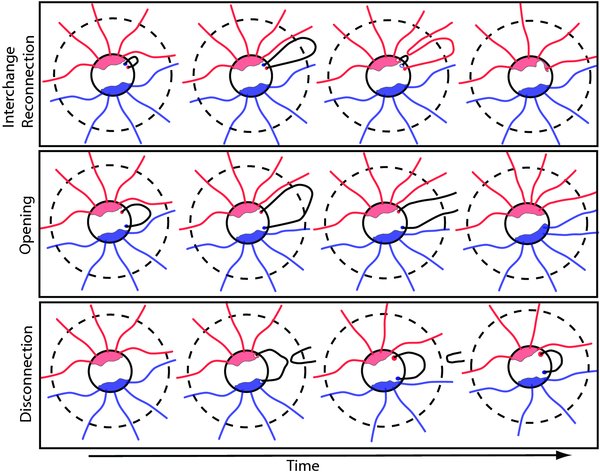
Figure 1. Three processes considered in the magnetic flux balance of the heliosphere. Top panel: interchange reconnection destroys closed magnetic flux, displaces pre-existing field lines open to the heliosphere, and leads to distortions in the coronal hole. The interchange reconnection process does not change the levels of pre-existing heliospheric magnetic flux, but the presence of closed CME-associated flux raises the net flux in the heliosphere. Middle panel: CMEs can eject loops, which may add to the heliospheric flux if the loops have the same orientation as the large-scale magnetic flux. The opening process increases the area of coronal holes. Bottom panel: disconnection leads to the removal of pre-existing magnetic flux open to the heliosphere and to the reduction of coronal holes. The dashed line in these illustrations indicates the Alfvén surface (typically 10–15 Rs; not to scale) above which magnetic reconnection can have no long-term effect on the reconfiguration heliospheric flux.
Download figure:
Standard image High-resolution imageLong-lived loops (Figure 1, middle panel) migrate into configurations closer to a minimum energy state. Eruptive processes drag these long-lived closed structures into the solar wind where they are unlikely to be destroyed because they have the same orientation as the pre-existing magnetic flux open to the heliosphere. Instead of being destroyed, these closed structures continue to be dragged out by the solar wind and become a component of the heliospheric magnetic field indistinguishable from the pre-existing heliospheric flux.
In the destruction of heliospheric magnetic flux through disconnection (bottom panel), open magnetic flux reconnects beneath the Alfvén surface (where the solar wind speed equals the Alfvén speed), causing an inverted U-shaped structure that is ejected from the heliosphere by the solar wind. The two oppositely oriented field structures are therefore converted into a closed loop back at the Sun, resulting in a decrease in the size of coronal holes. In all three of these cases, reconnection must occur beneath the Alfvén surface to cause any long-term reconfiguration of the magnetic flux.
Kinematic effects may increase the observed heliospheric flux with distance from the Sun. Owens et al. (2008) showed that Φ is not constant but increases with r. This effect may be explained by the longitudinal solar wind flow structure within the streamer belt (Lockwood et al. 2009a; Lockwood & Owens 2009) and may be part of the reason that potential field source surface (PFSS) models predict levels of the heliospheric flux lower than observed in situ near 1 AU (Lockwood et al. 2009a).
We introduce a simple model for the sources and losses of heliospheric magnetic flux. The model follows from similar pre-existing models (Owens & Crooker 2006; Owens et al. 2008), however, we include several new terms. There is a source term for closed magnetic flux: ejecta effectively create new closed magnetic flux by dragging out field structures from the Sun that are, topologically, elongated loops. We take the flux content of a typical CME, ϕCME ∼ 1 × 10¹³ Wb (Owens 2008). However, a large fraction, D ∼ 1/2, of this flux opens as the CME launches from the Sun (Owens & Crooker 2006). So the closed flux created by an individual CME is (1 − D)ϕCME. The other factor that enters the source term for closed ejecta-associated flux is the frequency, f(t), of CME ejection, which depends on time, t, varying typically from flo∼ 0.5 day−1 near solar minimum to fhi ∼ 3 day−1 near solar maximum (Owens et al. 2008). In principle, one can create a constrained function f(t) based on direct observations of CMEs. Here, for time periods prior to 2006, we use a simple representation of ![$f(t < t_{\rm min}) = f_{\rm{lo}} + (f_{\rm hi} - f_{\rm lo}) \sin ^2[\omega (t - t_{\rm min})]$](https://content.cld.iop.org/journals/2041-8205/722/2/L132/revision1/apjl352484ieqn1.gif) , where the sin2[ω(t − tmin)] arises from solar cycle variation of the CME rate, and tmin ∼ 2006 is the time of the last nominal solar minimum. The term ω = π/11 years−1 represents the frequency of the solar cycle. For the time period following 2006 to present (2010 March), the Sun has remained anomalously quiet, and we take f(t>tmin) = flo. Combining all of this, the source term for closed magnetic flux is simply Sc(t) = f(t)(1 − D)ϕCME(t).
, where the sin2[ω(t − tmin)] arises from solar cycle variation of the CME rate, and tmin ∼ 2006 is the time of the last nominal solar minimum. The term ω = π/11 years−1 represents the frequency of the solar cycle. For the time period following 2006 to present (2010 March), the Sun has remained anomalously quiet, and we take f(t>tmin) = flo. Combining all of this, the source term for closed magnetic flux is simply Sc(t) = f(t)(1 − D)ϕCME(t).
There are three losses of closed ejecta-associated magnetic flux. First, as in previous models, closed flux undergoes interchange reconnection on timescale, τic, with pre-existing heliospheric flux, removing the reconnected ejecta-associated flux. Owens et al. (2008) take an exponential decay of the ejecta-associated magnetic flux created by an ICMEs, ϕc ∝ (1 − D)ϕCMEexp(−t/τic), where τic is the timescale for closed flux loss through interchange reconnection. This exponential decay is equivalent to introducing a loss term of ejecta-associated magnetic flux, −Φej/τic, on a characteristic timescale of τic, where τic ∼ 30–50 days (Owens et al. 2008).
The second loss mechanism for ejecta-associated magnetic flux is opening (middle panel, Figure 1). After ejection, the footpoints of ejecta-associated field lines are relatively near active regions, or regions of mixed polarity where the probability of reconnection is high. Eventually, after the ejecta has propagated far from the Sun, the only surviving flux must migrate into regions of uniform polarity, e.g., coronal holes. Eventually the topologically closed loop connected through the ejection will propagate through the inner solar system. For all practical purposes, then, this small surviving ejecta-associated magnetic flux becomes indistinguishable from the surrounding heliospheric magnetic flux. The "opening time," τo, must be much larger than the interchange reconnection timescale, τic. On a ∼2 year timescale, we might expect meridional motions (∼10 m s−1) to move some fraction of ejecta-associated flux footpoints into coronal holes (e.g., over a year at 10 m s−1, a photospheric element moves ∼600,000 km, which is roughly equal to a solar radius). Diffusive motions of footpoints (Fisk & Schwadron 2001) could also easily account for their passage into coronal holes on timescales of around two years. In the opening process, there is no net loss of flux to the heliosphere: the loss of ejecta-associated magnetic flux is balanced by the gain of heliospheric flux.
The final loss mechanism is disconnection (McComas et al. 1992; bottom panel, Figure 1). Connick et al. (2010) consider this in the context of reconnection between heliospheric magnetic field lines of opposite polarity beneath the Alfvén point. The result is the creation of a field line that does not connect to the Sun and is subsequently moved by the solar wind out of the system. The objection raised to this as a process for discarding flux is that we would require the observation of significant numbers of electron dropouts, which are rarely observed. However, contrary to previous expectations, Owens & Crooker (2007) find that if the closed flux added to the heliosphere by CMEs is balanced by disconnection elsewhere, then the occurrence of electron dropouts at 1 AU would be rare, and beneath current observational limits. Due to the expected rarity of disconnection events, the timescale, τd, for the loss magnetic flux process is very difficult to derive.
Owens et al. (2008) and Crooker & Owens (2010) have shown based on the almost linear correlation between the magnetic field strength and the CME rate that there may be a floor in the level of heliospheric magnetic flux. Such a floor has also been suggested (Wang et al. 2000) on the basis that the solar wind provides sufficient pressure to drag out at least some of the field lines from the low corona. If there exists a floor in the heliospheric flux, then the rate of flux loss due to disconnection must be relative to the floor, Φflr.
With the source of magnetic flux from CMEs and the losses of ejecta-associated flux from interchange reconnection, opening, and disconnection, we find the following equation for the balance of closed magnetic flux,
For magnetic flux not associated with ejecta, Φ0, we must take into account the source of flux from the opening of ejecta-associated flux and the loss through disconnection,
From the sum of the two equations, we find that the total flux in the heliosphere is a balance between disconnection and the source of ejecta-associated flux, which can be lost through interchange reconnection:
The integral solution for the ejecta-associated and non-ejecta-associated heliospheric flux is
where the characteristic loss-time of closed flux is
Given the assumed form of the CME frequency, we find the following analytic solutions to these integrals. For t < t0 we find
For t ⩾ t0 we find
Figure 2 shows a solution for the ejecta- and non-ejecta-associated magnetic flux expressed in terms of field magnitude at 1 AU, assuming a 45° Parker spiral ( where R1 is 1 AU). We have also taken ϕCME = 1 × 10¹³ Wb, D = 1/2, τic = 40 days, τo = 2.5 years, τd = 7.4 years, flo = 0.5 day−1, fhi = 3 day−1 and Φflr = 0. We find the periodic behavior of the magnetic flux as it rises and falls in response to the rate of CMEs magnetic flux. In addition, we see the recent falloff in the magnetic field strength due to disconnection of the magnetic flux in the prolonged solar minimum.
Figure 2. Evolution of the ejecta-associated magnetic flux, non-ejecta-associated heliospheric magnetic flux, and total magnetic flux over the cycle shows both the periodic buildup of magnetic flux near solar maximum due to CME ejection and the steady decay of heliospheric magnetic flux during the extended solar minimum between cycles 23 and 24. We take a 45° Parker spiral ( , where R1 is 1 AU). We also take ϕCME = 1 × 10¹³ Wb, D = 1/2, τic = 40 days, τo = 2.5 years, τd = 7.4 years, flo = 0.5 day−1, fhi = 3 day−1, and Φflr = 0.
Download figure:
Standard image High-resolution imageFigure 3 shows another solution like the one in Figure 2 but for a non-zero flux floor, Φflr = 4 × 10¹⁴ Wb, consistent with a field strength at 1 AU of 2 nT. We have used the same parameters as those used in Figure 1, except the disconnection time is shorter, τd = 4.4 years.
Figure 3. Evolution of magnetic flux for a non-zero floor in the magnetic flux (Φflr = 4 × 10¹⁴ Wb consistent with a field strength at 1 AU of 2 nT) and a reduced disconnection time, τd = 4.4 years. All other parameters are the same as in Figure 2.
Download figure:
Standard image High-resolution image
Although we explored a variety of different parameters, it is difficult to increase the floor in the magnetic field above the Φflr = 4 × 10¹⁴ Wb and still derive results in agreement with observations. This suggests a floor in the heliospheric flux ⩽4 × 10¹⁴ Wb.
3. DISCUSSION
The evolution of the magnetic field in the heliosphere in the anomalously long solar minimum between cycles 23 and 24 shows the weakest magnetic field strengths so far observed during the space age. These observations provide strong evidence that the heliospheric magnetic field is disconnected from the Sun at a slow rate (Connick et al. 2010). Here, we develop a model for the evolution of heliospheric magnetic flux including the sources of closed flux from CMEs and the rate balance between flux disconnection, opening and interchange reconnection. The model can account both for the periodic buildup of heliospheric magnetic flux near solar maximum and the decay of heliospheric magnetic flux through the disconnection during the extended solar minimum.
Our study, while a preliminary comparison to observations, shows that the floor in the heliospheric magnetic field may be lower than previously thought. The suggestion of a much lower magnetic flux floor is consistent with other studies showing a long-term drift in large-scale solar flux (Lockwood & Stamper 1999). Further, Lockwood et al. (2009b) argue that there was never a justification for a floor in the heliospheric magnetic field.
Schwadron & McComas (2008) show that the solar wind power and mass flux scale with and are likely controlled by the magnetic flux of the heliosphere. This implies that whatever controls the level of magnetic flux in the heliosphere also regulates the mass loss of our star, and the net power of our solar wind, which, in turn, helps to control the size of our heliosphere. The amount of magnetic flux of the heliosphere is also fundamental for regulating the modulation of galactic cosmic rays, which in turn influences the radiation environment of the inner heliosphere. Presumably, other magnetic stars also must balance the magnetic flux from transient stellar mass ejections, interchange reconnection, opening and disconnection. Therefore, understanding the magnetic flux balance of the heliosphere has important implications for understanding other stars and their associated astrospheres.
Thus, our model shows that the magnetic flux of the heliosphere results from a balance between the new magnetic flux injected by CMEs, the loss of closed magnetic flux through interchange reconnection, the conversion of closed to open magnetic flux, and the loss of magnetic flux through disconnection. This magnetic flux balance is a fundamental property that regulates the plasma and radiation environment of our solar system.
D.E.C. and C.W.S. are funded by Caltech subcontract 44A-1062037 to the University of New Hampshire in support of the ACE/MAG instrument. N.A.S. is funded by the NASA EMMREM project, grant NNX07AC14G.