

Abstract
We apply climate attribution techniques to sea surface temperature time series from five regional North Pacific ecosystems to track the growth in human influence on ocean temperatures over the past seven decades (1950–2022). Using Bayesian estimates of the Fraction of Attributable Risk (FAR) and Risk Ratio (RR) derived from 23 global climate models, we show that human influence on regional ocean temperatures could first be detected in the 1970s and grew until 2014–2020 temperatures showed overwhelming evidence of human contribution. For the entire North Pacific, FAR and RR values show that temperatures have reached levels that were likely impossible in the preindustrial climate, indicating that the question of attribution is already obsolete at the basin scale. Regional results indicate the strongest evidence for human influence in the northernmost ecosystems (Eastern Bering Sea and Gulf of Alaska), though all regions showed FAR values > 0.98 for at least one year. Extreme regional SST values that were expected every 1000–10 000 years in the preindustrial climate are expected every 5–40 years in the current climate. We use the Gulf of Alaska sockeye salmon fishery to show how attribution time series may be used to contextualize the impacts of human-induced ocean warming on ecosystem services. We link negative warming effects on sockeye fishery catches to increasing human influence on regional temperatures (increasing FAR values), and we find that sockeye salmon migrating to sea in years with the strongest evidence for human effects on temperature (FAR ⩾ 0.98) produce catches 1.4 standard deviations below the long-term log mean. Attribution time series may be helpful indicators for better defining the human role in observed climate change impacts, and may thus help researchers, managers, and stakeholders to better understand and plan for the effects of climate change.
Export citation and abstract BibTeX RIS

Original content from this work may be used under the terms of the Creative Commons Attribution 4.0 license. Any further distribution of this work must maintain attribution to the author(s) and the title of the work, journal citation and DOI.
1. Introduction
Extreme event attribution (EEA) has been important for building recognition of the impacts of human-induced climate change, as it provides a way to quantify the link between human activity and impacts such as heatwaves, fires, and floods [1–4]. EEA provides a useful context for understanding climate change that may be lacking from data on primary climate variables alone, such as temperature [5]. And EEA has been proposed as a potentially valuable tool for adaptation planning, either within the academic community or for the broader public [5–7]. However, extreme events that are the focus of EEA are by definition individual events, as the technique was developed to answer the question of whether a particular climate event, usually one with severe health or economic consequences, could be ascribed to human activities. One shortcoming of this focus on individual events is the problem of which events to select for analysis, which may open attribution studies to perceptions of bias [5, 8]. And EEA does not provide a temporal context for the growth of human influence on the climate. This temporal context can be critical for effective adaptation decision-making. For instance, incremental changes over time may create extreme impacts on ecosystem services [9, 10], but stakeholders may have more difficulty in recognizining the consequences of incremental change than extreme events [11, 12]. Expanding EEA into a time series setting, allowing for statements about the changes in human influence on a given system over time, would allow a broader set of questions around climate change adaptation and mitigation to be addressed.
Ocean warming has profound consequences for fisheries production and other critical ecosystem services globally [13, 14], and new approaches for contextualizing ocean warming are important for successful adaptation planning [5, 15, 16]. For instance, relating declining productivity of fish stocks to increasing human influence over regional temperatures may provide information about declining fisheries sustainability, a critical adaptation challenge for stakeholders [17]. Here, we apply EEA techniques to time series of sea surface temperature (SST) observations for the North Pacific basin and five regional ecosystems during 1950–2022, rather than to an individual extreme SST event. Our overall objective is to use attribution time series to measure changes in human influence on marine climate over time as an approach for recognizing and understanding the impacts of human-induced climate change on ecosystem services. Our specific goals are to: (1) build attribution time series to document the evolution of human influence on North Pacific and regional SST; (2) evaluate changes in the expected return time for extreme SST events (the warmest conditions observed to date) in historical, current, and decadal-scale future climates as an additional approach for illustrating the speed and magnitude of climate change effects in the North Pacific; and (3) demonstrate the potential of attribution statistics for contextualizing climate change and informing adaptation decision-making by comparing outcomes for an ecosystem service (fisheries catch) under different degrees of human influence on the climate, and by providing estimates of climate risk to that service during historical, current, and next-decade climate states.
2. Methods
2.1. Attribution time series
We use the Fraction of Attributable Risk (FAR; [18–20]) to attribute the human contribution to observed SST anomalies:
The preindustrial probability is the likelihood that a given event might occur in a counterfactual world without human influence on the climate, while the current probability is the likelihood for the same event in the factual world with human influences [21]. Using the ratio of these probabilities, FAR gives an estimate of the proportion of risk for a class of event (SST anomalies ⩾ observed) that can be assigned to human influence. We also calculate the related Risk Ratio (RR) statistic [21], the ratio of risk for the same class of events with and without human activities:

A RR value of 10, for example, is evidence that a given class of event is ten times more likely to occur due to human influence on the climate.
We calculated FAR and RR values for ERSSTv5 SST observations [22] from 1950–2022 averaged over six areas: the North Pacific basin poleward of 20° N, and five northeast Pacific regional ecosystems (Eastern Bering Sea, Gulf of Alaska, British Columbia Coast, and Northern and Southern California Current; figure 1). Our regional focus is motivated by the scale over which fisheries are typically managed.
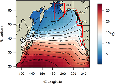
Figure 1. Study area: North Pacific basin and five regional ecosystems, with 1854–2022 mean sea surface temperature (SST) plotted. EBS = Eastern Bering Sea, GOA = Gulf of Alaska, BCC = British Columbia Coast, NCC = Northern California Current, SCC = Southern California Current.
Download figure:
Standard image High-resolution imageWe calculated FAR and RR from individual ensemble members for 23 Coupled Model Intercomparison Project Phase 6 (CMIP6) models ([23]; table 1), using normalized SST anomalies relative to the pre-1950 time series (1854–1949 for observations, 1850–1949 for CMIP6). This reference period was selected to be long enough to summarize a wide range of conditions related to internal variability, before the 1960s emergence of the observed anthropogenic trend in global temperature [24]. For each SST observation, preindustrial probabilities were estimated for each CMIP6 model as the proportion of SST anomalies from preindustrial runs producing anomalies as large as or greater than the observed SST anomaly. Present-day probabilities were calculated for each model using combined historical and SSP5-8.5 runs. Population dynamics for exploited fishes are affected by climate conditions at multiple life stages [25, 26], so average conditions over several years may be more important for fisheries yield than annual conditions [27]. We therefore calculate FAR for both annual and three-year running mean values of SST.
Table 1. Shared Socioeconomic Pathways (SSP) runs used for each of the 23 CMIP6 models in the study. Historical runs were used for every model.
| Model | SSP5-8.5 | SSP2-4.5 |
|---|---|---|
| ACCESS-CM2 | X | X |
| ACCESS-ESM1-5 | X | X |
| BCC-CSM2-MR | X | X |
| CAMS-CSM1-0 | X | X |
| CanESM5-CanOE | X | X |
| CanESM5 | X | X |
| CESM2-WACCM | X | X |
| CESM2 | X | X |
| CIESM | X | X |
| CMCC-CM2-SR5 | X | X |
| CMCC-ESM2 | X | X |
| CNRM-CM6-1 | X | |
| EC-Earth3-CC | X | |
| GISS-E2-1-G | X | X |
| HadGEM3-GC31-LL | X | X |
| HadGEM3-GC31-MM | X | |
| INM-CM4-8 | X | X |
| INM-CM5-0 | X | X |
| MIROC-ES2L | X | X |
| MIROC6 | X | X |
| NorESM2-LM | X | X |
| NorESM2-MM | X | X |
| UKESM1-0-LL | X | X |
Model bias and non-independence may make the equal weighting of climate models suboptimal [28], so we weighted CMIP6 models to reward model skill and independence [29, 30]. For each model i, the weight wi is calculated as:
where Di
is the distance of model i to the observations (i.e. the difference between model i and observations in scaled units of the weighting variable), Sij
is the distance of model i to model j, M is the total number of models, and σD
and σS
are the shape variables; the numerator is the skill weight and the denominator is the independence weight. Values of σD
and σS
were selected using a perfect model setup (see
2.2. Extreme event return times
Expected return time (the inverse of annual probability) is an established approach for evaluating the likelihood of extreme climate events [31]. To evaluate the changing incidence of extreme SST events over time, we calculated the expected return time for the warmest SST observation in each region at a range of North Pacific warming levels (preindustrial, 1950 to 0.5° warming, 0.5° to 1.0° warming, 1.0° to 1.5° warming, 1.5 °C to 2.0 °C warming). The CMIP6 multi-model probability of extreme events was estimated with a weighted Bayesian regression using annual probability (proportion of annual SST anomalies ⩾ the largest observed) as the response variable, the North Pacific warming level as a categorical explanatory variable, and the model weights described above.
Timing of 0.5 °C warming increments for the North Pacific was estimated for observations using a Bayesian smoothed regression fitting year (as the response variable) to warming relative to 1854–1949 (explanatory variable). For CMIP6 models, a weighted regression of the same formulation was employed to generate a multi-model estimate, using a single weighting criterion based on skill and independence for modeling the observed warming trend (see
2.3. Contextualizing climate impacts with attribution time series
We use the Gulf of Alaska commercial sockeye salmon (Oncorhynchus nerka) fishery as a case study to show how attribution time series can contextualize the human role in observed climate change impacts on ecosystem services. Gulf of Alaska sockeye salmon support a commercial fishery with an average ex-vessel value of $64.4M USD during the last decade [32], and are an important cultural, subsistence, and recreational resource. Commercial harvest data were obtained from the Alaska Department of Fish and Game [32]. Productivity in this species (adult offspring per spawner) shows strong responses to ocean temperature at multiple life history stages, such that three-year running mean SST is a better predictor of productivity than annual SST [25, 27].
This analysis followed four steps. First, we confirmed the negative relationship between ocean warming and sockeye productivity [27] with a Bayesian regression model relating catch to three-year running mean SST, weighted by the average year of ocean entry for each harvest year (see
The natural log of catch was used as the response variable and the models also included an autocorrelated error term to account for serial dependence in catch. We limited analysis to catch years 1989–2022 in order to avoid the complexity of nonstationary SST-salmon relationships earlier in the time series [27, 33].
Bayesian models were fit using Stan 2.21.0 [34] and R 4.1.2 [35]. For all parameters, the potential scale reduction factor ( ) was less than 1.01, effective sample sizes were greater than 500, and there were no divergent transitions in the No-U-Turn-Sampler Markov chain Monte Carlo algorithm. We evaluated chain convergence and model fits graphically (e.g. with trace plots), and via posterior predictive checks [36].
3. Results
3.1. Attribution time series
Raw SST for CMIP6 models showed strong and variable bias compared with observations (
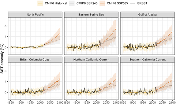
Figure 2. Modelled and observed temperature change in the North Pacific basin and five regional ecosystems: sea surface temperature (SST) anomalies (°C) relative to the pre-1950 mean for three CMIP6 runs (Historical, SSP2-4.5, SSP5-8.5) and ERSSTv5 observations. CMIP6 values are weighted multi-model mean values (lines) ± 2 weighted standard deviations (shaded ribbons).
Download figure:
Standard image High-resolution imageAll five regions, plus the overall North Pacific, have reached temperatures that can be attributed to human activities with high confidence (i.e. FAR > 0.98). In particular, North Pacific SST has effectively become fixed in an anthropogenic state, with FAR ⩾ 0.99 for three-year running mean SST since 2003, and for annual SST since 2013 (figure 3). The last years when regional SST was at levels equally likely with or without human influence (i.e. FAR 95% credible intervals that include zero) are clustered in the years following the well-described 1976/77 shift to a positive state in the Pacific Decadal Oscillation (table 2). All regional ecosystems showed FAR values > 0.98 for at least part of the 2014–2019 marine heatwaves that presented unprecedented climate perturbations to northeast Pacific ecosystems [37–39]. However, the trend and pattern in reaching these high levels of attributable risk varied among regions. Most notably, FAR estimates show a north-south gradient that is consistent with Arctic amplification of global warming. The two northernmost ecosystems have shown FAR > 0.5 (anomalies twice as likely due to human influence) for three-year running mean SST in every year since 1984 (Eastern Bering Sea) and in every year but one since 1993 (Gulf of Alaska). The strongest evidence for anthropogenic influence is seen in the northernmost region (Eastern Bering Sea), which exceeded FAR values of 0.99 for three-year running mean SST as early as 2003/2004. Annual SST FAR values for this system also exceeded 0.99 for each year from 2014 through 2020. Annual SST FAR in the Gulf of Alaska and British Columbia Coast exceeded 0.98 for at least two years since 2015, and these systems have experienced FAR > 0.99 for three-year running mean SST for five or six years since 2014. Recent FAR values were lowest for the lower latitude systems (Northern and Southern California Current), with values > 0.99 for annual SST in only one year (2015), and values > 0.99 for three-year running mean SST during 2014–2017.
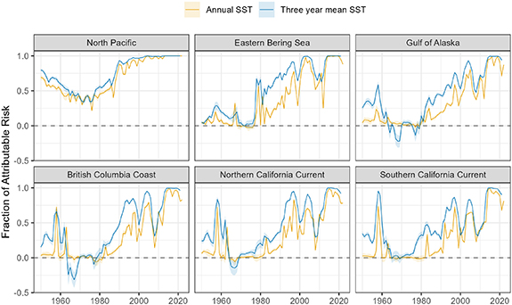
Figure 3. Attribution time series for the North Pacific Ocean and regional ecosystems: multi-model estimates of the Fraction of Attributable Risk (FAR) for annual and three-year running mean SST with 95% credible intervals, 1950-2022. Dashed horizontal line at FAR = 0 indicates temperatures that are equally likely with and without human-induced climate change.
Download figure:
Standard image High-resolution imageTable 2. Timing for the final year in each region during which FAR values for SST observations at two temporal scales (annual and three-year running mean) could not be distinguished from zero, as determined by Bayesian posteriors with 95% credible intervals that included 0.
| Region | Window | Final year |
|---|---|---|
| Eastern Bering Sea | Annual | 1982 |
| Three year mean | 1976 | |
| Gulf of Alaska | Annual | 1979 |
| Three year mean | 1981 | |
| British Columbia Coast | Annual | 1982 |
| Three year mean | 1980 | |
| Northern California Current | Annual | 1981 |
| Three year mean | 1977 | |
| Southern California Current | Annual | 1984 |
| Three year mean | 1971 |
FAR values cannot exceed one, reducing the sensitivity of this metric at high levels of human influence. RR time series provide additional information about the evolution of human influence on climate to date: annual SST in each region has reached extreme levels that are tens to hundreds of times more likely due to human activities (figure 3). The effects of spatial scale (basin vs. regional) and Arctic amplification are also illustrated by RR time series. North Pacific RR values have exceeded 105 for both annual and three-year mean SST; Eastern Bering Sea RR values have exceeded 104 (for three-year mean SST), while RR values for other regions have peak values of 102–103 (figure 4).
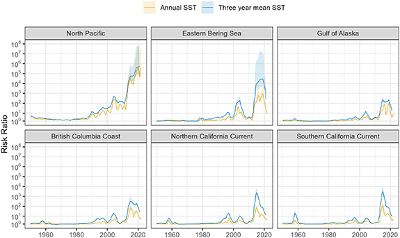
Figure 4. Attribution time series for the North Pacific Ocean and regional ecosystems: multi-model estimates of the Risk Ratio (RR) for annual and three-year running mean sea surface temperature (SST) with 95% credible intervals, 1950–2022.
Download figure:
Standard image High-resolution image3.2. Extreme event return times
We found a rapid decrease in expected return times for extreme SST values, as anomalies that were exceedingly rare have become common events (figure 5(A)). In addition, there are important regional differences that provide context for observed SST extremes in the different ecosystems. The Eastern Bering Sea has experienced the largest annual SST anomaly to date of any of the regions we consider (5.08 SD), and projected return times indicate that anomalies this large should be expected every ∼40 years in the current climate (1.0 °C–1.5 °C warming, see below). The neighboring Gulf of Alaska has experienced the smallest observed anomaly of any of the regions (2.98 SD), and anomalies this large are expected every ∼5 years in the current climate. Strong ecosystem and fisheries responses have been ascribed to warm anomalies in the two systems [39, 40], but these results suggest that stakeholders should expect repeat events to be much more common in the Gulf of Alaska than in the Bering Sea.
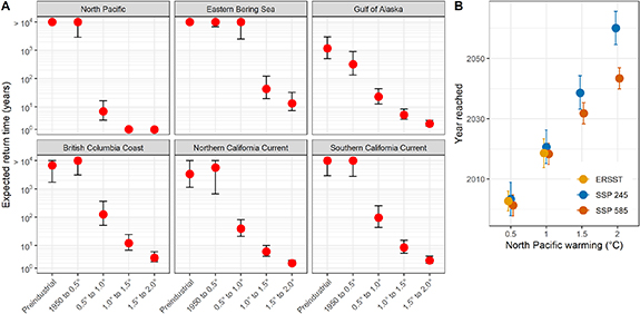
Figure 5. Historical, current, and short-term future expectations for extreme annual SST events. (A) Expected return time for warmest observed SST in each region in different climate states, defined by amount of North Pacific warming with respect to 1850-1949. (B) Estimated timing that different North Pacific warming levels have been or will be reached for observed data (ERSSTv5) and two CMIP6 emissions scenarios. Plotted data are posterior means and 95% credible intervals.
Download figure:
Standard image High-resolution imageWe found good agreement between observations and CMIP6 scenarios for the timing of 0.5 °C and 1.0 °C of warming (range of 2001–2003 and 2018–2021, respectively). The projected timing of 1.5 °C and 2.0 °C begins to diverge for the two SSP scenarios in a way that demonstrates the projected effects of mitigation on North Pacific warming (projected dates for SSP2-4.5 of 2039 and 2060 for 1.5 °C and 2.0 °C, respectively; and 2032 and 2044, respectively, for SSP5-8.5; figure 5(B)).
3.3. Contextualizing climate impacts with attribution time series
Regression of sockeye salmon catches on SST confirmed the documented negative response of the fishery to recent warming (figure 6(A)). A companion regression of catch on FAR values indicates that declines in sockeye harvests can also be statistically related to the increasing evidence for human influence on Gulf of Alaska climate (figure 6(B)). FAR values for catch years 1989–2016 varied between 0.33 and 0.91, indicating unmistakable but relatively moderate evidence for anthropogenic influence (SST values that are 1.5–11 times more likely because of human activity). For catch years 2017–2022, evidence for anthropogenic influence on temperature was much stronger (FAR = 0.98–0.99, indicating temperatures that were 60–190 times more likely due to human influence). We found a decline of 1.4SD in ln(catch) for the high-FAR years (FAR ⩾ 0.98), which corresponds to a 39% decline in raw catch relative to the 1989–2022 mean (figure 6(C)). The FAR values in the high-anthropogenic state (FAR ⩾ 0.98) correspond with a critical threshold of three-year running mean SST 2.08 SD above the pre-1950 climatology. Probability densities for three-year mean SST values at different warming increments illustrate the rapid change in the expected incidence of temperatures at or above this threshold value, and thus an estimate of changing climate risk for this fishery. Temperatures at or above the threshold were rare to uncommon events in historical climates (0% of three-year running mean SST values in the preindustrial climate, 1.4% between 1950 and 0.5 °C warming, 20% for 0.5 °C–1.0 °C of warming). But the critical threshold is close to the median value in the current climate (49% of values above the threshold for 1.0 °C–1.5 °C of warming). And the critical threshold is projected to represent cooler-than-normal conditions at 1.5 °C–2.0 °C warming (80% of values at or above the threshold; figure 6(D)).
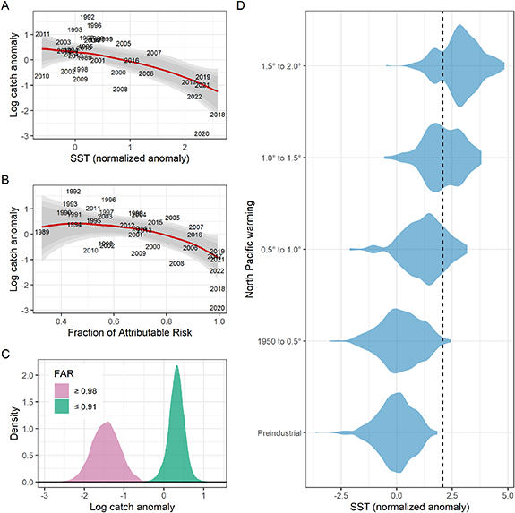
Figure 6. Context for warming effects on the Gulf of Alaska sockeye salmon commercial fishery. (A) Relationship between three-year running mean SST for each catch year, centered on year of ocean entry, and log commercial catch anomalies. (B) Relationship between the corresponding Fraction of Attributable Risk values and log commercial catch anomalies. Lines in (A), (B) are posterior means from Bayesian regression, with 80/90/95% credible intervals. (C) Fishery production (log catch anomaly) for catch years from fish experiencing moderate anthropogenic temperature effects at ocean entry (FAR ⩽ 0.91) and those experiencing more pronounced anthropogenic warming (FAR ⩾ 0.98): full posterior distributions. (D) Probability densities for three-year running mean SST values at different levels of North Pacific warming. Dashed vertical line indicates value of 2.08, (the value for 2017 in panel (A)), above which negative effects of SST on sockeye catch have been observed.
Download figure:
Standard image High-resolution image4. Discussion
The temporal evolution of climate change is often quantified with time of emergence studies, and this approach has provided important temporal context for adaptation and mitigation planning [41, 42]. The climate attribution time series presented in this study provide a complementary perspective on the evolution of human influence over North Pacific climate, based on evaluating the growing evidence for human impacts on temperature, rather than the emergence of the forced trend from the window of natural variability. While previous EEA studies have attributed post-2014 marine heatwaves in the North Pacific to human influence [31, 43–45], our results show that these extreme events are part of a persistent trend of increasing human influence on North Pacific climate that extends to the 1970s or early 1980s in every region we considered. The gradual increase in human influence documented by our attribution time series illustrates the 'shifting baseline' syndrome that may be difficult for humans to recognize, and therefore presents a particular adaptation challenge [11, 12]. In the time since FAR values could first be distinguished from zero, the proportion of risk that can be ascribed to human activities has grown from detectable to overwhelming, as indicated by RR values on the order of 101–104 at the regional scale (figure 4). These RR values indicate that recent temperatures for the entire North Pacific have reached levels that are tens of thousands of times more likely to occur due to human activities. This result is consistent with the view that contemporary surface temperatures have in many cases reached levels that were impossible under preindustrial conditions [46]. We conclude that the question of attribution has already become obsolete at the scale of the entire North Pacific.
Our results also show that the evidence for human influence on North Pacific temperatures is consistently stronger for three-year running mean SST than for annual SST values. This is an expected consequence of conducting attribution at longer temporal scales [3, 47]. But this result also suggests an important ecological insight that is gained from attribution of observation time series rather than for individual events. The multi-year scale tracks changes in the mean state of climate more faithfully than annual-scale observations that are subject to a lower signal to noise ratio. And fish populations are typically sensitive to climate at multiple life history stages, suggesting they are more responsive to multi-year perturbations than shorter events [25, 27].
While attribution of extreme climate events has progressed rapidly in recent years, attribution of subsequent economic or ecological impacts requires a model linking the climate event to the impact [21]. This is notoriously difficult for highly complex marine ecosystem dynamics that often frustrate attempts for out-of-sample prediction [48]. Rather than attempting to attribute changes to fisheries catches using coupled biological-physical modeling, we use a 'system-breaking' climate change event [21] to answer a more tractable adaptation question: how has the performance of this fishery changed during higher temperatures that are overwhelmingly likely to be the result of anthropogenic forcing? In our case study, the system-breaking event is the 1.4 SD decline in log-transformed sockeye salmon catch at temperatures corresponding to FAR ⩾ 0.98. This case study is made possible by the long history of research establishing a causal link between SST and sockeye salmon productivity [27, 33, 49, 50], which allows us to assign causality to the correlation between FAR values and catches. We propose that using an attribution statistic as an explanatory variable in an ecosystem services model, rather than SST or a heatwave index, may provide valuable context for adaptation decision-making [5–7].
At-sea distribution data suggest that warming since 2014 may be approaching a tipping point at which the envelope of preferred temperatures for sockeye salmon will no longer be available in the Gulf of Alaska, particularly in winter [27, 51]. Our results indicate that deleterious temperatures should be expected as often as not in the current climate, and that temperatures that appear necessary for healthy catches will become rare once North Pacific warming exceeds 1.5 °C. Rewards for participating in the sockeye fishery should therefore be expected to decline rapidly at a time scale that is consistent with the career span of stakeholders who are currently engaged in the fishery. Effective forward-looking action in this situation, such as building a diverse fisheries participation portfolio [52], is expected to produce more effective adaptation than a wait-and-see approach [15].
Recent northeast Pacific SST extremes have been linked to several fisheries collapses [17, 40, 53]. However, it is impossible to disentangle the roles of internal variability and the anthropogenic forced trend in these events using observational data alone [54, 55]. This creates important uncertainty for stakeholders who must evaluate the risk from the forced trend when making adaptation decisions. In this case, engrained mental maps that are unrealistically weighted to past conditions may be difficult to overcome [16]. The implications of this growing human influence on climate risk for stakeholders is illustrated by the rapid decline in expected return times for extreme SST anomalies (figure 5). These results provide probabilistic demonstrations of the rapid increase in risk for events associated with fisheries failure. Results framed in this way may be one avenue to supporting stakeholders in discounting past experience when evaluating current climate risk [15].
Important uncertainties must be kept in mind when evaluating our results. Most notably, global climate models were not designed for regional-scale analysis [56]. Regional SST is highly influenced by atmosphere-ocean interactions and circulation [57, 58], and the ability of models to project these processes under thermodynamic forcing is difficult to evaluate [54]. This is a limitation for most attribution studies [20]. However, our estimates show negligible uncertainty for regional FAR time series from roughly the 1990s onwards (figure 3), indicating that model uncertainty plays little role in our conclusions regarding anthropogenic influence on SST in recent decades. Still, non-linearities can produce surprising outcomes at regional scales that may be poorly predicted by global models [56]. As a possible example, we note our results for the Eastern Bering Sea. Our multi-model projections show that SST anomalies in this region more extreme than the maximum observed through 2022 will be rare events in the current climate. However, anomalous atmosphere and ocean circulation played an important role in 2014–2022 extreme SST values in this system [59, 60], and these anomalies could signal a transition to a novel state that was poorly represented in our multi-model projections [61]. In that case, our conclusions concerning expected return times would be overly optimistic.
Acknowledgments
We thank Mike Jacox and two anonymous reviewers for helpful comments on an earlier version of the paper.
Data availability statement
The data that support the findings of this study are openly available at the following URL/DOI: https://zenodo.org/doi/10.5281/zenodo.10032468 [62].
Conflict of interest
The authors declare no conflict of interest.
Ethics statement
No human or animal subjects were used in this research. The paper uses fisheries data that are routinely collected for fisheries management purposes.
Funding statement
Funding was provided to T K by the Fisheries and Oceans Canada—US National Oceanographic and Atmospheric Administration Climate and Fisheries Collaboration Initiative
Appendix: Climate attribution time series track the evolution of human influence on North Pacific sea surface temperature
1. Detailed Methods
1.1. Calculating attribution statistics
Since we were interested in estimating attribution statistics over a relatively long time series (1950–2022) for which anthropogenic forcing is expected to vary greatly, we could not use a single definition of 'present' conditions for the entire run. A single estimate of 'present' conditions would overestimate the anthropogenic contribution at the beginning of the time series, but underestimate it at the end of the time series. However, we could not simply average the anthropogenic risk across models for a given span of years within the time series because different CMIP6 models make different estimates or projections of anthropogenic warming that do not necessarily match empirical estimates [63]. We therefore define 'present' conditions relative to estimated warming of the entire North Pacific expected for the 15 year window centered on the year of interest (i.e. the year of the observed ERSST anomaly for which we are evaluating probability). We began estimating the relevant amount of warming by fitting a Bayesian smoothed regression to the observed mean North Pacific SST time series in order to isolate the warming signal from high-frequency noise. Warming at the start and end of each 15 year window (in units of °C with respect to the pre-1950 mean) was identified from the Bayesian regression model. Similar regression models were fit to North Pacific SST outputs for each CMIP6 run, and a span of warming values identical to the warming in the 15 year window centered on the observation of interest was used to define 'present' conditions. The probability of a given anomaly for 'present' conditions was then calculated as the proportion of anomalies equal to or greater than the observed anomaly within the relevant span of North Pacific warming that corresponded with the 15 year window centered on the observation year. The entire 250 year preindustrial run for each CMIP6 model was used to define preindustrial conditions.
1.2. Model weighting
CMIP6 model outputs for calculating FAR and RR values were weighted with an approach that rewards model skill and independence [29, 30]. For every model i, the weight wi was calculated as
where Di is the distance of model i to the observations, Sij is the distance of model i to model j, M is the total number of models, and σD and σS are the shape variables. In this approach the numerator is the skill weight and the denominator is the independence weight.
Model weighting was based on skill and independence for bias in climatology, and variability, autocorrelation, and the trend in SST. In addition to being basic descriptors of temperature variability and change that are important for FAR calculations, each of these weighting criteria also reflects an ecological consideration. Bias is important because nonlinear biological responses to temperature make the actual temperature (i.e. in °C), rather than the anomaly (normalized difference from preindustrial) important. The trend in SST describes the rate of change in the climate. And interannual variability and autocorrelation are important because the red noise in SST is an important driver of fisheries variability. Bias weights were calculated as the absolute value of the difference in mean annual temperature between the model and observations, trend weights as the absolute value of the difference in coefficients from linear regression models of SST on year in CMIP6 models and observations, and standard deviation and autocorrelation weights as the absolute difference between modeled and observed estimates of these quantities.
Bias, variability, and autocorrelation were calculated for 1950–2014 (the period of historical CMIP6 runs that corresponds to the highest-quality observational data), and the trend in SST was calculated for 1973–2022 (a 50 year period capturing most of the observed anthropogenic trend). Weights were calculated separately for the entire North Pacific basin and each of the five regions.
Model weights in this approach are highly dependent on the value of σD . Low values of σD can result in an overly precise estimate based on only a few models, and large values of σD tend towards model democracy. Model weighting results are generally less sensitive to σS. We used a perfect model setup to tune the values of σD and σS to achieve the desired precision in weighted model estimates. In this setup, each of the 23 CMIP6 models is in turn treated as the 'truth'. Values of Di and Si,j are then calculated for the remaining models. Weighted predictions are calculated for each of the four weighting variables (bias, trend, standard deviation, autocorrelation) at a range of possible σD and σS values. The lowest value of σD that results in at least 80% of 'true' model values falling between the 10th and 90th quantiles for the weighted prediction is then adopted for use in the study.
Based on the results of the perfect model setup, we adopted a value of σS = 0.4 for all regions. Values of σD varied between 1.16 and 1.84 for the different regions. All regions reached the desired threshold of 80% of 'true' values falling between the 10th and 90th quantiles of weighted prediction with these combinations of except for the Southern California Current, which reached 79.3% (figure A1). Combined weights (wi ) calculated using these shape parameters showed a stronger effect of skill weight than independence weight (figure A2). Normalized values of model weights (where a weight of one corresponds to an unweighted model) showed the most tendency towards model democracy for the North Pacific and Southern California Current, and the strongest weighting for individual models in the British Columbia Coast (figure A3). The relationship between SST observations and modeled values by weight is plotted in figure A4.
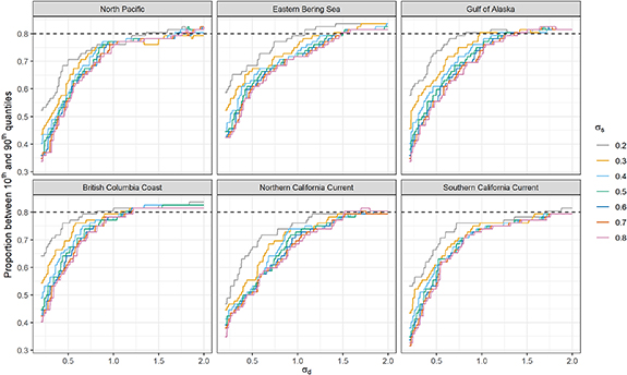
Figure A1. Results of perfect model setup: proportion of 'true' values falling between 10th and 90th quantiles of weighted prediction for different values of the shape parameters σD and σS . The dashed horizontal line indicates the target proportion.
Download figure:
Standard image High-resolution image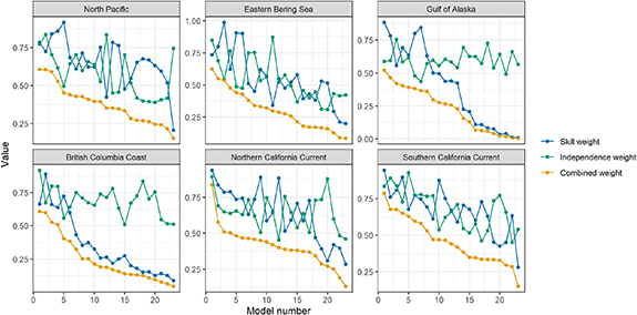
Figure A2. Skill weight, independence weight, and combined weight for 23 CMIP6 models in the six study regions. Models are sorted independently by combined weight in each region.
Download figure:
Standard image High-resolution image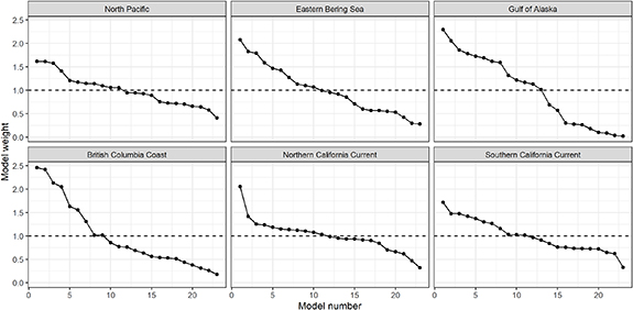
Figure A3. Combined model weights, scaled by the mean weight for each region, such that a weight of 1 (dashed horizontal line) is equal to the unweighted case. Models are sorted independently by weight for each region.
Download figure:
Standard image High-resolution image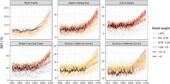
Figure A4. Observed SST (black lines) plotted against historical / SSP5-8.5 runs for 23 CMIP6 models. Normalized combined model weight for each model in each region is indicated by line color.
Download figure:
Standard image High-resolution imageWe used a separate round of model weighting for estimating the timing of different North Pacific warming thresholds under SSP2-4.5 and SSP5-8.5 (figure 5(B) in the Main Text). In this instance we only weighted models by the trend in anomalies during 1973–2022 (root mean square error for linear regression of observed anomalies on modeled anomalies). This single weighting variable reflected the goal of this part of the analysis, which was to project North Pacific warming. We used the same perfect model approach for this round of weighting, with the 'true' climatology for two periods (2001–2015 and 2031–2045) as the targets for prediction. Following the results from the previous perfect model approach, we only considered a value of σS = 0.4, and the resulting plot indicated selection of a value of σD = 0.82 (figure A5). Weights calculated with these two values of the shape parameters resulted in a greater influence of independence skill than was observed in the model weights that were used throughout the rest of the study (figure A6).

Figure A5. Results of perfect model setup for selecting the shape parameters σD for weighting CMIP6 models to hindcast and project North Pacific warming rate (figure 5(B) in Main Text). Plotted line indicates the proportion of 'true' values falling between 10th and 90th quantiles of weighted prediction for different values of σD with σS = 0.4. The dashed horizontal line indicates the target proportion.
Download figure:
Standard image High-resolution image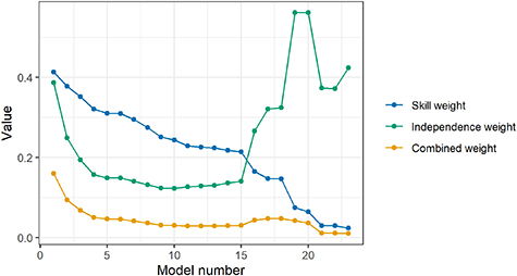
Figure A6. Skill weight, independence weight, and combined weight for weighting of North Pacific warming hindcasts and projections.
Download figure:
Standard image High-resolution image
1.3. Sockeye salmon catch analysis
Historical commercial harvests of sockeye salmon were obtained for the Chignik, Kodiak, Cook Inlet, Prince William Sound, and Southeast Alaska Management Areas from the Alaska Department of Fish and Game [32]. The South Alaska Peninsula was excluded from analysis because the majority of sockeye salmon harvests from that Management Area are for fish returning to Bering Sea natal streams.
Sockeye salmon spend varying number of years in the oceans (typically 1–5), which results in catches in a single year being comprised of fish that entered the ocean across multiple years. To calculate a single SST value for each catch year, we used a weighted average of SST values across the range of ocean entry years comprising the catch year, where the weights were the mean proportion of sockeye entering the ocean in a particular year. The sockeye salmon ocean entry proportions were calculated from age-structured adult return data (48 years, return years 1967–2014) for 15 Gulf of Alaska stocks [64]. For continuous regressions of catch on SST and FAR (figures 6(A) and (B) in the main text), we included year as a covariate in the model to account for serial dependence in the data. For the categorical model of the response of catch to high FAR values (figure 6(C) in the main text), we used weakly informative priors for all model parameters [65]. These included a Student-t distribution (3 degrees of freedom, mean = 0, SD = 3) for the intercept, slope, smooth standard deviation and error standard deviation, and a normal distribution (mean = 0, SD = 0.5) for the autocorrelation parameter.