

Abstract
Wetland soils are a key global sink for organic carbon (C) and a focal point for C management and accounting efforts. The ongoing push for wetland restoration presents an opportunity for climate mitigation, but C storage expectations are poorly defined due to a lack of reference information and an incomplete understanding of what drives natural variability among wetlands. We sought to address these shortcomings by (1) quantifying the range of variability in wetland soil organic C (SOC) stocks on a depressional landscape (Delmarva Peninsula, USA) and (2) investigating the role of hydrology and relative topography in explaining variability among wetlands. We found a high degree of variability within individual wetlands and among wetlands with similar vegetation and hydrogeomorphic characteristics. This suggests that uncertainty should be presented explicitly when inferring ecosystem processes from wetland types or land cover classes. Differences in hydrologic regimes, particularly the rate of water level recession, explained some of the variability among wetlands, but relationships between SOC stocks and some hydrologic metrics were eclipsed by factors associated with separate study sites. Relative topography accounted for a similar portion of SOC stock variability as hydrology, indicating that it could be an effective substitute in large-scale analyses. As wetlands worldwide are restored and focus increases on quantifying C benefits, the importance of appropriately defining and assessing reference systems is paramount. Our results highlight the current uncertainty in this process, but suggest that incorporating landscape heterogeneity and drivers of natural variability into reference information may improve how wetland restoration is implemented and evaluated.
Export citation and abstract BibTeX RIS
1. Introduction
Carbon (C) storage is an important process in wetlands and is cited as a goal for conservation and restoration efforts worldwide [1–3]. Wetlands contain an estimated 20%–30% of global soil organic C (SOC) [4], which varies among wetland ecosystems according to factors such as plant communities and soil properties [5–7]. Long recognized for its climate cooling effect, the wetland SOC sink has gained recent attention for its potential to mitigate human-induced climate change [8, 9]. While conserving pristine wetlands is of immediate concern for protecting global SOC stocks [8, 10], much of the existing wetland acreage has been degraded by human activities [11], and restoration remains integral to climate mitigation strategies [9]. Therefore, there is interest in refining expectations of SOC storage capacity in restored wetlands and ensuring that current practices allow targets to be met [2, 10].
The extent to which degraded wetlands can regain SOC stocks through restoration is unclear. Few restored wetlands approach SOC levels comparable to least-disturbed wetlands (hereafter, 'natural' wetlands), even after decades of recovery [12, 13]. Soil properties inherently develop slowly, but evidence of plateauing SOC accumulation well below natural levels has raised concern that restored wetlands may not reach these targets [14, 15]. Hence, there is a need to better understand how SOC stocks in restored wetlands vary compared to natural wetlands [16, 17].
In a restoration context, reference wetlands set the foundation for siting, designing, and evaluating projects for their SOC benefits. Since pre-disturbance conditions are rarely documented, information to guide restoration must come from nearby wetlands of the same type that are relatively undisturbed [18]. If restoration aims to increase SOC storage, then interventions should reflect an ecological understanding of how SOC accumulates and persists in reference wetlands [19]. Further, baseline data on SOC in reference wetlands is essential to set realistic targets and perform C accounting [20, 21]. This has become urgent given governmental efforts to create standardized natural capital accounting systems, including those for C storage (e.g. most recently for the US [22]).
Despite the critical role of reference systems, their use in wetland restoration is complicated by natural variability among individual wetlands [23]. Wetlands that appear similar can vary widely in hydrological, ecological, and biogeochemical attributes [24, 25], which makes it difficult to select references and introduces uncertainty when evaluating restored systems [26]. Classification systems are used to group wetlands, but high variability is routinely observed within classes [18, 23], meaning these systems alone may be ineffective at describing natural variability [27]. Some researchers have thus argued that the reference condition is best represented by a collection of natural systems [28, 29], or as explicitly dependent on environmental drivers [30].
A better understanding of the hydrologic drivers of wetland SOC may help constrain natural variability and provide valuable ecological information for restoration. Hydrology is considered a 'master variable' in wetland processes [31, 32], and can influence SOC through multiple mechanisms. For example, patterns of saturation and inundation control plant abundance, community composition, and primary production [33–35]. Anoxic conditions during prolonged saturation and inundation suppress microbial enzyme activity and slow decomposition, promoting the accumulation of plant-derived C in wetland soils [36, 37]. In practice, however, the relationship between wetland hydrology and SOC is less clear [7]. Hydrologic regime can differ between otherwise similar wetlands [25, 38, 39], but research is inconsistent as to how this corresponds to variability in SOC (see e.g. [7, 40]). Since no single parameter can fully describe complex wetland hydrologic regimes, improving restoration requires knowing which measurable aspects (e.g. average water level, inundation duration) are associated with SOC [41, 42].
Characterizing the role of relative topography in wetland hydrology and ecosystem processes is key to increasing the practical benefits of reference information. Relative topography can indirectly control wetland SOC through its effects on surface and groundwater flows, which in turn determine wetland hydrologic regimes [43, 44]. In restoration, this is reflected in interventions (e.g. plugging ditches, re-grading) that shape the physical landscape to achieve reference hydrologic conditions [45, 46]. Terrain analysis is increasingly recognized as an essential tool in wetland management due to its scalability and the accessibility of high-resolution elevation data [47–49].
On low-lying landscapes, natural or anthropogenic variation in topographic relief can create hydrologic conditions that support wetlands with extensive herbaceous vegetation. In addition to vegetation cover, these 'emergent' wetlands can differ from nearby forested wetlands in basin morphology, hydrology, and likely other factors that may influence SOC [50, 51]. Regardless of their historical vegetation type, wetlands are most often restored as emergent systems to promote biodiversity and wildlife habitat [52]. Certainly, quantifying the links between relative topography, hydrology, and SOC storage will help simplify reference wetland selection and inform restoration initiatives [53–55].
We measured SOC stocks in wetlands on a depressional landscape and assessed whether hydrology and relative topography explained differences among least-disturbed reference wetlands. We first compared SOC variability between representative natural and restored wetlands. We then quantified SOC stocks in a broader number of natural wetlands to determine the baseline variability on the landscape. Lastly, we tried to explain this baseline variability by examining relationships between natural wetland SOC stocks, hydrologic metrics, and terrain metrics. Our results provide insight into the collection and interpretation of reference information towards improving wetland restoration practices and evaluation.
2. Methods
2.1. Study system
Our study took place on the Delmarva Peninsula (Maryland, USA) within the mid-Atlantic Coastal Plain province (figure 1(a)). The Peninsula contains thousands of freshwater depressional wetlands ('Delmarva bays' [56]), which exist naturally as either forested or emergent (vegetated) systems. Forested bays are small (∼1 ha) closed-canopy pools with little to no herbaceous vegetation, while emergent wetlands are larger with diverse meadow-like vegetation in distinct zonal communities [51, 57]. Soils come from sandy or silty parent materials and are dominated by mineral components, although organic soils (i.e. histosols) develop in some natural bays [58]. Delmarva bays interact with shallow groundwater, and annual hydrologic patterns are characterized by seasonal (winter–spring) flooding followed by evapotranspiration-driven drawdown in the summer and fall [59]. Owing primarily to agriculture, more than two thirds of Delmarva bays have been at least partially destroyed, and those remaining have likely been hydrologically altered [56]. Recently, however, the Peninsula has seen net wetland gain [60], due in part to large-scale restoration efforts (e.g. the US Department of Agriculture's Conservation Reserve Program) [61]. Common techniques used to hydrologically restore Delmarva bays include ditch plugging, soil surface excavation, and installation of water control structures [45, 61].
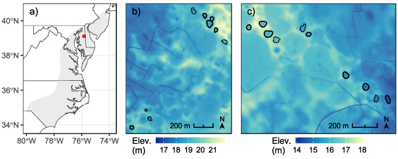
Figure 1. Location of study area (red marker) within the mid-Atlantic Coastal Plain of Maryland, USA (a). Terrain maps of the two forested wetland study sites, 'BC' ((b); 39.06° N, 75.83° W) and 'JL' ((c); 39.06° N, 75.75° W), which are ∼7 km apart. Elevation in (b) and (c) is from a digital elevation model and shown as m above sea level. Natural forested wetlands sampled for SOC stocks (n = 19) are outlined, with solid outlines indicating the 12 wetlands in which water level was monitored (emergent wetlands not shown).
Download figure:
Standard image High-resolution image2.2. Wetland SOC stocks
Our study includes data from two sampling sets to capture the range of variability in Delmarva bays. We initially chose three restored and three nearby least-disturbed ('natural') wetlands to assess spatial variability in SOC. In this set, hereafter called the 'emergent wetlands', we sampled from three vegetation zones: woody, herbaceous, and open water. After finding high variability in natural wetland SOC, we sampled an additional 19 natural wetlands (hereafter 'forested wetlands') at two sites with similar vegetation, edaphic and topographic conditions ('BC' and 'JL'; figure 1). Although emergent wetlands result from most wetland restoration/creation projects, forested wetlands are more common in the study region [52, 62] and were our focus for further baseline data.
In forested wetlands, duplicate soil cores (⩾1 m depth) were taken from the basin center and separated into five depth intervals (0–10, 10–30, 30–50, 50–75, and 75–100 cm) for analysis. To determine SOC, we first measured organic matter content in all samples by mass loss on ignition (LOI) for 16 h at 400 °C [63]. We then chose a 90 sample subset spanning the range of LOI values to measure C content using dry combustion (CHN analyzer, LECO Corp, St. Joseph, MI). We fit a linear regression between LOI and C content in the sample subset and used the fit equation (R2 = 0.99) to estimate C content from LOI in all samples. Bulk density was determined using the core method [64], with linear correction for compaction [65].
Stocks were calculated by multiplying C content, bulk density, and sample length. For each core, SOC stocks were summed over all depth increments to 1 m, and wetland values were taken as the average of duplicate cores. The mean difference between duplicates was 3.6 kg C m−2 (11.6% relative difference).
Because our initial objective was to examine soil spatial variability, our sampling approach differed in emergent wetlands. For each wetland and vegetation zone, we selected one random location and took three soil cores spaced 10 m apart (total n = 9 cores per wetland). Cores were taken to a minimum depth of 50 cm (mean = 67 cm) and separated by naturally-occurring horizons. Organic matter was determined by LOI, and C content was estimated using the linear regression fit with forested wetland samples. To compare with forested wetlands, we used a data harmonization approach: SOC density was modeled as a function of LOI using forested wetland data (sensu [66, 67]), and 1 m stocks were estimated by integrating depth functions fit with horizon values [68]. Details of soil data harmonization are in supplementary methods.
2.3. Water level data and hydrologic metrics
Continuous water level data was collected from 2018 to 2019 in a subset of study wetlands. Shallow wells were established in 12 forested wetlands and instrumented with pressure transducers (HOBO water level loggers; Onset Computer Corporation, Bourne, MA). Water levels were aggregated to daily averages for each wetland. Where necessary, data gaps were filled using nearby wells not included in this study.
We chose six metrics to capture different aspects of the hydrologic regime with potential importance in C cycling [70]. From 2019, which had average rainfall (1114 mm; figure 4(a)), we calculated: median, maximum, interquartile range, inundation duration (i.e. hydroperiod), and exposure date (i.e. the first day water level dropped below the surface). From 2018, which was wetter than average (1555 mm) but did not require gap filling, we calculated recession rate as the median daily water level decline during the growing season (May–October). We included only days when water levels declined in all wetlands and excluded days following rainstorms. A summary of metrics can be found in table 1(a).
Table 1. Metrics assessed as explanatory variables of forested wetland SOC stocks. Hydrologic metrics (a) were selected to represent distinct and fundamental aspects of wetland hydrologic regimes. Terrain metrics (b) were selected based on hypothesized or empirical relationships with hydrologic regimes as reported in literature.
| Metric | Definition/description | Mean value (min, max) |
|---|---|---|
| (a) Hydrologic (n = 12 wetlands) | ||
| Duration | Total number of days inundated (i.e. water level > 0) | 263 (228, 293) |
| Exposure | Earliest day of year exposed (i.e. water level < 0) | 222 (184, 257) |
| IQR | Interquartile range; robust index of daily water level variability (m) | 0.77 (0.49, 1.16) |
| Max | Maximum daily water level (m) | 0.76 (0.50, 1.11) |
| Median | Median daily water level (m) | 0.43 (0.18, 0.66) |
| Recession | Median daily water level decline during rain-free periods in May–Oct (cm d−1) | −1.42 (−1.85, −0.86) |
| (b) Terrain (n = 19 wetlands) | ||
| Area | Total area of wetland basin (m2) | 930 (144, 2240) |
| Catchment | Total area (wetland + upland) draining internally to wetland basin, given as relative to wetland area | 7.78 (2.93, 29.8) |
| Depth | Maximum depth of wetland basin (m) | 0.6 (0.21, 1.10) |
| Profile | Index of wetland 3D shape from conical (low) to cylindrical (high) [69] | 1.98 (0.80, 3.95) |
| RTP | Relative topographic position; mean value of deviation from mean elevation within a 500 × 500 m window | −0.87 (−1.46, −0.48) |
| Shape | Size-invariant area-to-perimeter ratio; represents complexity of 2D shape, where 1 is a perfect circle | 1.11 (1.02, 1.27) |
2.4. Geospatial data and terrain metrics
We analyzed wetland relative topography using a 1 m lidar-derived digital elevation model (DEM) of the study area [71]. Wetland basins were delineated with a Stochastic Depression Analysis tool [72], which has been used to map wetlands in the region [73]. Using the delineated wetlands and DEM, we calculated six terrain metrics (table 1(b)) associated with wetland presence [44]. These included standard descriptors (depth, area, and shape index) as well as other metrics that, based on literature reports, may contain unique information about wetland hydrology (relative topographic position, relative catchment area, and basin profile coefficient as indicators of landscape position; potential runoff inputs; wetland bathymetry; table 1(b)). Due to an extreme value, relative catchment area was transformed by  for analysis. Geospatial data was processed and analyzed in QGIS [74] using tools from Whitebox [72] and SAGA [75], and in R [v4.2.0; 76] using the sf [77] and terra [78] packages. An extended description of geocomputation is in supplementary methods.
2.5. Statistical analysis
Relationships between forested wetland SOC stocks and hydrologic/terrain metrics were quantified using multiple linear regression. Our analysis focused on two models: one with hydrologic metrics ('hydrology model'; n = 12 wetlands) and one with terrain metrics ('terrain model'; n = 19 wetlands). We included a site term in each model to account for unknown differences between our sampling sites. All statistical analysis was done in R using the car [79] and rdacca.hp [80] packages.
We expected multicollinearity, so we examined pairwise correlations and variance inflation factors (VIFs) to select minimum subsets of hydrologic/terrain metrics that characterized differences among wetlands [81]. Since our analysis was exploratory, we did not do further variable selection [80, 82], and we present regression coefficients descriptively while recognizing their uncertainty due to small sample sizes [83, 84]. Fitted models were validated by visually inspecting residuals (figures S1 and S2).
The relative importance of metrics in regression models was evaluated using variance partitioning methods [85]. Specifically, we determined the average contribution of each metric to the total variance explained in the model over all subsets of explanatory variables (i.e. hierarchical partitioning [86]). Results are expressed as partial R2 values for each metric, which sum to the multiple R2 of the model, and as % R2, which is the partial R2 divided by the multiple R2.
Commonality analysis was used to compare the variability in SOC stocks explained by hydrologic metrics, terrain metrics, and site differences [87]. First, we re-fit both models without site and chose the three metrics with the highest partial R2 in each. We then fit a third model including the selected groups of hydrologic and terrain metrics, and site (n = 12 wetlands), and partitioned variance using commonality analysis. This technique quantified each group's unique contribution to the model as well as the contributions shared among groups [87]. As in hierarchical partitioning, contributions are expressed as proportions of the model's R2. Pairwise relationships among all metrics were assessed with Pearson correlation coefficients.
3. Results
3.1. Natural variability in wetland SOC stocks
In forested wetlands, SOC stocks ranged from 19.7 to 51.0 kg m−2 (mean = 32.2 kg m−2 SD = 8.40, CV = 26.1%; figure 2). Natural emergent wetland estimates spanned a similar range (14.0–49.4 kg m−2), and two of the three wetlands contained soils dominated by organic materials. Restored emergent wetlands had a narrower range of estimated SOC stocks (10.9–28.1 kg m−2), although several point estimates fell within the ranges of both types of natural wetlands (figure 2).
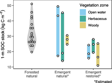
Figure 2. Variability in SOC stocks among forested natural wetlands, alongside point estimates from vegetation zones in natural and restored emergent wetlands. Shaded areas show range of values.
Download figure:
Standard image High-resolution imageThere was high spatial variability in emergent wetland SOC. Mean estimated stocks were highest in open water (36.7 kg m−2) for natural wetlands and in herbaceous vegetation (24.1 kg m−2) for restored wetlands (figure 2). Natural wetlands had higher among-zone variability (i.e. mean of CVs for each wetland; 36.3%) and among-wetland variability (i.e. mean of CVs for each zone; 40.5%) compared to restored wetlands (among-zone CV = 18.9%, among-wetland CV = 27.3%). Variability among natural wetlands was driven more by open water (CV = 46.7%) and herbaceous (CV = 64.4%) than by woody vegetation (CV = 10.6%; figure 2). For the herbaceous zone, all restored SOC stock estimates fell within the natural range.
3.2. Wetland SOC stocks as a function of hydrologic metrics
As expected, there was multicollinearity and strong correlations among hydrologic metrics (figure 3). Since water levels in all wetlands followed a similar seasonal pattern (figure 4(b)), we assumed correlated metrics reflected the same hydrologic dynamics, and proceeded with a subset containing duration, max, and recession. The strongest correlation in this subset was between duration and max (r = 0.44).

Figure 3. Pearson correlation matrix of hydrologic metrics (duration, exposure, IQR, max, median, recession) and terrain metrics (area, catchment, depth, profile, RTP, shape) in natural forested wetlands. Outlined box contains correlations between a hydrologic and a terrain metric. Correlations between two terrain metrics represent data from 19 wetlands; all other correlations represent a 12 wetland subset for which hydrologic data was available. Note that catchment was transformed by  .
.
Download figure:
Standard image High-resolution image
Figure 4. Daily 2019 (a) mean temperature and total precipitation, and (b) water level in a subset of forested wetlands. Water levels shown as daily means of wetlands at study sites 'JL' and 'BC' (n = 7 and 5) and for each wetland separately (grey lines). Some wetland water levels appear to flatten as wells dried and transducers read constant values. Climate data was collected at JL weather station.
Download figure:
Standard image High-resolution imageThe hydrology model explained variability in SOC stocks (R2 = 0.75, R2 adj.= 0.61), but individual metrics differed in their contributions (table 2). Recession was the most important, with a higher contribution (37.7%) than the other two combined (20.8%), while duration was relatively unimportant. Both recession and max were positively associated with SOC stocks (β = 0.52 ± 0.24 and 0.53 ± 0.23, respectively); in other words, wetlands with deeper water and slower drying rates tended to have higher SOC stocks. The negligible r2 value of max, however, shows its contribution to the model (% R2 = 13.4) was likely due to suppression of residuals rather than by direct association with SOC stocks. Recession was the only metric that explained variability in SOC stocks individually (r2 = 0.34).
Table 2. Results of multiple linear regression of SOC stocks as a function of hydrologic metrics in natural forested wetlands (n = 12).
| Metric | r2 | VIF | β | P | Partial R2 | % R2 |
|---|---|---|---|---|---|---|
| Site (JL) | 0.28 | 2.9 | −1.62 ± 0.62 | 0.04 | 0.31 | 41.6 |
| Recession | 0.34 | 1.6 | 0.52 ± 0.24 | 0.07 | 0.28 | 37.7 |
| Max | <0.01 | 1.6 | 0.53 ± 0.23 | 0.06 | 0.10 | 13.4 |
| Duration | <0.01 | 3.1 | 0.20 ± 0.33 | 0.57 | 0.06 | 7.4 |
| Hydrology model: R2 = 0.75; R2 adj. = 0.61; P = 0.03. | ||||||
Model statistics: marginal R2, adjusted R2 (R2 adj.), P value (P).Statistics for each term: squared bivariate correlation with SOC stocks (r2), variance inflation factor (VIF), beta coefficient (β ± std. err.), P value (P), partial contribution to multiple R2, and percent contribution to multiple R2.
Site was an important component in the hydrology model (% R2 = 41.6). SOC stocks were lower in JL than in BC (β = − 1.62 ± 0.62), and this difference was not explained by hydrologic metrics. Although we did not include interaction terms in the model, pairwise relationships between hydrologic metrics and SOC stocks appeared to depend on site (figures 5(a)–(c)). Within BC, all three metrics had higher slopes and explained more variability (mean r2 = 0.69) than within JL (mean r2 = 0.14).

Figure 5. Relationships between upper 1 m SOC stocks and hydrologic/terrain metrics in natural forested wetlands (n = 19). The three hydrologic ((a)–(c)) and three terrain ((d)–(f)) metrics that contributed the most to their respective model are shown; diamond-shaped markers are wetlands without water level data (i.e. only included in terrain analysis; n = 7). Linear best-fit lines are shown separately for each study site ('BC', 'JL').
Download figure:
Standard image High-resolution image3.3. Relationships between wetland relative topography, hydrology, and SOC stocks
There were strong correlations between terrain metrics and hydrologic metrics (figures 4 and S3). The strongest correlation was between depth and max (r = 0.87), which was expected given that depth is effectively an estimate of max based on relative topography. Duration and recession were most strongly correlated with RTP and profile, respectively (r = −0.70 and 0.66). Among terrain metrics, catchment and depth were correlated (r = −0.79) so we excluded the former from further analysis.
As with hydrology, individual metrics contributed unevenly to the terrain model (table 3). Profile was the most important (% R2 = 58.0) and was positively associated with SOC stocks (β = 0.74 ± 0.34); that is, wetlands that were more cylindrical (i.e. had flatter bottoms) tended to have higher SOC stocks (figure 5(d)). Despite correlating with hydrologic metrics, depth and RTP had minor contributions to the terrain model (% R2 = 12.5 and 9.5). Site was a minor component (% R2 = 7.6) and relationships between terrain metrics and SOC stocks did not appear to consistently differ between sites (figures 5(d)–(f) and S4).
Table 3. Results of multiple linear regression of SOC stocks as a function of terrain metrics in natural forested wetlands (n = 19).
| Metric | r2 | VIF | β | P | Partial R2 | % R2 |
|---|---|---|---|---|---|---|
| Profile | 0.41 | 3.0 | 0.74 ± 0.34 | 0.05 | 0.31 | 58.0 |
| Depth | 0.07 | 2.7 | −0.30 ± 0.32 | 0.38 | 0.07 | 12.5 |
| RTP | 0.10 | 1.7 | −0.02 ± 0.26 | 0.94 | 0.05 | 9.5 |
| Shape | 0.06 | 2.3 | 0.06 ± 0.30 | 0.85 | 0.05 | 8.5 |
| Site (JL) | 0.07 | 2.4 | −0.03 ± 0.59 | 0.96 | 0.04 | 7.6 |
| Area | 0.02 | 1.9 | −0.08 ± 0.27 | 0.77 | 0.02 | 3.9 |
| Terrain model: R2 = 0.54; R2 adj. = 0.30; P = 0.10. | ||||||
Model statistics: multiple R2, adjusted R2 (R2 adj.), P value (P).Statistics for each term: squared bivariate correlation with SOC stocks (r2), variance inflation factor (VIF), beta coefficient (β ± std. err.), P value (P), partial contribution to multiple R2, and percent contribution to multiple R2.
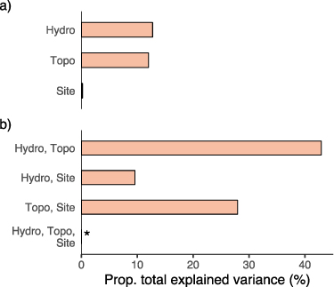
Commonality analysis revealed that hydrologic and terrain metrics both explained a common portion of variability in wetland SOC stocks (figure 6). Hydrologic metrics were represented by duration, max, and recession, and terrain metrics by depth, profile, and shape. The largest component was that shared by the hydrologic and terrain groups, which contributed 42.9% of the model's R2 value. Both groups had similar unique components (hydrologic = 12.8%, terrain = 12.0%). The unique component of site was approximately zero (0.2%); nearly all its contribution was shared by terrain or (to a lesser extent) hydrologic metrics. Variability shared among all groups was a small negative value (−5.4%), which was likely due to sampling error and can be considered zero [88].
Figure 6. Variance partitioning of wetland SOC stocks. Colored bars are proportions of explained variance (a) attributed uniquely to hydrologic metrics ('Hydro'), terrain metrics ('Topo'), and unknown sampling site differences, and (b) shared among those groups. Hydrologic metrics included recession rate, maximum water level, and inundation duration; terrain metrics included basin profile coefficient, depth, and shape index. The asterisk in (b) denotes a component with a negative contribution (−5.4%) shown as zero. The total variability explained by the model (i.e. multiple R2) was 0.85 (R2 adj. = 0.60).
Download figure:
Standard image High-resolution image
4. Discussion
Focusing on one of the most common types of wetlands worldwide—seasonal depressional wetlands—we show extensive variability in SOC storage. This was evident in both natural and restored wetlands, and to such an extent that it was difficult to distinguish wetland types based on their SOC content. This finding raises two pertinent questions: how much do SOC stocks vary among wetlands on any landscape? And can we explain SOC variability by quantifying wetland-scale differences in hydrology and relative topography? In the following, we address these questions and discuss the implications of our study for how reference conditions are determined in wetland restoration.
4.1. High natural variability in wetland SOC stocks
We measured a wide range of SOC stocks among wetlands that would be considered replicates for most purposes. Wetlands are often classified based on vegetation and hydrogeomorphology, and wetland types are widely used to approximate functions in lieu of empirical data [89]. However, despite their shared vegetation type and hydrogeomorphic class (depressional), as well as their proximity to one another, the 19 forested wetlands we sampled had SOC stocks spanning values characteristic of mineral wetlands (∼20 kg C m−2) to those of organic wetlands (>50 kg C m−2; table 4). Mean stocks in our forested wetlands were 32.2 ± 8.4 kg m−2; in comparison, a recent analysis of 529 inland wetlands, which spanned vegetation types and ecoregions throughout the conterminous US, estimated mean SOC stocks at 19.7 ± 10.6 kg m−2 [90]. We compiled a list of relevant studies encompassing a range of wetland types and found that high within-type variability is common (table 4). This suggests that caution should be broadly applied when assuming that wetland types, as defined by existing classification systems, reflect variability in ecosystem processes [27, 91–93].
Table 4. Variability in wetland SOC stocks from this study (in bold) and literature reports. Data are field-measured from natural (least-disturbed) non-tidal freshwater wetlands in temperate climates. Wetland types are as described in the studies, and soil type (O = organic, M = mineral), if indicated, is self-defined by the publication. Only studies reporting 1 m stocks are included. Ranges of values are shown if given. N = number of wetlands.
| 1 m SOC stock (kg C m−2) | ||||
|---|---|---|---|---|
| Wetland type | N | Mean ± std. dev. | Range | References |
| Coastal Plain depressional (O) | 3 | 73.3 ± 47.4 | 22.1–115.7 | Fenstermacher et al [108] |
| Seasonally inundated (O) | 6 | 68.3 ± 44.1 | Pearse et al [109] | |
| Fen | 6 | 64.5 ± 8.6 | Zhang et al [110] | |
| Floodplain forest (O) | 15 | 53.3 ± 9.7 | 38.0–68.7 | Ricker and Lockaby [111] |
| Forested depressional | 19 | 32.2 ± 8.4 | 19.7–51.0 | This study |
| Marsh | 5 | 25.2 ± 9.3 | Zhang et al [110] | |
| Forested riparian | 29 | 24.6 ± 9.6 | 11.7–49.5 | Ricker et al [112] |
| Coastal swamp oak forest | 6 | 24.1 ± 13.6 | 13.8–43.3 | Kelleway et al [113] |
| Coastal Plain depressional (M) | 11 | 21.5 ± 17.2 | Fenstermacher et al [108] | |
| Floodplain forest (M) | 15 | 19.3 ± 10.5 | Ricker and Lockaby [111] | |
| Marshy meadow | 5 | 16.0 ± 2.3 | Zhang et al [110] | |
| Floodplain forest (M) | 10 | 14.9 ± 3.3 | 9.5–19.2 | Heger et al [114] |
| Floodplain grassland (M) | 5 | 14.4 ± 3.6 | 11.2–18.3 | Heger et al [114] |
| Grassland playa | 17 | 10.6 ± 4.1 | O'Connell et al [115] | |
We also found that SOC varied within spatially heterogeneous wetlands. Accounting for spatial variability is essential for accurately assessing wetland functions and can help to identify drivers of function in reference systems [94, 95]. In our natural emergent wetlands, estimated SOC stocks varied among vegetation zones, but in an inconsistent pattern among wetlands. Spatial variability was lower in restored emergent wetlands, which aligns with studies indicating that soil properties are more spatially homogeneous in restored wetlands [96, 97]. While vegetation communities are thought to influence wetland SOC storage [7, 98, 99], our results suggest that vegetation type may not be a reliable indicator of within-wetland SOC variability. We did not directly measure productivity, but we expect its variability to be dominated by vegetation type, as reported elsewhere (e.g. [100]). Instead, other factors (e.g. flooding patterns and soil properties that affect oxygen availability and decomposition [101]) likely contribute to spatial variability within these wetlands.
Our observations of high natural variability support a revised strategy for defining reference conditions (e.g. [102]). In small datasets like ours, high variability limits the ability to evaluate restored wetlands relative to references. Incorporating attributes like hydrology can help interpret reference information (as we address in the following section), but significantly increasing precision in reference conditions requires extensive data and a thorough understanding of landscape variability [103]. Constraints on time and funding often put these conditions out of reach for practitioners. With outcomes unpredictable, restoration assessment would benefit from a more rigorous treatment of uncertainty and a greater focus on the natural range of variability [104, 105]. For example, strategies like setting targets for groups of wetlands (rather than for individual wetlands) and reducing the precision of targets acknowledge ecosystem dynamism and promote heterogeneity [106, 107]. Importantly, our results also suggest that estimates of restored wetland 'C storage potential' should be accompanied by uncertainty analysis based on landscape-scale variability.
4.2. Complex role of hydrology in explaining SOC stock variability among wetlands
Water level recession rate had the strongest relationship with SOC stocks, while standard hydrologic descriptors, notably inundation duration (i.e. hydroperiod), explained relatively little variability among wetlands. Measures of duration and average water level are commonly used in wetland restoration to set performance standards and evaluate success [116, 117]. Although these metrics have been linked to wetland processes [118, 119], our results indicate that the most relevant aspects of the hydrologic regime may depend on the system and process of interest [54].
The importance of recession rate suggests a key role of drying processes in wetland SOC storage. Recession rate represents wetland response to negative water fluxes, mainly evapotranspiration and groundwater outflow [38]. Human management at the catchment scale has been shown to affect wetland recession rates by altering upland forest evapotranspiration [120]. Wetlands that dry faster may have soils with increased oxygen diffusion, increased temperature sensitivity of respiration, and more frequent wet–dry cycles; all of which can promote C loss through mineralization [121–123]. Recent reports have linked recession rates to other ecological and biogeochemical variables [124–126], which implies a broader importance in wetland function that should be examined in future studies.
Interestingly, site-scale differences appeared to modulate hydrology–SOC relationships. Such differences could include, for example, proximity to drainage ditches, absolute elevation, forest age, and adjacent land use [120, 127, 128]. While studies have established that large-scale factors like climate and geological setting can be important controls of SOC (e.g. [129]), these did not vary within our study area. Furthermore, since our forested wetlands lacked emergent vegetation and most had the same soil type (i.e. map unit; table S2), we assumed in situ production and soil properties were relatively uniform, but fine-scale spatial variability in these factors could affect SOC storage [40, 118, 130, 131]. For example, soil texture can vary among neighboring wetlands [132, 133], including those within the same soil map unit [134], and we did note that deeper layers at BC had finer textures than at JL (data not shown). Studies have shown that soil physical properties may interact with water level to influence wetland C processes [135, 136], so it is plausible that soil texture contributed to the site differences we observed. Similarly, though in situ production was likely a minor source of variability, terrestrial inputs are also important sources of C, and may have interactive effects with hydrology on wetland C budgets [137–139]. Regardless of its cause, spatial variability in wetland hydrology–SOC relationships may occur within limited areas and should be considered when setting expectations for restored wetlands.
Our study joins a growing list that have found complex or unclear relationships between wetland hydrology and SOC (e.g. [6, 7, 109, 140]). In addition to other sources of variability, these results suggest that hydrology is a multifaceted and indirect driver of wetland SOC [141, 142]. Hydrology influences wetland C processes through numerous mechanisms such as dissolved organic matter flows, temperature, and, predominantly, soil oxygen diffusion [139, 141, 143]. Despite the negative effect of water level on oxygen content (and thus decomposition [143]), persistent water saturation can maintain anoxia long after inundation recedes [144]. Further, inundation does not always slow decomposition [142]. Decomposition rates also depend on factors such as organic matter chemistry, physicochemical stabilization, microbial communities, and the availability of alternative electron acceptors [145–147]. Overall, though hydrology is a 'master variable' in wetland function, its breadth of biogeochemical influence makes it difficult to quantify its role in specific processes.
4.3. Relative topography and hydrology provide similar information about wetland SOC stocks
We found that hydrology and relative topography explained much of the same variability in wetland SOC stocks. Relative topography provides the physical basis for wetland hydrology [43, 148], and therefore may help characterize wetland ecosystem processes that respond to the hydrologic regime [149]. Accordingly, our results support evidence that cylindrical (i.e. flat-bottomed) wetlands have slower recession rates [150–152] and indicate that these wetlands may also have higher SOC stocks. Relative topography can also reflect other forms of landscape-scale variability [38, 153]; for example, the basin-forming processes that determine wetland bathymetry may also affect sedimentation and soil texture [69, 154]. Developing a mechanistic understanding of the relationships between relative topography, hydrology, and wetland processes is imperative to inform how restoration interventions can support functions like SOC storage.
Hydrology did not offer a clear advantage over relative topography in explaining SOC stock variability among our wetlands. This finding is significant in that relative topography is a far more practical tool for large-scale analyses. Terrain metrics can be rapidly computed over large areas with publicly-available remote sensing data, in contrast to water level data, which is more expensive and time-consuming to obtain [49]. It should be noted that human-made structures (e.g. ditches, tile drainage) that modify wetland hydrology may not be detected by remotely-sensed terrain metrics [128]; thus, care should be taken when scaling to broader areas.
Relative topography may even be a preferable indicator when only short-term hydrologic data is available. Although 2019 represented average water conditions, wetland hydrologic tendencies can shift over time with changes in catchment land cover, regional water withdrawals, and climate-driven precipitation patterns [119, 155, 156]. Hydrologic non-stationarity is especially likely in heavily altered areas, where contemporary conditions may uncouple from 'slow' variables like SOC that develop over decades to centuries [157, 158]. Relative topography is less responsive to nonlocal disturbance and could therefore more robustly represent reference wetland conditions at these time scales.
5. Conclusion
Understanding natural variability in ecosystem processes is critical for successful restoration. In wetlands, variability in C cycling is widely recognized, but attention has mainly centered on C fluxes [159]. We found that SOC stocks varied substantially among neighboring least-disturbed wetlands with similar vegetation and hydrogeomorphology. In a restoration context, this implies that reference conditions have inherent uncertainty, and that success should be evaluated against the range of natural variability [105]. Although hydrologic metrics explained some variability in SOC stocks, our results highlight the complex and context-dependent relationships between wetland hydrology and ecosystem processes. We therefore caution that a reliance on hydrology as the primary predictor of wetland processes risks undervaluing the role of other potential drivers. Lastly, wetland terrain metrics were correlated with hydrologic metrics and explained similar variability in SOC stocks. This result is promising given that the physical landscape can be analyzed at large scales and offers an interface for management to affect wetland processes [53]. As focus grows on quantifying C benefits in restoration, the importance of appropriately defining reference conditions is paramount. In the foreseeable future, determining how much SOC a wetland 'should have' is likely to remain unfeasible, but C accounting practices can still have robust ecological foundations by integrating natural variability and its drivers into reference frameworks.
Acknowledgments
We gratefully acknowledge The Nature Conservancy for allowing us access to the study sites and for their stewardship of the land. We thank Dr C Nathan Jones for maintaining wetland wells and water level data, Drs Alec Armstrong, Kelly Hondula, and Christine Maietta for their advice throughout the research process, and Jenny Lees, Bianca Noveno, and Maggie Tan for their indispensable field and lab assistance. Financial support was provided for authors by NSF DBI-1639145 and for research by NSF DEB-1856200.
Data availability statement
The data that support the findings of this study are openly available at the following URL/DOI: https://doi.org/10.5281/zenodo.7791606 [160].
Supplementary material (0.2 MB PDF)