

Abstract
Photovoltaic power (PV) is the fastest-growing source of renewable electricity. Making reliable scenarios of PV deployment requires information on what drives the spatial distribution of PV facilities. Here we empirically derive the determinants of the distribution of utility-scale PV facilities across six continents, using a mixed effects logistic regression modelling approach relating the occurrence of over 10 000 PV facilities to a set of potential determinants as well as accounting for country and spatially correlated random effects. Our regression models explain the distribution of PV facilities with high accuracy, with travel times to settlements and irradiation as the main determinants. In contrast, our results suggest that land cover types are not strong determinants of the PV distribution, except for Asia and Africa where the PV distribution is related to the presence of agriculture, short natural vegetation and bare land. For Europe and Asia a considerable part of the variance in PV distribution is explained by inter-country differences in factors not included in our fixed determinants. Relevant determinants identified in our study are in line with the main assumptions made in cost of electricity (COE) maps used in the IMAGE integrated assessment model (IAM). However, we found correlations (Spearman ρ) of −0.18–0.54 between our PV probability maps and IMAGE's COE maps. These may partly be explained by conceptual differences between our empirically-derived probability maps and the COE maps, but we also recommend using higher-resolution maps of PV potential and COE computations such as used in IAMs.
Export citation and abstract BibTeX RIS

Original content from this work may be used under the terms of the Creative Commons Attribution 4.0 license. Any further distribution of this work must maintain attribution to the author(s) and the title of the work, journal citation and DOI.
1. Introduction
Renewable electricity sources are expected to play a vital role in the transition towards a net-zero emission energy system. Photovoltaic (PV) systems are the fastest-growing source with the steepest cost reductions of renewable electricity (IEA 2021, REN21 2021). Capacity additions of more than 100 gigawatts per year are expected in the next decade (Creutzig et al 2017, IEA 2020). Reliable scenarios of PV electricity supply require knowledge on the spatial distribution of PV facilities and the underlying determinants. Besides available solar radiation, studies have identified a range of factors that determine a location's suitability for a PV facility, including biophysical factors (e.g. land cover, slope), infrastructure (e.g. distance to roads, urban settlements and transmission lines), ecological factors (e.g. protected areas), and economic factors (investments and other costs) (e.g. Hernandez et al 2015, Köberle et al 2015, Al Garni and Awasthi 2017, Aly et al 2017, Agyekum et al 2021).
Studies of regional or global PV potential often use a-priori suitability maps based on these (bio)physical and economic determinants (e.g. Köberle et al 2015, Tröndle et al 2019, Dupont et al 2020, Gernaat et al 2021, Ouchani et al 2021).
Typically, maps of physical potential are established first, based on irradiation and temperature. Then, the geographical PV potential is determined by excluding areas deemed unsuitable, such as forests or urban areas. Subsequently, the physical and geographical potential can be combined with technical and cost assumptions to calculate technical or economic PV potentials and maps for use in energy and climate scenarios (Hoogwijk 2004, Köberle et al 2015, Gernaat 2019, Oakleaf et al 2019, Dupont et al 2020). Studies on PV potential often make a-priori assumptions on the importance of the factors influencing the geographical, technical and economic potential. Empirical evidence on the actual locations of PV facilities may however differ from these a-priori maps and can thus be used to update these priors (e.g. Hernandez et al 2015).
Here, we propose an empirical approach to investigate the determinants of the global distribution of PV facilities, linking actual locations of ∼10 000 utility-scale (median capacity 12 MWp) PV facilities across the globe to physical, geographical, infrastructure and ecological determinants. By establishing continent-specific mixed effect logistic regression models, we investigate what determines the actual distribution of PV facilities across the globe. Regression model approaches have been applied to identify the determinants of the distribution of small-scale PV facilities within a country (e.g. Thormeyer et al 2020, Balta-Ozkan et al 2021), confirming that besides available solar radiation socio-demographic factors play an important role in the spatial distribution of PV facilities. A near-global study revealed that accessibility is an important determinant of probability of occurrence of PV facilities (Dunnett et al 2022). Kruitwagen et al (2021) show that PV facilities are often sited on cropland, but indicate that land cover is not the single driving factor in PV distribution. Here, we focus on identifying determinants of the global distribution of large-scale (utility-scale) PV facilities. Secondly, we create high-resolution probability maps based on our regression models and compare our results to existing a priori maps used in the integrated assessment model (IAM) IMAGE, which are among the most transparent and spatially detailed estimates (Hoogwijk 2004, Gernaat et al 2021). Our results provide insights into the global expansion of utility-scale PV facilities and are thus useful for many applications such as econometric analyses and IAMs.
2. Methods
2.1. Global distribution of utility-scale PV
The Wiki-Solar dataset is the only available inventory providing information on the location and technological characteristics of utility-scale PV facilities around the globe at the time of our study (Wiki-Solar). From this dataset, we selected the 10 306 PV facilities currently operating or near completion, for which latitude and longitude are given, and which are non-floating 4 . Capacities range from 0.9 to 9400 MWp with a median value of 12 MWp (figure 1). The global total capacity in the Wiki-Solar dataset is 318 GWp. Kruitwagen et al (2021) recently estimated 350 GWp PV global capacity larger than 1 MWp. IRENA (2021) estimated a global PV capacity of 707.5 GWp, of which 55% is utility-scale (IEA 2021), corresponding with 389 GWp.
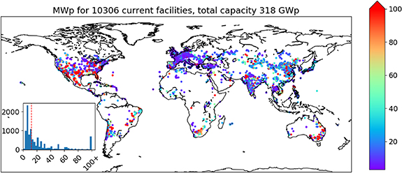
Figure 1. Distribution and capacities of the 10 306 PV facilities currently operating or near-completion available from Wiki-Solar (Wiki-Solar). The colour bar and histogram show capacity in MWp, the red line in the histogram is the median value (12 MWp).
Download figure:
Standard image High-resolution image2.2. Determinants
Based on findings reported in the literature, we identified a set of possible predictors (covariates, explanatory variables) of utility PV locations (Hernandez et al 2015, Köberle et al 2015, Al Garni and Awasthi 2017, Aly et al 2017, Agyekum et al 2021, Oakleaf et al 2019), Ouchani et al 2021, Dunnett et al 2022). See SI table S1 for an overview of the considered predictors. We refer to the predictors from now on as determinants. We obtained determinant values from various publicly accessible sources with global coverage. Table 1 includes references as well as a rationale behind including each predictor.
Table 1. Potential determinants used in the regression modelling, based on literature review detailed in SI table S1. Land cover type fractions vary between 0 and 1 and are based on aggregating the ESA CCI land cover types into agriculture, forest, short natural, urban, bare, wetland and water, see SI table S2. Resolution is given in degrees ° or arcseconds '' with the approximate equivalent distance in meters at the equator.
| Determinant (unit) | Rationale | Original resolution | Database sources |
|---|---|---|---|
| Irradiation (kWh m2 yr−1) | Higher irradiation -> higher PV yield | 0.25° (∼30 km) | ERA5, Hersbach et al (2018) |
| Elevation (m) | Higher elevation -> less accessible for construction and maintenance | 3'' (∼90 m) | MERIT, Yamazaki et al (2017) |
| Slope (degree) | Higher slope -> less suitable for construction and maintenance | — | MERIT, this study |
| Distance to roads (m) | Larger distance -> less accessible for construction and maintenance | 10'' (∼300 m) | GRIP, Meijer et al (2018), this study |
| Distance to transmission grid (km) | Further away: more cost to deliver electricity. | — | Arderne et al (2020), this study |
| Travel times to nearest settlement of >5000 inhabitants (hours) | Indicative of energy demand (proximity of settlements) | 30'' (∼1 km) | Nelson et al (2019) |
| Protected status (yes/no) | PV facilities less likely in protected areas | 10'' (∼300 m) | WDPA (UNEP-WCMC and IUCN, 2017) |
| Land cover fractions | PV facilities more likely in e.g. agriculture or grassland than forest | 10'' (∼300 m) | ESA CCI, this study |
We computed the 30 year (1988–2017) average annual irradiation from hourly incoming solar radiation from ERA5 reanalysis data, obtained through Copernicus' Climate Data Store (Hersbach et al 2018).
We derived elevation data from the MERIT Digital Elevation Model (Yamazaki et al 2017), from which we computed slope using the gdaldem function (GDAL 2020).
We determined distance to roads as the Euclidean distance to road types I–V in the GRIP dataset (Meijer et al 2018). We computed distance to the transmission grid using the gdal proximity function (GDAL) on the global MV (>10 kV) and HV (>70 kV) transmission lines from Arderne et al (2020). We then computed distance in kilometers using the v.distance function from the Geographic Resources Analysis Support System (GRASS). Travel times to the nearest settlement with a population >5000 are provided by Nelson et al (2019) 5 , representing the year 2015.
We obtained the global distribution of protected areas (such as nature reserves) from the World Database on Protected Areas (WDPA, UNEP-WCMC and IUCN 2017).
We include land cover types from the ESA CCI land cover map from 2000 as indicative of preinstallation land cover (out of 10 306 current facilities in the Wiki-Solar dataset, globally, only two facilities were built in 2000 or earlier).
We resampled or aggregated all data from their original resolution (see table 1) to a 0.011° resolution (40'', ∼1.5 km2 at the equator). This gives sufficient detail at the global scale while keeping the computational costs relatively low, and the majority of PV facilities are smaller than the grid cells at this resolution 6 . We computed land cover fractions by aggregating the land cover types at 300 m resolution to seven categories at 0.011° resolution (SI table S2).
2.3. Regression modelling
We used mixed effects logistic regression modelling, fitting a logistic curve to the binary response variable (presence or absence of a PV facility) to study how the probability of PV occurrence depends on the determinants mentioned above (as fixed effects) and country as well as spatially correlated random effects. Country names, obtained from marineboundaries.org (EEZ), are included as random determinant capturing, among others, policy effects not included in the list of determinants in table 1. Previous studies identified policy-related factors such as policy as critical for PV presence (e.g. Thormeyer et al 2020). However, in absence of a single global policy indicator and because most users of PV potential maps use policy as a separate exogenous variable, we included it here as part of the 'country' determinant. Country is included as a random effect because as a fixed effect it would take too many degrees of freedom.
We selected absences randomly from land grid cells where no PV facility is present yet, and which are not fully covered by water, permanent snow and ice. We set the number of absences to 10 times the number of presences (Barbet-Massin et al 2012). Furthermore, we weighted the selection of absences latitudinally to account for the latitudinal change in grid size. Figures S1–S6 shows the distribution of presences and absences, and figures S7–S12 and S13–S18 show the distribution of the determinants over these locations. We log-transformed road distance, grid distance, travel times, elevation and slope to reduce their positive skew.
We established a regression model for each continent, which allows us to study whether there are inter-continental differences in the determinants of PV facility distribution. We thus create regression models for North America (2272 facilities), South America (361), Europe (3432), Asia (3940), Africa (182) and Oceania (102) (see SI table S3).
Before fitting the models, we checked for multicollinearity in the determinants using variance inflation factors (VIFs) and removed determinants with a VIF > 5 (Menard 2001, Zuur et al 2009), to obtain a non-redundant predictor set (Čengić et al 2020). Based on the VIFs, we removed grid distance for Europe, and road distance for North America. We further excluded the fraction of forest land, which was correlated to the proportion of agricultural land, to avoid rank deficient fixed-effect model matrices due to the additive nature of the land cover fractions.
We built a generalised linear mixed model for each continent (see SI text 1) using the R implementation of the Integrated Nested Laplace Approximation (INLA, Rue et al 2009, Martins et al 2013) of R-INLA (Lindgren et al 2011, Lindgren and Rue 2015). INLA is a Bayesian method that utilizes the Laplace Approximation to find the optimal values for model coefficients. It takes into account spatial autocorrelation in the response variable (Mielke et al 2020), as PV facilities tend to be spatially clustered (see figures 1 and S1–S4). INLA is very efficient in the modelling of spatially correlated random effects, because it uses an underlying structure ('mesh') that consists of a limited number of locations. The spatially correlated random effects are optimized for these locations only. For data point locations that are not covered by the mesh locations, the spatial effect is calculated as an interpolation of surrounding mesh locations. This strategy greatly reduces the computational complexity compared to directly optimizing the spatially correlated random effects for all data point locations. We use the default priors given in R-INLA (see SI text 2). Before model fitting we scaled the determinant values to a mean of 0 and a standard deviation of 1, as measurement scales varied greatly among the determinants. We performed all subsets modelling, building models for all possible combinations of determinants, and selected the best-supported model based on the Widely Applicable Bayesian Information Criterion (Watanabe 2013). We calculated model performance measures area under the curve, true positive rate (sensitivity), true negative rate (specificity) and true skill statistic (TSS). We tested for residual spatial autocorrelation using Moran's I. SI text 3 provides more detail on these model performance statistics.
Finally, to quantify the relative importance of each determinant, we predicted the probability of PV occurrence using the continent-specific best-supported models and randomized values for the determinant of concern. We then correlated these predictions with the predictions of the models using the original data, and we computed the relative importance as one minus the Spearman rank correlation coefficient (Thuiller et al 2016). We also created partial dependence plots for important determinants by predicting the probability of occurrence with all determinants set to their mean value except for the determinant of interest. Finally, we used the best-supported models to create for each continent a map displaying the ranked probability of occurrence (PoO) of a PV facility.
2.4. Comparison with PV suitability map in IMAGE
Integrated assessments models (IAMs) use data on PV potential as a key input. The Integrated Model to Assess the Global Environment (IMAGE) is a prime example of such a model (e.g. Köberle et al 2015, Gernaat 2019). The key input for IMAGE are maps of economic potential (i.e. PV potential below a certain cost) at grid level, identifying potentially attractive areas based on optimisation, which are translated into regional cost-supply curves used in energy and climate scenario studies.
- (a)First, the theoretical potential is computed per grid cell, based on the available amount of solar radiation annually.
- (b)Then, the geographic potential equals the theoretical potential in areas deemed suitable for PV facility construction. Excluded areas are, for instance, protected reserves, high altitudes and forests (see table S3).
- (c)The technical potential is computed using temperature and PV panel efficiency, which determines how much the geographic potential can be transformed into electricity (usually, a fixed efficiency is set for all grid cells).
- (d)Finally, PV costs are computed based on investment, transmission and maintenance costs. A production cost, or cost of electricity (COE), map is created by dividing the costs by the technical potential. Economic potential is defined as the PV generation potential below a certain cost level, and the grid-cell-specific cost map can then be used to create country- or region-specific cost-supply curves. For more detail see SI text 4, see Gernaat (2019), Gernaat et al (2021) or Köberle et al (2015).
We compared our maps of PV facility probability with the IMAGE COE maps at their 0.5° resolution. Upfront, we expected locations with a high PV facility probability to have low PV production costs (in $/kWh). To test this, we quantified the Spearman rank correlation between 1 minus the occurrence probability and the COE. We looked at the complement of the occurrence probability (1-PoO) rather than the probability itself such that a larger positive correlation denotes a higher degree of agreement. We preferred the Spearman rank correlation over alternative correlation coefficients because we expected a monotonous but not necessarily linear relationship. For grid cells excluded from PV deployment in IMAGE, we set the COE to the maximum value within the continent +1, enabling us to include all grid cells in the analysis.
3. Results
3.1. Regression models: determinants of PV distribution
The continent-specific best-supported models explain the distribution of PV facilities well, as exemplified by high values for model performance measures (see table 2). When excluding country names, the model performance drops significantly for Europe and Asia (see SI table S6). This indicates that inter-country differences in factors not included in our fixed determinants play an important role in PV distribution. In North and South America, Africa and Oceania the country random effect plays little to no role.
Table 2. Model performance based on AUC: area under the curve, TPR: sensitivity (true positive rate), TNR: specificity (true negative rate), TSS: true skill statistic, Moran's I: a measure of residual spatial autocorrelation. Please see SI text 3 for more details on these model performance measures. SI table S6 shows the model performance without country included.
| North America | South America | Europe | Asia | Africa | Oceania | |
|---|---|---|---|---|---|---|
| AUC | 0.97 | 0.98 | 0.93 | 0.95 | 0.98 | 0.98 |
| TPR | 0.93 | 0.92 | 0.90 | 0.95 | 0.95 | 0.98 |
| TNR | 0.89 | 0.94 | 0.81 | 0.85 | 0.94 | 0.92 |
| TSS | 0.82 | 0.86 | 0.71 | 0.80 | 0.89 | 0.90 |
| Moran's I | 0.025 | 0.054 | 0.015 | 0.039 | 0.049 | 0.024 |
Furthermore, our best-supported binary logistic regression models indicate that the importance of each determinant varies between the continents (see figure 2). Irradiation and travel times are important determinants, with probability of PV occurrence increasing with irradiation, and decreasing with travel times (which indicate energy demand). In North America, the presence of agriculture and short natural vegetation also increases the probability of PV occurrence. In South America, grid distance, road distance and slope are also relevant determinants. Land cover types appear as important determinants in Asia and Africa, where the presence of agriculture, bare land and short natural vegetation are positive determinants of the probability of PV occurrence. This may partly be related to the global distribution of the land cover types. For instance, bare land is present large areas of Asia and Africa, but is hardly present in the Americas and Europe. Oceania is the only continent where irradiation does not play a role in PV occurrence, which could be related to its relatively latitudinal gradient.
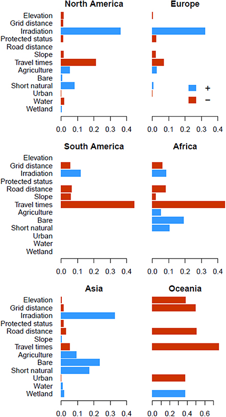
Figure 2. Relative determinant importance for each continent, computed as 1—Spearman rank correlation coefficient of the original model prediction with one where the relevant determinant is randomized (see section 2.3). Higher values indicate larger importance. Some determinants are not present in the best model and are thus not given a relative importance. The colours indicate the sign of the model coefficient of each determinant, i.e. a positive (blue) or negative (red) relation with the response variable (probability of PV occurrence). For land cover, the coefficients are relative to forest (which is in the intercept of the models). Note that for Oceania the x-axis is on a different scale.
Download figure:
Standard image High-resolution imageOverall, larger travel times to the nearest settlements (a proxy for electricity demand) and larger distances to infrastructure (roads and electricity grids) decrease the probability of PV occurrence, as indicated by negative coefficients (figure 2). With increasing distance to infrastructure and demand, the probability of PV occurrence drops quickly (figure 3). The probability increases more smoothly with increasing irradiation. Considering land cover types, PV facilities are more likely found in areas where agriculture, short natural vegetation or bare land prevail, but in our regression model land cover types are typically less important for the distribution of PV facilities than irradiation or travel time.
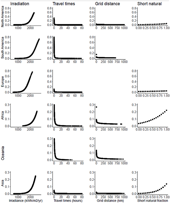
Figure 3. Partial dependency plots of important determinants (irradiation, travel times, grid distance and fraction of short natural vegetation,) for all considered continents. Partial dependence is computed by predicting the probability of occurrence (y-axis) with all determinants set to their mean value except for the determinant of interest (units of which are on the x-axis). For the purpose of this figure we ignore the spatial random effects when making predictions.
Download figure:
Standard image High-resolution image3.2. Probability maps
Our spatial predictions show how the probability of PV occurrence varies across the considered continents. In North America, the probability of PV occurrence is high across the south and south-west, where irradiation is high, travel times are low and short natural vegetation prevails. In northern U.S.A. and southern Canada, probabilities are high in regions where agriculture is abundant and travel times are low. In the South-East, higher irradiation and low travel times also result in high predicted probabilities (figure 4). Northern regions show a low probability, likely related to low irradiation and large distances to infrastructure and demand. In Europe, there are clear inter-country differences in probability of PV occurrence, and the increased probability towards the south within countries is explained by irradiation. In Africa and South America, the predicted probability of PV occurrence is visibly driven by (distance to) infrastructure and demand (figure 4). In Africa, probability of occurrence is slightly higher in certain countries such as South Africa, Algeria and Egypt.
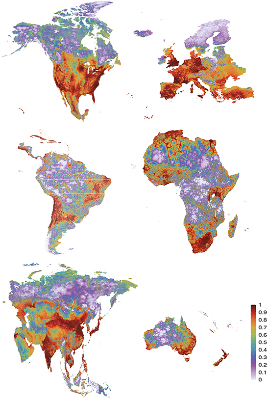
Figure 4. Ranked probability of PV occurrence based on our full mixed effect regression models at 0.011° resolution. Per continent the grid cell with the highest probability is given a value of 1, the grid cell with the lowest probability a value of 0.
Download figure:
Standard image High-resolution imageIn Asia, hotspots for PV occurrence are India and parts of China, as well as Japan, Thailand, and the Philippines. Hotspots also occur on the Arabian Peninsula, but overall the probability of occurrence (PoO) there is lower than one might expect given its high irradiation. Hence, in Asia, the inter-country differences stand out (see also table 2). Furthermore, PoO is high in the region east and north of the Caspian Sea, where agriculture and short natural vegetation prevail. In Oceania, PoO is high where demand is high and infrastructure is near. The importance of travel times, grid and road distance result in high PoO in New Zealand despite no PV facilities there in our data.
3.3. Comparison to integrated assessment model COE maps
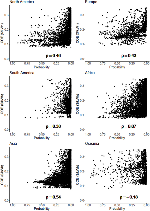
We found mostly positive correlations between the complement of PV occurrence probability and the COE, i.e. COE increases with decreasing probability of occurrence (PoO), except for Oceania (figure 5). Correlations range from −0.18 for Oceania to 0.54 for Asia. The relatively low value for South-America compared to North America, Europe and Asia may reflect mismatches in the Amazon, where forest is excluded from PV deployment in IMAGE (table S4, figure S19), while our predicted PoO is high in gridcells near infrastructure and demand. Also, PoO is high in northern Chile and the altiplano, where IMAGE assumes high COE. Also in Europe certain areas are excluded by IMAGE due to land cover constraints (table S4) while we predict high probability of occurrence, for instance in the United Kingdom, Germany or southern France. In Asia, there is a better match between COE and (the complement of) PoO. For instance, over the Arabian Peninsula, COE is low, but PoO is low as well due to low numbers of PV facilities in the region. In Africa the correlation is low, indicating mismatches between our PoO and IMAGE's COE. This could be related to high PoO in parts of western and eastern Africa, where COE is high. In Oceania we found a small, but negative correlation, indicating COE increases with increasing PoO. This could reflect that IMAGE excludes regions along the forested southeastern coast of Australia (SI figure S19), where PV facilities are present (SI figure S6) and our model predicts high PoO due to the proximity to settlements and infrastructure.
Figure 5. 1-PoO (probability of occurrence, bilinearly resampled to 0.5°, x-axes) versus COE (cost of electricity, $/kWh, y-axis) per continent. The Spearman rank correlation is given by ρ. For plotting purposes, the y-axis limit is set to 0.35 $/kWh but the full range of COE is included in the computation of ρ. SI figure S13 shows the spatial distribution of COE. Grid cells excluded from PV deployment in IMAGE are assigned the maximum COE within the continent +1 $/kWh.
Download figure:
Standard image High-resolution image
4. Discussion
4.1. Determinants of utility-scale PV distribution
We built regression models of the probability of PV occurrence using potential determinants derived from literature. We found that irradiation and travel times to the nearest settlement are the most important determinants, with probability of PV occurrence decreasing with longer travel times and increasing with higher irradiation. To a lesser degree, distance to the electricity grid and roads negatively affect probability of PV occurrence. This confirms the findings of other studies (e.g. Hernandez et al 2015, Al Garni and Awasthi 2017, Aly et al 2017, Oakleaf et al 2019, Tröndle et al 2019, Dupont et al 2020, Thormeyer et al 2020, Agyekum et al 2021, Balta-Ozkan et al 2021, Dunnett et al 2022). Other determinants such as elevation, protected status and slope show a negative impact on probability of PV occurrence, as also shown or assumed by others (Hernandez et al 2015, Al Garni and Awasthi 2017, Aly et al 2017, Oakleaf et al 2019, Tröndle et al 2019, Dupont et al 2020, Ouchani et al 2021), Agyekum et al 2021, Dunnett et al 2022), but they do not explain a large part of the distribution according to our regression models. We note, however, that at the smaller scales considered in most of the referenced literature, the relative importance of the determinants may shift. Compared to the sub-continental random-forest empirical approach of Dunnett et al (2022), we draw similar conclusions regarding the importance of travel times (accessibility), with irradiation and road distance coming second in their study.
Studies on the distribution of PV facilities or PV potential furthermore often include land cover, but our study suggests that land cover type is not an important determinant of the current PV distribution, in line with Dunnett et al (2022). Kruitwagen et al (2021) also indicate that land cover is not the single driving factor of PV siting decisions. For Africa and Asia, however, we found that higher fractions of agriculture, bare land or short natural vegetation are associated with a higher probability of PV occurrence compared to other land cover types, such as urban areas and water, which is in agreement with e.g. Hernandez et al (2015) and Dupont et al (2020). Other studies, however, often exclude agricultural areas in their a-priori PV potential assessment (Aly et al 2017, Tröndle et al 2019, Agyekum et al 2021) because of potential land-use conflicts. In their empirical regression of small-scale PV occurrence in Switzerland, Thormeyer et al (2020) show a positive correlation between agriculture and the number of PV projects, thus showing that, in reality, the presence of agriculture is a positive indicator of PV occurrence. Hernandez et al (2015) and Kruitwagen et al (2021) also show that PV facilities do occur in agricultural areas. Kruitwagen et al (2021) suggest that the presence of PV facilities in agricultural areas might be driven by the proximity to settlements and thus infrastructure, rather than the suitability of agricultural land itself. We note that our conclusions could be affected by the use of aggregated land cover fractions, we did not determine exactly what land cover or land use is displaced by PV facilities. The latter could be included in future studies by using inventories such as that of Kruitwagen et al (2021) and land cover products of higher resolution (∼10 m, such as Brown et al 2022). This would also allow to differentiate land cover preferences of different sizes of PV facilities (Kruitwagen et al 2021), which we did not consider.
In Europe and Asia, stronger differences between countries appear, possibly related to inter-country differences in e.g. climate policies. In the Americas and Oceania, inter-country differences are not apparent, which could be related to the smaller number of countries in these continents compared to Europe and Asia. Studies on smaller scales have indicated the importance of socio-economic and political aspects for the distribution of PV (e.g. Thormeyer et al 2020, Balta-Ozkan et al 2021). Here, we assumed that these aspects were covered by the random country and spatial effects in absence of indicators available at the global scale.
4.2. Theory vs practice: suggestions for integrated assessment models
Our regression model provides insights into the global expansion of PV facilities, which is relevant for tools exploring long-term energy scenarios, such as econometric analyses or IAMs. The comparison of our empirically-derived probability of occurrence maps to the production cost (COE) maps of the IMAGE IAM reveal correlations between −0.18 and 0.54.
It is, however, critically important to realize the conceptual differences between the empirically-derived probability maps based on the current situation, and the PV potential calculations as done by IMAGE. IMAGE identifies potentially attractive areas for PV deployment rather than predict where PV will be deployed in the short term. This means that for instance current national barriers or support for PV deployment are not taken into account, as this would prevent IAMs from identifying potentially attractive sites in case of changes in policy. The same argument could apply to the exclusion of land-use categories, such as (the majority of) agricultural areas, as PV locations, as in IAMs that would automatically lead to a reallocation of current land use.
For instance, in IMAGE, a large number of grid cells is excluded when computing the geographical potential based on land cover and topography (see table S3, figure S19). However, some excluded regions have a high probability of PV occurrence according to our regression models, resulting in a mismatch between COE and probability of occurrence. This could partly be due to country-scale policies, such as in Germany or the UK, where the number of PV facilities is high and, therefore, our results show a high probability of occurrence.
Overall, our regression models do support the underlying assumptions for the geographical potential made in IMAGE and PV potential studies (e.g. Dupont et al 2020, Gernaat et al 2021, see also section 4.1): land cover types such as agriculture, short natural vegetation and bare areas (incl. deserts) are positive determinants of PV occurrence compared to forests, and IMAGE assumes that grid cells with such land cover types are (partly) available for PV deployment. IMAGE excludes urban areas, high altitudes and protected areas, for which we find negative coefficients in our regression models. We cannot assess whether the exact suitability factors assigned in IMAGE (SI table S4) match the actual distribution of PV facilities because we aggregated the land cover types to fractions. So, for instance, in North America, 40% of PV facilities are in grid cells where >50% of the land cover is agriculture, but we cannot confirm whether those are positioned upon agricultural land, or near.
Furthermore, we find that proximity to demand (travel times) is an important determinant, with probability of PV occurrence decreasing with increasing travel times (accessibility) and to a lesser extent with increasing distance to roads and electricity grids. In the IMAGE COE maps, the proximity to infrastructure and demand is included indirectly by including transmission costs per km of distance to load centres (SI text 4). Previous assessments with IMAGE did not include transmission costs and excluded agricultural land from PV deployment (e.g. Köberle et al 2015); according to our regression model, it is thus an improvement that these are now included (e.g. Gernaat et al 2021).
It should also be noted that we computed the probability of occurrence at a much higher resolution than that of the PV cost and potential maps in IMAGE (0.011° vs 0.5°) and IMAGE assigns one land cover type to each 0.5° grid cell. Using land cover fractions (as in our determinants) or moving to higher-resolution maps would make the IAM's potential and production cost maps, and therefore also the energy scenarios at aggregated scales, more realistic. Higher-resolution maps would also better represent topographic determinants (slope and elevation), and thus in the end create more realistic cost-supply curves. This could improve scenarios of PV deployment on which policymakers can act (Creutzig et al 2017).
5. Conclusions
We were able to explain the distribution of utility-scale PV facilities across the globe with relatively high accuracy, using a suite of relevant determinants (distance to roads and electricity grid, travel time, slope, elevation, protected status, irradiation, and land cover types). Travel time as well as irradiation are the most important determinants overall. Especially, especially in Europe and Asia, other factors play a role as well, possibly related to inter-country differences in socio-economic and political factors.
These insights into the global expansion of PV facilities are useful for tools exploring energy scenarios, such as econometric analyses and IAMs. The correlation of our probability of occurrence maps to PV production cost in the IMAGE IAM reveals that as probability of occurrence increases, costs (per kWh) decrease, except for Oceania. However, the correlation is not strong, which could be related to the conceptual differences between probability maps and production cost maps. Our regression model results do support the underlying assumptions used when creating the IAM PV geopotential. Lastly, we suggest that using higher-resolution maps in IAM potential and production cost computations may improve PV deployment scenarios upon which policymakers act.
Acknowledgments
This work is part of Grant 016.Vici.170.190, financed by the Netherlands Organisation for Scientific Research (NWO). NWO had no role in this study's design. We thank Jelle Hilbers for help computing distances to the electricity grid. We furthermore thank the referees and editors for their constructive remarks on this manuscript.
Data availability statement
The Wiki-Solar dataset is proprietary and can be obtained through wiki-solar.org. Other data sources are referenced in table 1. IMAGE data can be downloaded following information provided in Gernaat et al (2021). Code used to process data, create the regression models, and the comparisons are available through GitHub: https://github.com/JoyceBosmans/Scripts_PV_determinants.
The data generated and/or analysed during the current study are not publicly available for legal/ethical reasons but are available from the corresponding author on reasonable request.
Conflict of interest
We declare that none of the authors have a conflict of interest.
Footnotes
- 4
Floating PV makes up <0.5% of the dataset.
- 5
We used layer 12, travel_time_to_cities_12.tif.
- 6
Based on the 7982 current PV facilities for which we computed total panel area in Bosmans et al (2021), we find that only 151 (<2%) have a surface area of more than 1.08 km2 (the average land grid cell area at 0.011°). At ESA CCI's 300 m resolution, 3614 facilities (45%) would cover multiple grid cells. Note that we only consider panel area and made no assumption on packing factors/area of the entire facility.
Supplementary data (5.2 MB PDF)