

Abstract
The heat index, or apparent temperature, was never defined for extreme heat and humidity, leading to the widespread adoption of a polynomial extrapolation designed by the United States National Weather Service. Recently, however, the heat index has been extended to all combinations of temperature and humidity, presenting an opportunity to reassess past heat waves. Here, three-hourly temperature and humidity are used to evaluate the extended heat index over the contiguous United States during the years 1984–2020. It is found that the 99.9th percentile of the daily maximum heat index is highest over the Midwest. Identifying and ranking heat waves by the spatially integrated exceedance of that percentile, the Midwest once again stands out as home to the most extreme heat waves, including the top-ranked July 2011 and July 1995 heat waves. The extended heat index can also be used to evaluate the physiological stress induced by heat and humidity. It is found that the most extreme Midwest heat waves tax the cardiovascular system with a skin blood flow that is elevated severalfold, approaching the physiological limit. These effects are not captured by the National Weather Service's polynomial extrapolation, which also underestimates the heat index by as much as 10 ∘C (20 ∘F) during severe heat waves.
Export citation and abstract BibTeX RIS
1. Introduction
Among meteorological phenomena, heat waves are the number one cause of death in the United States (Changnon et al 1996). Heat waves pose a particular threat to the elderly (Carleton et al 2020), those without access to air conditioning (O'Neill et al 2005), and outdoors workers (Acharya et al 2018). As the Earth warms, the frequency and severity of heat waves is expected to increase (Dosio et al 2018). It is important, therefore, to have accurate metrics for heat waves, both to issue operational warnings and to plan adaptations for the future.
Many different metrics have been used to define, identify, and measure heat waves (Xu et al 2016). Defined as having an anomalously high air temperature, heat waves in the contiguous United States (CONUS) are found to be most severe in the South (Meehl and Tebaldi 2004, Dosio et al 2018). Heat waves have also been defined using the heat index, also known as the apparent temperature, which is a metric that maps one-to-one onto physiological states (different rates of skin blood flow) in hot conditions (Steadman 1979). Most studies that define heat waves in terms of the heat index also find that the frequency of heat waves peaks in the South (e.g. Smith et al 2013, Lyon and Barnston 2017). An exception is the study of Robinson (2001), who found that heat waves are comparably frequent in the South, Midwest, and Mid-Atlantic.
It is notable, however, that these studies—and all other studies that have used Steadman's heat index to study heat waves—have used not the actual heat index, but a functional approximation to the heat index. Of the many different approximations (Anderson et al 2013), the most widely used is the polynomial fit developed by the United States National Weather Service (Rothfusz 1990, National Weather Service 2014). The National Weather Service (NWS) approximation is used on a regular basis to issue warnings to the public and to study past severe heat (e.g. Robinson 2001, Kim et al 2006, Yip et al 2008, Smith et al 2013, Lyon and Barnston 2017, Tustin et al 2018, Xie et al 2018, Perera et al 2022) and future severe heat (e.g. Delworth et al 1999, Diffenbaugh et al 2007, Opitz-Stapleton et al 2016, Diem et al 2017, Modarres et al 2018, Dahl et al 2019, Rao et al 2020, Rahman et al 2021, Amnuaylojaroen et al 2022). Even in the current climate, there are conditions hotter and more humid than were considered and tabulated by Steadman (1979), and so the NWS approximation is used to extrapolate the heat index beyond those tabulated values. That extrapolation is used extensively in operational warnings and in the aforementioned research studies.
From the perspective of social impacts, heat waves would ideally be identified and quantified using not an extrapolation but an accurate measure of physiological stress. Recently, Lu and Romps (2022) extended Steadman's heat index to all combinations of temperature and humidity, providing such a measure. The objectives of this paper are threefold: (a) to use the extended heat index to define and rank the most severe heat waves experienced over the United States during recent decades, (b) to evaluate the extent to which the NWS approximation errs in reporting the heat index during those heat waves, and (c) to evaluate the physiological state required of humans exposed to conditions during the most severe of those heat waves.
2. The heat index
To motivate the use of the heat index, we give here a brief review. As is well known, sweating is a physiological adaptation to high temperatures, with the evaporation of sweat providing a cooling effect. But this adaptation has limits: if the air is sufficiently hot and humid, evaporative cooling is unable to compensate for the inputs of metabolic heat, sensible heat, and infrared radiation, and the core temperature rises. In general, in hot and humid conditions, humans are subjected to greater physiological stress if either the temperature or humidity increases.
To capture these effects, Steadman (1979) developed a model of thermoregulation with parameters chosen to represent a healthy adult walking in the shade with ample access to drinking water. The model quantifies the behavior (clothing thickness) and physiology (skin blood flow) in response to a combination of temperature and humidity. An important aspect of this model is that the human responds to changes in temperature and humidity by adjusting only one parameter at a time. For example, in relatively cold conditions, the human responds to changes in temperature by adjusting the thickness of the clothing being worn. Once that response has been exhausted (i.e. the clothing thickness has been driven to zero), the human responds by adjusting its skin blood flow. As a consequence, all states form a one-dimensional family, i.e. the states can be parameterized by a single variable. For example, in the original Steadman model, the states could be parameterized by ζ with the clothing thickness in millimeteres equal to  for ζ < 0 and the skin blood flow, in liters per minute, elevated by an amount of ζ for
  .
.
Since the space of states is one-dimensional, whereas the space of all possible temperature and humidity is two-dimensional, each state corresponds to a one-dimensional isopleth in temperature-humidity space. For example, all pairs of temperature and humidity corresponding to a clothing thickness of five millimeters form a continuous one-dimensional curve with  . So long as the actual air temperature and humidity remain on an isopleth, a human's experience of those conditions does not change (e.g. the choice of clothing or the skin blood flow remains the same). The heat index, which is a function of temperature and humidity, is simply a convention for assigning a unique temperature to each isopleth: the heat index is defined to be the temperature of the isopleth at 1600 Pa (Steadman 1979).
For illustration, figure 1 shows the curve corresponding to ζ = 0.88 (the state with an extra 0.88 l min−1 of skin blood flow), which intercepts a vapor pressure of 1600 Pa at a temperature of 60 ∘C (140 ∘F). All pairs of temperature and humidity lying on this curve have a heat index of 60 ∘C and induce identical behavioral and physiological responses (minimization of clothing and an extra skin blood flow of 0.88 l min−1). In this way, every pair of temperature and humidity can be mapped to a value of the heat index and a thermoregulatory state. This is useful for communicating the hazard posed by high heat and humidity. For example, a heat index of 60 ∘C (140 ∘F) corresponds to a skin blood flow that is about two and a half times its value at room temperature. Maintaining a high skin blood flow can stress the cardiovascular system, even leading to death by heart failure. On the other hand, failing to maintain the required skin blood flow would lead to an elevated core temperature, which, if elevated by only a few degrees, can lead to death by hyperthermia.
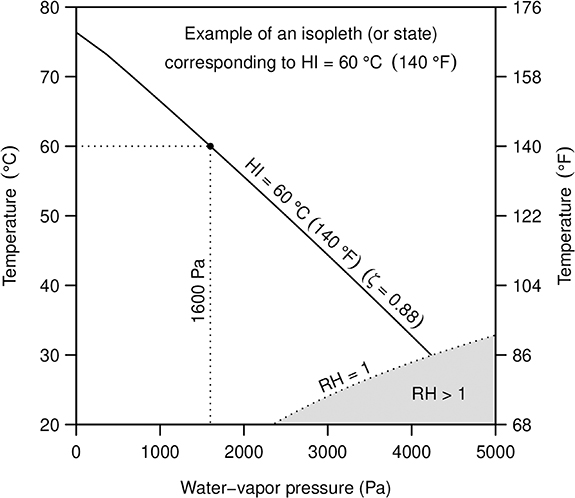
Figure 1. The curve, in temperature-humidity space, corresponding to the state with an extra 0.88 liters per minute of skin blood flow. The small circle indicates where the curve intercepts the reference vapor pressure of 1600 Pa. The temperature of that point is 60 ∘C (140 ∘F), which defines the heat index (HI) for all points on the curve.
Download figure:
Standard image High-resolution imageUnfortunately, the heat index defined by Steadman (1979) was defined only up to certain combinations of heat and humidity, beyond which the heat index was undefined. Those originally undefined regions are labeled V and VI in figure 8 of Lu and Romps (2022). For example, Steadman was unable to define the heat index for 30 ∘C (86 ∘F) at 90% relative humidity, or for 35 ∘C (95 ∘F) at 65% relative humidity. The heat index was left undefined in those conditions due to an apparent failure of the underlying model of thermoregulation: the vapor pressure at the skin surface exceeded the saturation value. To allow for extrapolation beyond this point of apparent failure, the NWS developed and adopted a polynomial fit to the heat index as a function of temperature and humidity (Rothfusz 1990, National Weather Service 2014). But without a model of thermoregulation at the high values of temperature and humidity, those extrapolated values have no interpretation with respect to a thermoregulatory state. Furthermore, as will be shown below, the extrapolated values used by the NWS are biased low by ∼10 ∘C (∼20 ∘F) during the peaks of severe heat waves.
Recently, Lu and Romps (2022) showed that Steadman's model, and therefore the heat index, could be extended in a physical way. One of the keys to extending the model to high heat and humidity is to allow sweat to drip off the skin; this simple fix avoids any water-vapor supersaturation. This extension is backwards compatible—it gives the same values as the model of Steadman (1979) where the original model was defined—but extends the definition of the heat index to all combinations of temperature and humidity. And, as with the original heat index, every value maps one-to-one to a one-dimensional family of thermoregulatory states, which are parameterized by the fraction of skin covered by clothing in very cold conditions, the thickness of clothing in cold-to-mild conditions, the skin blood flow in hot conditions, and the rate of core-temperature rise in dangerously hot or lethal conditions.
3. Methods
To calculate the heat index (HI), we use the instantaneous two-meter temperature and humidity from the National Centers for Environmental Prediction (NCEP) North American Regional Reanalysis (NARR; Mesinger et al
2006), which provides data at a grid spacing of 32 km every three hours. We calculate the extended heat index (Lu and Romps 2022) for each three hourly snapshot from 1 January 1984 to 31 December 2020. We also calculate the polynomial fit to the heat index developed by the National Weather Service (Rothfusz 1990, National Weather Service 2014) with one minor modification made here to avoid bad behavior at cold temperatures (see the
We will identify and quantify heat waves using the spatially integrated exceedance of the daily maximum heat index beyond its local 99.9th percentile of daily maxima. This choice defines heat waves in terms of their severity as perceived by humans, although there are other choices that could be made (e.g. weighting the exceedance by population density). The 99.9th percentile is chosen to isolate the most extreme events, i.e. those events comprised of values with a ∼3 year (1000 day) return period.
We first define a grid cell's daily maximum heat index HI as the highest HI among UTC 12, 15, 18, and 21 on the same date and UTC 0, 3, 6, and 9 of the following day. During spring, summer, and early fall, when CONUS is observing daylight saving, this captures all available NARR data from 5am to 2am (next day) local time on the West Coast and 8am to 5am (next day) local time on the East Coast. With 37 years of data, this gives 13 515 daily maximum values. The next step is to calculate, separately for each grid cell, the 99.9th percentile of HI
 over all 13 515 days, which we denote by HI99.9.
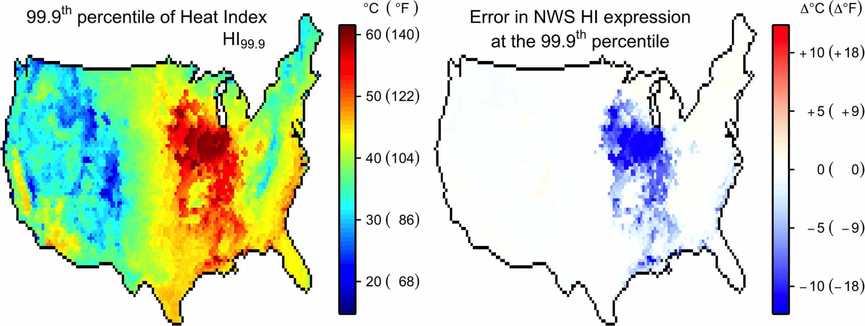
The map of HI99.9 is shown in the left panel of figure 2. We see that the most extreme values of the heat index do not occur in the South as one might expect, but in the Midwestern states of Illinois, Iowa, and Missouri. In those states, the 99.9th percentile of the daily maximum heat index reaches up to and beyond 60 ∘C (140 ∘F). As seen in the right panel of figure 2, these extreme values are not captured by the polynomial extrapolation used by the NWS. In those midwestern states, the 99.9th percentile is underestimated by the NWS polynomial by as much as ∼10 ∘C (∼20 ∘F).
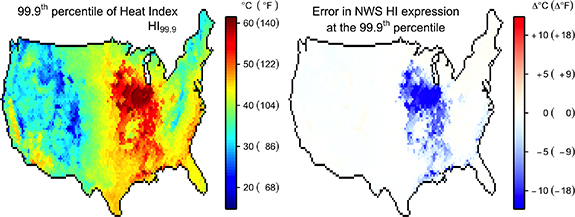
Figure 2. (Left) The 99.9th percentile of the daily maximum heat index HI99.9. (Right) The 99.9th percentile of the daily maximum heat index calculated by the NWS approximation minus the actual HI99.9.
Download figure:
Standard image High-resolution imageTo prepare to identify heat waves, we first calculate the daily time series of the integral over CONUS of the number of degrees that HI is in excess of the 99.9th percentile,
where x and y denote east–west and north–south distance and d denotes the day. This time series has 13 515 values: one for each day from 1 January 1984 to 31 December 2020. To find the first heat wave, we identify the maximum value in this time series. To find the start and end of that heat wave, we find the largest contiguous interval in that time series containing that maximum for which all values are at least 25% as large as that maximum; this defines the heat wave. We then find the two nearest local minima that bracket that heat wave and set to zero the interval that starts and ends with those two local minima. We then repeat the process to find the second heat wave, and so on. This identifies heat waves naturally ranked by the peak of their area-integrated exceedance of HI99.9. The sensitivity of this ranking to the threshold, chosen here to be 25%, is explored in figures S1 and S2. A lower threshold would result in longer-duration heat waves, but would not substantially alter the ranking of the most severe heat waves: for threshold values ranging from 4% to 34%, the ranking of the top five heat waves is unchanged.
4. Results
For visualization of a heat wave, we define HI for each grid cell as the largest HI
 in that grid cell during the days of the heat wave. For each of the top nine heat waves identified by the algorithm described above, figure 3 displays HI
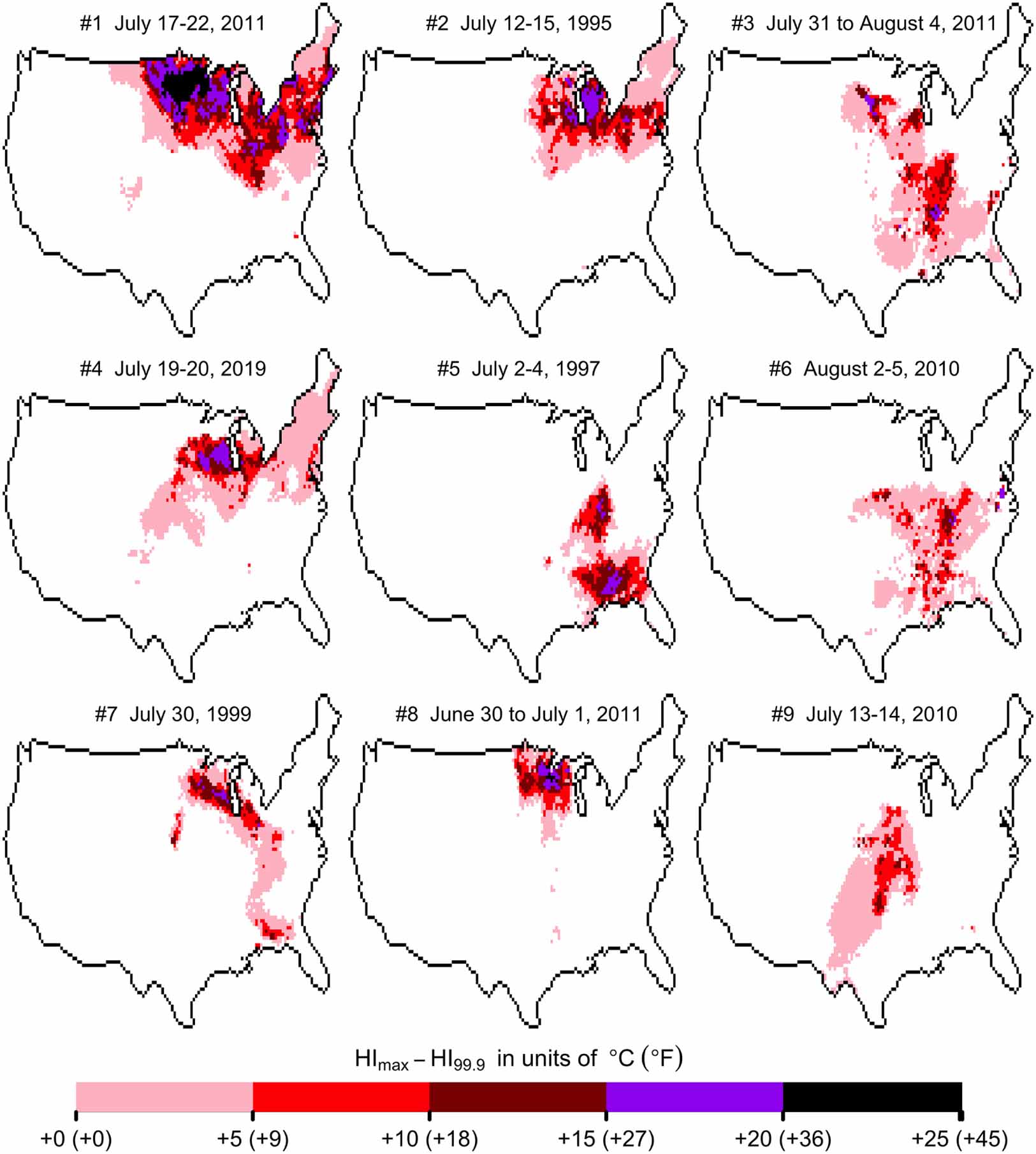
 minus HI99.9. The most severe heat wave (heat wave #1) is found to be centered on the Midwest during 17–22 July 2011. This time and place corresponds to a heat wave that generated a raft of news coverage and a dramatic spike in heat-related illness (Storm and Fowler 2011, Berry et al
2013, Fuhrmann et al
2016). The second most severe heat wave (heat wave #2) is identified as occurring over the same region during 12–15 July 1995. This again corresponds to a well-known heat wave that hit the city of Chicago especially hard, leading to hundreds of heat-related deaths (Semenza et al
1996, 1999, Whitman et al
1997, Dematte et al
1998). A list of the top 20 heat waves is given in table 1. Although the Midwest occupies only 26% of the area of the contiguous United States, it contains the peak heat index during 7 of the top 10 heat waves. This is particularly notable in comparison to the South, which occupies 29% of the area, but contains the peak heat index during only 3 of the top 10 heat waves. A list of the top 100 heat waves identified by this algorithm is given in tables S1 and S2 and maps of their
minus HI99.9. The most severe heat wave (heat wave #1) is found to be centered on the Midwest during 17–22 July 2011. This time and place corresponds to a heat wave that generated a raft of news coverage and a dramatic spike in heat-related illness (Storm and Fowler 2011, Berry et al
2013, Fuhrmann et al
2016). The second most severe heat wave (heat wave #2) is identified as occurring over the same region during 12–15 July 1995. This again corresponds to a well-known heat wave that hit the city of Chicago especially hard, leading to hundreds of heat-related deaths (Semenza et al
1996, 1999, Whitman et al
1997, Dematte et al
1998). A list of the top 20 heat waves is given in table 1. Although the Midwest occupies only 26% of the area of the contiguous United States, it contains the peak heat index during 7 of the top 10 heat waves. This is particularly notable in comparison to the South, which occupies 29% of the area, but contains the peak heat index during only 3 of the top 10 heat waves. A list of the top 100 heat waves identified by this algorithm is given in tables S1 and S2 and maps of their  are shown in figure S3.

Figure 3. The top nine heat waves from 1 January 1984 to 31 December 2020 as identified using the spatially integrated map of HI99.9 exceedance.
Download figure:
Standard image High-resolution imageTable 1. Top 20 most severe CONUS heat waves from 1984 to 2020.
| Rank | Dates | State with max HI | Max HI in ∘C (∘F) | Max NWS value in ∘C (∘F) |
|---|---|---|---|---|
| 1 | 17–22 July 2011 | North Dakota | 70 (157) | 59 (139) |
| 2 | 12–15 July 1995 | Illinois | 68 (154) | 57 (135) |
| 3 | 31 July–4 August 2011 | Mississippi | 70 (158) | 59 (139) |
| 4 | 19–20 July 2019 | Iowa | 68 (155) | 58 (136) |
| 5 | 2–4 July 1997 | Alabama | 63 (145) | 51 (124) |
| 6 | 2–5 August 2010 | Iowa | 65 (149) | 54 (129) |
| 7 | 30 July 1999 | Wisconsin | 63 (146) | 51 (124) |
| 8 | 30 June–1 July 2011 | Wisconsin | 66 (150) | 54 (129) |
| 9 | 13–14 July 2010 | Iowa | 65 (149) | 53 (127) |
| 10 | 23–27 July 2005 | Mississippi | 61 (141) | 50 (121) |
| 11 | 10–11 July 2011 | Indiana | 64 (147) | 52 (126) |
| 12 | 1–3 July 2002 | Maine | 61 (141) | 48 (119) |
| 13 | 11–16 August 2010 | Illinois | 64 (147) | 52 (126) |
| 14 | 10–14 July 2002 | Kentucky | 47 (117) | 43 (109) |
| 15 | 01 July 2012 | South Carolina | 69 (155) | 57 (135) |
| 16 | 1–2 July 2020 | Oklahoma | 62 (144) | 51 (125) |
| 17 | 13–15 July 2015 | Tennessee | 65 (149) | 52 (126) |
| 18 | 12–14 August 2019 | Louisiana | 61 (143) | 49 (120) |
| 19 | 30 June–3 July 2018 | Texas | 59 (139) | 46 (114) |
| 20 | 30 July–3 August 2006 | Illinois | 62 (144) | 51 (123) |
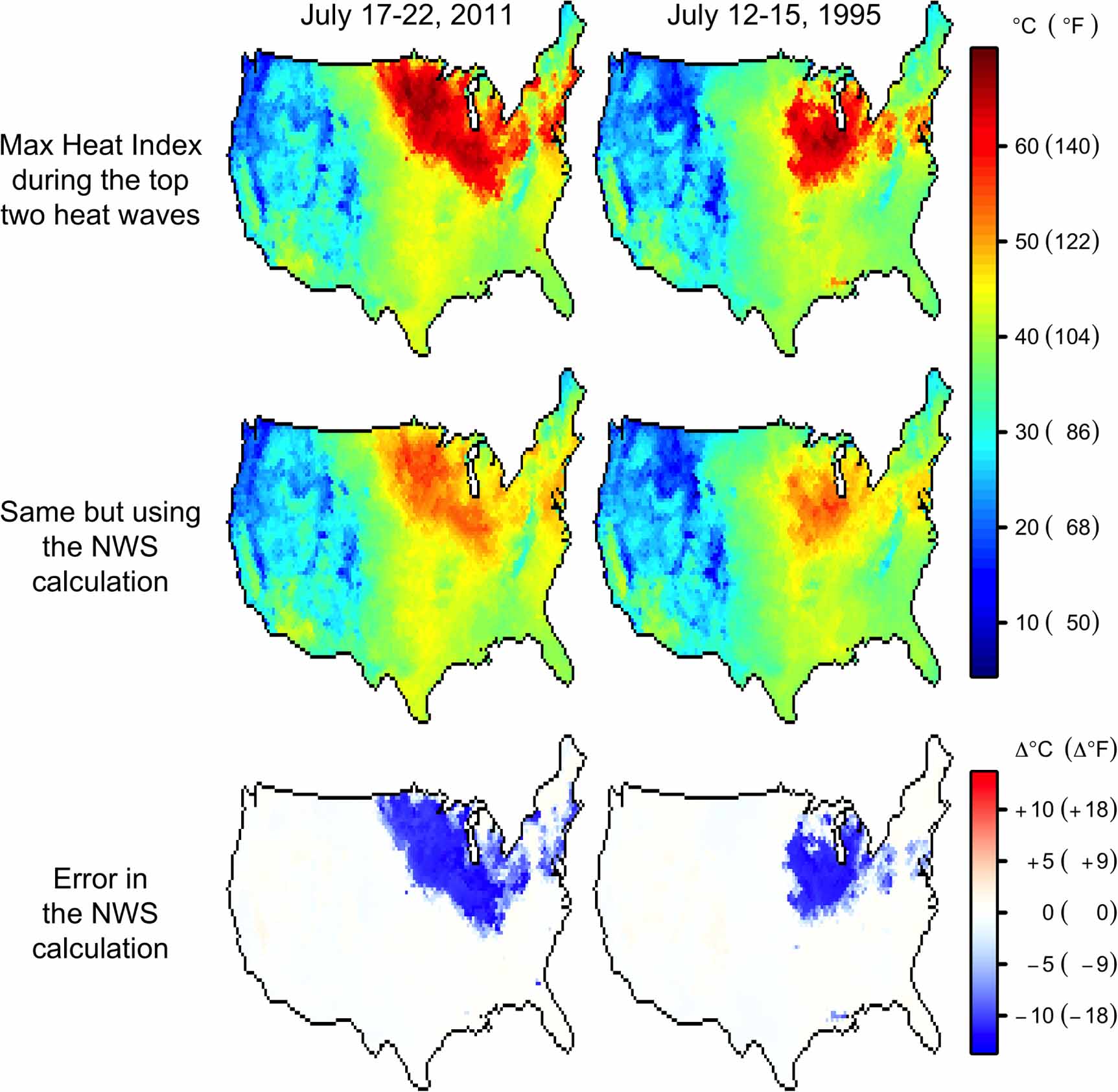
The top row of figure 4 displays HI during the top two heat waves. In both cases, the heat index reaches values well in excess of 60 ∘C (140 ∘F), reaching 70 ∘C (157 ∘F) during the 2011 heat wave and 68 ∘C (154 ∘F) during the 1995 heat wave. Compared to
  , HI
, HI is more tightly peaked in the Midwest with typical values of ∼130 ∘F–150 ∘F. Since Steadman's original model fails for such high heat and humidity, the NWS has used its polynomial fit to report a heat index by extrapolation. The values resulting from that extrapolation are shown in the middle row of figure 4. The peak values of the heat index are noticeably muted in the NWS extrapolation. The error in the NWS extrapolation, shown in the bottom row of figure 4, is ∼10 ∘C (∼20 ∘F) for the peak values of the heat index.

Figure 4. (Top) Actual HI for the top two heat waves. (Middle) The HI
 according to the NWS approximation. (Bottom) The error in the NWS approximation.
Download figure:
Standard image High-resolution imageDuring the July 1995 heat wave, the NWS reported a peak heat index of 119 ∘F at O'Hare airport and 125 ∘F at Midway airport. Those values were subsequently referenced by major newspapers (Kaye 1995, Lev and Ryan 1995, Nathans 1995, Stein and Kaplan 1995), the Centers for Disease Control and Prevention (1995), CDC, and research studies (Whitman et al 1997, Dematte et al 1998, Semenza et al 1999, Grady 2013). Using the hourly temperature and relative humidity recorded at O'Hare and Midway, we find that the NWS extrapolation yields a peak HI of 118 ∘F at O'Hare airport at 1pm local time (when the temperature was 100 F and the relative humidity was 50%) and 124 ∘F at Midway airport at 12pm (temperature of 100 F and relative humidity of 55%), consistent with the reported values. Using these same temperature and humidity values, we can calculate the actual heat index to have been 123 ∘F at O'Hare (5 ∘F higher than reported by the NWS) and 141 ∘F at Midway (17 ∘F higher than reported by the NWS).
Like the original heat index, each value of the extended heat index maps one-to-one to thermoregulatory states (Lu and Romps 2022). For the extreme HI values in the Midwest during the July 2011 and July 1995 heat waves, a healthy adult walking in the shade would have been stressed physiologically in an effort to maintain a healthy core temperature: their body would need to sweat profusely (dripping sweat) and maintain a rapid rate of blood flow to the skin. This high blood flow would be needed to maintain an elevated skin temperature to ensure that the skin loses net energy to the environment at the same rate that metabolic heat is added to the core.
The right column of figure 5 shows the skin blood flow required to maintain a healthy core temperature at the times of the maximum heat index during the top two heat waves. Combining the model of Steadman (1979) with the skin blood flow relation from Gagge et al (1972) (see Lu and Romps 2022), the normal skin blood flow (i.e. in mild conditions) is 0.57 l min−1. Therefore, the dark red colors in figure 5 correspond to skin blood flows that are severalfold higher than usual, indicating a high state of physiological stress. The highest rate of skin blood flow measured in the laboratory, achieved by inducing severe thermal stress, is estimated to be around 7.8 l min−1 (Rowell 1974, Simmons et al 2011). In the 2011 heat wave, there are a handful of grid cells of the reanalysis that report a required skin blood flow approaching 7.8 l min−1 and one grid cell that exceeds that value. In contrast, the required skin blood flow implied by the NWS approximation to the heat index, shown in the left column of figure 5, never exceeds 1.3 l min−1 during either heat wave.

Figure 5. The maximum skin blood flow required to maintain a healthy core temperature during the heat waves of (top) 17–22 July 2011 and (bottom) 12–15 July 1995 as calculated using the National Weather Service's approximation to the heat index (left) and the actual heat index (right). On the color bar, 'normal' corresponds to 0.57 l min−1, the resting value, and 'human limit' corresponds to 7.8 l min−1, the physiological limit estimated from laboratory experiments.
Download figure:
Standard image High-resolution image
5. Discussion
Using the heat index, which has recently been extended to high heat and humidity (Lu and Romps 2022), the most physiologically stressful heat waves in the contiguous United States occur most often in the Midwest, not in the South as might be expected or previously reported (e.g. Smith et al 2013, Lyon and Barnston 2017). The finding that the Midwest is home to the most hazardous heat and humidity is manifested both in the map of the 99.9th percentile of the daily maximum heat index HI99.9 (figure 2) and in the locations of the most severe heat waves as ranked by their exceedance of HI99.9 (figure 3). In both the July 1995 and July 2011 heat waves, the soils of the Midwest were moist when the high pressure arrived, trapping heat and humidity in a shallow boundary layer (Kunkel et al 1996, Moser 2011). Although the ingredients of individual events can be described in this way, we are not aware of any first-principles theory for why the most severe US heat waves tend to occur preferentially in the Midwest.
The calculation used by the US National Weather Service underestimates the apparent temperature in extreme heat waves by as much as twenty degrees Fahrenheit. This has real consequences for our understanding of physiological impacts. For example, during the July 1995 heat wave, the heat index at the Midway airport hit a high of 141 ∘F. In other words, conditions in the shade at the airport felt the same as being in a room at 141 ∘F with 1.6 kPa of water-vapor pressure (8% relative humidity at that temperature). The physiological consequence of this exposure is that the cardiovascular system must maintain a skin blood flow that is elevated by 170%. In contrast, the heat index of 124 ∘F calculated by the NWS would imply a skin blood flow that is elevated by only 90%. As seen in the reanalysis, the discrepancy was even larger elsewhere in Illinois during the July 1995 heat wave, with the required skin blood flow elevated by 120% according to the NWS approximation, but elevated by 820% according to the actual heat index. Thus, the approximate calculation used by the NWS, and widely adopted, inadvertently downplays the health risks of severe heat waves.
Acknowledgment
This work was supported by the U.S. Department of Energy's Atmospheric System Research program through the Office of Science's Biological and Environmental Research program under Contract DE-AC02-05CH11231.
Data availability statement
The data that support the findings of this study are openly available at the following URL/DOI: https://downloads.psl.noaa.gov/Datasets/NARR/monolevel/.
Conflict of interest
The authors declare no competing interests.
Appendix.: The NWS approximation
The NWS approximation to the heat index is
with
where  is the Heaviside unit step function and the variables T, RH, and HI in this expression are dimensionless: T is the temperature in degrees Fahrenheit, RH is the relative humidity in percent, and HI is the heat index in degrees Fahrenheit (Rothfusz 1990, National Weather Service 2014). In the NWS implementation, HI is set equal to X or Y depending on whether X is greater than or less than 80. That leads to some very bad behavior at low temperatures. For example, at 0 ∘C (32 ∘F) and 70% relative humidity, the heat index would be given as 74 ∘C (166 ∘F). To avoid this problem, we modify the NWS approximation to use T = 80 as the dividing line between these two expressions:
This eliminates the poor behavior at cooler temperatures and does not affect the performance of the approximation at warmer temperatures.
Supplementary data (0.5 MB PDF)