

Abstract
Annual and seasonal mean tropical and subtropical precipitation biases in present-day climate simulations by phase 6 of the Coupled Model Intercomparison Project (CMIP6) models are evaluated. We analyze 23 CMIP6 models, which are grouped into those without (NOS) and with (SON) falling ice (snow) radiative effects (FIREs). The SON group is further divided according to treatments of ice-cloud radiative properties with separate (SON2) and combined cloud ice and snow contents (SON1). SON2 mitigates precipitation bias drastically relative to NOS, but SON1 overestimates precipitation in the subtropics, which deteriorates its performance relative to SON2 and NOS. Large offsets between SON2 and SON1 and between SON and NOS contribute to the slight improvement of CMIP6 relative to CMIP5, largely due to the contribution of SON2. The different treatments of ice-cloud radiative properties between SON2 and SON1 seem to be potentially linked to differences in precipitation biases. Results suggest that further in-depth investigation of cloud ice–radiation–circulation interactions is required.
Export citation and abstract BibTeX RIS

Original content from this work may be used under the terms of the Creative Commons Attribution 4.0 license. Any further distribution of this work must maintain attribution to the author(s) and the title of the work, journal citation and DOI.
1. Introduction
Accurate simulations of tropical precipitation remain a challenge for global climate models such as those in the previous phase 5 of the Coupled Model Intercomparison Project (CMIP5; Taylor et al
2012) and current phase 6 (CMIP6; Eyring et al
2016). It is essential to evaluate the coupling among clouds, convection, precipitation and radiation in the present-day climate (historical run) simulations to ensure confidence in the fidelity of future climate projections (Flato et al
2013). However, from the infancy of coupled general circulation model (CGCM) development, most CGCMs share similar systematic biases, including a spurious double intertropical convergence zone (ITCZ) in both Pacific and Atlantic oceans with heavy rain parallel to the equator (e.g. Mechoso et al
1995, Lin 2007, Li and Xie 2014, Zhang et al
2015, Xiang et al
2017, Woelfle et al
2019, Tian and Dong 2020). The ITCZ is a band of heavy precipitation across the oceans near the equator associated with low-level convergence from the north and south. In observations, the ITCZ is found from  and there is no ITCZ or zonally oriented surface convergence zone over the southeastern Pacific or South Atlantic, except for a short period in March and April (e.g. Zhang 2001, Haffke et al
2016).
and there is no ITCZ or zonally oriented surface convergence zone over the southeastern Pacific or South Atlantic, except for a short period in March and April (e.g. Zhang 2001, Haffke et al
2016).
A recent study by Tian and Dong (2020) indicates that CMIP3's and CMIP5's double‐ITCZ bias persists in the latest CMIP6 models. In this study, we provide evidence that progress has been made in some subsets of CMIP6 models, which consider falling ice radiative effects (FIREs). These FIREs alter the column radiative heating rate profile, which may have a slight direct impact on surface precipitation, but most importantly, drives circulation changes in the trade wind regions through radiation–circulation coupling (Waliser et al 2009, 2011, Li et al 2012, 2013, 2014a, 2014b, Michibata et al 2019). The circulation change can influence tropical precipitation and thus the location of the ITCZ. In CMIP3 and CMIP5, most GCMs did not consider FIREs (Li et al 2012, 2013), but with CMIP6 more GCMs now include FIREs (Gettelman and Morrison 2015, Li et al 2020, Danabasoglu et al 2020). In this study, the progress in precipitation simulation from CMIP5 to CMIP6 over the tropical and subtropical Pacific and Atlantic oceans are examined by categorizing CMIP6 models into different groups according to treatments of cloud ice–radiation interactions. The Indian ocean is not examined, due to its strong seasonal reversal controlled by the thermal effect of the Tibetan Plateau (Abe et al 2013, He et al 2019).
The potential importance of FIREs has been studied in a number of studies (Waliser et al 2009, 2011, Gettelman and Morrison 2015, Li et al 2012, 2013, 2014a, 2014b; Michibata et al 2019). These studies showed a distinct Pacific Ocean pattern of radiation–circulation changes related to FIREs. This mechanism can be briefly described as follows. The inclusion of FIREs reduces upper-level outgoing longwave radiation and stablizes atmospheric columns over the ITCZ and South Pacific Convergence Zone (SPCZ; extending southeastward starting from the maritime continent), which leads to reduction of anomalous low-level outflows and surface wind stress, compared with the case when FIREs are excluded. This anomalous low-level outflow typically opposes the trade wind motion, so this reduction in outflow from the convective regions increases surface wind stress in the trade regions, leading to colder ocean temperatures on the flanks of the ITCZ and a reduced precipitation bias over the trade-wind regions.
This study uses 28 CMIP5 and 23 CMIP6 fully coupled GCMs with historical runs (supplementary information (SI) (available online at https://stacks.iop.org/ERL/15/124068/mmedia), table 1). Only 5 models consider FIREs in CMIP5 while 11 models consider FIREs (Snow ON or SON) and 12 models neglect FIREs (NO Snow or NOS) in CMIP6. Within the SON group of CMIP6 models, subgroups of models with two different treatments of ice-cloud radiative properties are further compared. We consider that there are too few CMIP5 SON models to sub-group. This comparison will provide a gross picture of the impacts of FIREs in CMIP5 and CMIP6 models for an in-depth examination by individual modeling groups. We present the differences and systematic biases between CMIP5 and CMIP6 models against Global Precipitation Climatology Project (Adler et al 2003, 2018) observations and examine the annual mean precipitation and the seasonal cycle of ITCZ indices in different groups of models and in individual models. It should, however, be pointed out that the differences between CMIP5 and CMIP6 models as well as the CMIP6 subsets involve many other indirect changes that are not only related to FIREs but also to other model differences, such as their boundary layer cloud representation, resolution and atmosphere–ocean interactions. That is, differences among the subsets of CMIP6 models cannot be exclusively attributed to treatments of cloud ice–radiation interactions. Indeed, models that include FIREs may have other commonalities.
Table 1. List of CMIP6 models or model groups (first column), spatial correlation (second column), normalized standard deviation (third column), mean absolute bias (fourth column: mm d−1) and mean bias relative to GPCP (fifth column: mm d−1) for oceanic precipitation over the area of (240°W–0°, 40°N–40°S). The correlation and normalized standard deviation are used to construct the Taylor diagram. (1)–(12) are models (NOS; names in black text) without falling ice radiative effects (FIREs), (13)–(17) are models with FIREs (SON1; names in purple) with GA71 cloud scheme, (18)–(23) are models with FIREs (SON2; names in red) with MG2 scheme, and (24)–(29) are model groups and subgroups (names in blue). See section 2.1 and table S1 for model groups and section 2.4 for the definition of these statistics.
| CMIP models | Correlation | Norm. stand devi. | Mean abs bias | Mean bias |
|---|---|---|---|---|
| (1) ACCESS-ESM1-5 | 0.88 | 1.27 | 0.98 | 0.68 |
| (2) bcc-CSM2-MR | 0.80 | 1.22 | 1.08 | 0.47 |
| (3) CAMS-CSM1 | 0.73 | 1.13 | 1.21 | 0.37 |
| (4) CNRM-CM6-1 | 0.85 | 0.99 | 0.89 | 0.50 |
| (5) CNRM-ESM2 | 0.86 | 1.03 | 0.90 | 0.56 |
| (6) IPSL-CM6A-LR | 0.82 | 1.18 | 0.98 | 0.44 |
| (7) MRI-ESM2-0 | 0.84 | 1.22 | 0.98 | 0.48 |
| (8) MPI-ESM1-1-2 | 0.69 | 1.21 | 1.34 | 0.39 |
| (9) MPI-ESM11-2-LR | 0.80 | 1.24 | 1.15 | 0.39 |
| (10) NorCPM1 | 0.79 | 1.16 | 1.11 | 0.17 |
| (11) GFDL-CM4 | 0.90 | 1.15 | 0.80 | 0.42 |
| (12) GFDL-ESM4 | 0.86 | 1.09 | 0.90 | 0.41 |
| (13) ACCESS-CM2 | 0.82 | 1.24 | 1.10 | 0.78 |
| (14) EC-Earth3-Veg | 0.87 | 1.05 | 0.89 | 0.44 |
| (15) HadGEM3-GC31 | 0.87 | 1.24 | 1.03 | 0.77 |
| (16) SAM0 | 0.84 | 1.18 | 1.11 | 0.67 |
| (17) UKESM1 | 0.86 | 1.23 | 1.03 | 0.73 |
| (18)CESM2 | 0.93 | 1.19 | 0.69 | 0.46 |
| (19) CESM2-WACCM | 0.91 | 1.20 | 0.73 | 0.39 |
| (20) CESM2-WACCM-FV2 | 0.84 | 1.14 | 0.96 | 0.49 |
| (21) NorESM2-MM | 0.94 | 1.17 | 0.65 | 0.34 |
| (22) E3SM1-0 | 0.86 | 1.13 | 1.00 | 0.63 |
| (23) TaiESM1 | 0.91 | 1.15 | 0.90 | 0.70 |
| (24) NOS | 0.87 | 1.08 | 0.86 | 0.44 |
| (25) SON1 | 0.88 | 1.15 | 0.94 | 0.68 |
| (26) SON2 | 0.92 | 0.94 | 0.65 | 0.50 |
| (27) SON | 0.91 | 1.03 | 0.71 | 0.59 |
| (28) CM6 | 0.89 | 1.05 | 0.78 | 0.51 |
| (29) CM5 | 0.89 | 1.11 | 0.85 | 0.54 |
The goal of this study is to compare the tropical and subtropical precipitation and double ITCZ from CMIP5 and CMIP6 models with observations. A brief discussion of the results in terms of radiation–circulation coupling is also provided.
2. Reference dataset and model values
2.1. Model output in CMIP5 and CMIP6
The fully coupled run output from historical simulation in CMIP5 (1850–2005) (Taylor et al 2012) and CMIP6 (1850–2014) (Eyring et al 2016) is used. The historical simulation uses observed 20th century greenhouse gas, ozone, aerosol, and solar forcing. Output from CMIP5 and CMIP6 simulations, for which the ensemble member designated r1i1p1 or r1ilp2 (https://pcmdi.llnl.gov/mips/cmip5/docs/cmip5_data_reference_syntax_v0-27_clean.pdf?id=99), (under the heading 'Ensemble member') in CMIP5 and in CMIP6 (in which case it is designated r1i1p1f1 or r1i1p2f1) is available with all necessary fields for 1980 to the end of simulations, is used to produce annual means from monthly data. We use 28 CMIP5 models (see SI table S1) as a single group. Output of 23 CMIP6 models is currently available (see SI table S1) but they are divided into NOS and SON groups. The multi-model means of all CMIP5 (N = 28) and CMIP6 (N = 23) models are denoted as CM5 and CM6, respectively and they include both SON and NOS models. Although five CMIP5 models consider FIREs (CESM1-CAM5, CSIRO-Mk3-6-0, HadGEM2-AO, HadGEM2-CC and HadGEM2-ES), we consider this sample to be too small to subset so only separate CMIP6 into SON (N = 11) and NOS (N = 12).
We further split SON (see SI table S2) into two subgroups according to treatments of ice-cloud radiative properties: SON1 follows the UK Met Office global climate model (HadGEM3-GA7.1) using combined cloud ice and snow contents to calculate ice-cloud radiative properties, which we refer to as GA71 (Walter et al 2019, Williams et al 2018, Mulcahy et al 2018) and SON2 follows the National Center for Atmospheric Research CESM2-CAM6, using separate cloud ice and snow contents to calculate ice-cloud radiative properties (Gettelman et al 2010, Gettelman and Morrison 2015). Therefore, for CMIP6 where there are a sufficient number of models of each subtype we separately compare SON versus NOS, and SON1 versus SON2.
2.2. Treatments of ice-cloud radiative properties in the SON group
The atmospheric component (HadGEM3-GA7.1) used in the HadGEM3-GC3.1 earth system model (Walters 2019, Williams 2018, Mulcahy et al 2018) is also included in ACCESS-CM2, EC-Earth3-Veg, HadGEM3-GCM31-LL, SAM0-UNICON and UKESM1-0-LL. The cloud microphysics scheme is based on Wilson and Ballard (1999) with extensive modifications (Abel and Boutle 2012). We refer to this approach to handling cloud ice as GA71. In GA71, the scheme has only one type of prognostic frozen water, including cloud ice, aggregated snow and rimed particles. Ice is allowed to fall from layer to layer. The prognostic cloud scheme predicts ice cloud fraction (Wilson et al 2008) and the total ice content is used to calculate ice-cloud radiative properties with a single effective ice diameter.
The CESM2 atmospheric component, CAM6, contains a two-moment prognostic cloud microphysics scheme (MG2, Gettelman and Morrison 2015). The major innovation in MG2 is to carry prognostic precipitation species—falling liquid (rain) and falling ice (snow)—in addition to cloud condensates (cloud ice and cloud liquid). The SON2 subgroup includes CESM2, CESM2-WACCM, CESM2-WACCM-FV2, NorESM2-MM and E3SM-1-0 with MG2 and TaiESM with a previous generation (MG1) cloud microphysics scheme (Gettelman 2010) with diagnostic falling ice (snow). The difference between SON1 (one prognostic frozen water) and SON2 models is that SON2 models use separate ice and falling ice contents with different effective ice diameters to calculate ice-cloud radiative properties. The major distinction in treating ice cloud–radiation interactions between the NOS and SON models is that in the NOS models the falling cloud ice is not radiatively active.
2.3. Precipitation dataset
The GPCP Version 2.3 data set combines precipitation observations over land and ocean from low-orbit satellite microwave data, geosynchronous-orbit satellite infrared data and, over land, surface rain gauge observations to provide gridded monthly precipitation from January 1979 to May 2019 (Adler et al 2003, 2018). The data for January 1980 to December 2014 are used in this study and we take the mean of the monthly time series for each grid cell to represent our observational estimate of precipitation climatology.
2.4. Combination of data and spatial statistics used
Both the GCM and observational data sets are re-gridded onto a common horizontal resolution of 2° latitude by 2° longitude for consistent model–model and model–data comparisons; model grid spacings vary from less than 0.5° to greater than 2° and direct comparison would not be possible without re-gridding. For CMIP5 and any comparisons between CMIP5 and another dataset, the average precipitation map for 1980–2005 is used. For comparisons involving CMIP6 we use the 1980–2014 mean.
We report four area-weighted spatial statistics in this study, all of which are calculated from two-dimensional multi-year-mean precipitation fields P from models,  , and GPCP
  :
:
- (a)The mean bias,
 , which is the model area-weighted mean precipitation minus the observational estimate of the same.
 - (b)The mean absolute bias,, which is calculated as the area-weighted mean of the absolute differences between the model value and the observed value at each grid cell.
- (c)The area weighted standard deviation of P, which we label σspatial.
- (d)The Pearson correlation coefficient between two maps, rspatial.


The σspatial value is derived from a single field, while the other statistics are derived from a pair of maps, e.g. between a model and GPCP.
3. Results
3.1. Overall performance of annual mean precipitation simulation
In this section we quantify and synthesize the comparative information among individual CMIP6 models and model groups. We use a Taylor diagram (Taylor 2001) which relates statistical measures of model fidelity among the CMIP6 models and for the subgroups of NOS, SON, SON1, SON2, CM6 and CM5: the spatial correlation rspatial and the spatial standard deviation σspatial, normalized by the reference σspatial (i.e. that of the observational target, in this case GPCP). The reference point representing observations lies at (1.0,1.0) expressed in terms of (σspatial, rspatial), since by definition it matches its own magnitude and pattern. The distance from the reference point to any other point is proportional to the centered root-mean-square bias (RMSB), which is RMSB normalized by the observational σspatial. These statistics are calculated using the 1980–2014 (except CM5 for 1980–2005) average over the study domain, which covers the tropical and subtropical Pacific and Atlantic and is limited to the latitude belt of 40°N–40°S from 240°W (120°E) to 0°W excluding land grid points. The latitude range includes the tropical and subtropical oceans and fully captures the Hadley cells where falling ice (snow) generated in the upper levels of deep convection can lead, via radiation–circulation coupling, to non-local precipitation changes as explored in Li et al (2016).
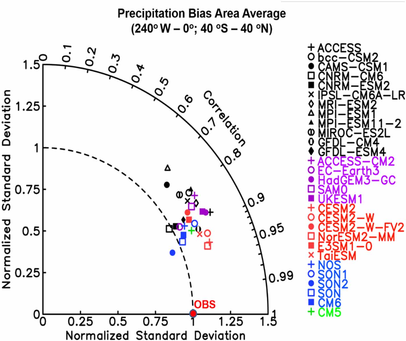
Table 1 and figure 1 show rspatial and σspatial relative to GPCP for all the models. rspatial values are between 0.69 and 0.94 with the SON group showing higher correlations (0.82–0.94) than the NOS group (0.69–0.90). Normalized σspatial mostly exceed 1, i.e. most models exhibit larger spatial variability than observations (CNRM models are the exception, with σspatial from 0.99 to 1.03). There are similar ranges for σspatial, 0.99–1.27 for NOS and 1.05–1.24 for SON. Table 1 also reports mean (spatially-averaged) biases whose magnitudes are generally smaller for NOS (0.17–0.68 mm d−1) than SON (0.34–0.78 mm d−1). The mean absolute bias, a measure of the magnitude of biases, are higher for NOS (0.80–1.34 mm d−1) than SON (0.65–1.11 mm d−1). The model ranking of the mean absolute biases can be found in figure 2, which shows that the best performers belong to several SON2 models.

Figure 1. Taylor diagram showing the normalized standard deviation of oceanic (40°N–40°S) surface precipitation (PR: mm d−1) and correlation with GPCP for each model (see the legend listed on the right). Not shown is the centered root-mean-square error, which is the distance from any point to the reference point (red dot), labeled 'OBS', on the horizontal axis. Different colors represent models without falling ice radiative effects (FIREs) (black), with FIREs using GA71 scheme (purple), with FIREs using MG1 or MG2 (red), and multi-model means (MMMs) for different groups and subgroups of CMIP6 and CMIP6 (CM6) MMM (blue) and CMIP5 (CM5) MMM (green). See SI table S1 for the model acronyms and CMIP6 model groups and subgroups.
Download figure:
Standard image High-resolution image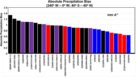
Figure 2. The ranking of mean absolute bias of surface precipitation (PR: mm d−1) against GPCP for each CMIP6 model (1)–(23), with NOS group members in black colored bars, SON1 subgroup members in purple colored bars, and SON2 subgroup members in red colored bars, and CMIP6 group (24, 27), subgroup (25, 26), CMIP6 (28) and CMIP5 (29) MMMs in blue colored bars. The reference data is GPCP for ocean-only latitude belts of 40°N–40°S. The annual time average is over 1980–2014 except CMIP5 for 1980–2005. See SI table S1 for the model acronyms, groups and subgroups.
Download figure:
Standard image High-resolution imageComparing models in the SON1 (purple) and SON2 (red) subgroups (table 1 and figure 1), all five SON1 models have lower correlations (0.82–0.87) than four of the SON2 models (full range 0.84–0.94, although four models are 0.91 or above). The SON1 mean bias range (0.44–0.78 mm d−1) is shifted higher than SON2's (0.34–0.70 mm d−1), and SON1 also has generally higher mean absolute biases (0.89–1.11 mm d−1) than SON2 (0.65–1.00 mm d−1). SON1 spans a wider range of normalized σspatial (1.05–1.24 for SON1 and 1.13–1.20 for SON2), implying that the shift down in mean absolute bias is largely explained by the improved rspatial, i.e. due to better matching the shape of precipitation patterns rather than the magnitude. In terms of the patterns of precipitation in our studied ocean regions, the SON1 models therefore show worse performance than the SON2 models, and in general are comparable to the NOS models (figure 1). While it is encouraging to see the higher correlations, smaller mean biases and smaller mean absolute biases in SON2 than in SON1, one must keep in mind that all of SON2 models still exhibit considerably larger σspatial than observations.
Averaging over multiple models usually results in better performance (Gleckler et al 2008). For example, σspatial for SON2 is reduced to 0.94 while its component models span 1.12–1.20; and SON2 has the highest correlation and the lowest absolute bias among the groups (figure 1). SON is the best performing group in terms of correlation and σspatial but not RMSB (figure 1), resulting from averaging of the SON1 (low correlation and high spatial variability) and SON2 (high correlation and low spatial variability) subgroups, which contributes to slightly improved performance for CM6 compared to that of CM5 (also table 1) in terms of σspatial (1.05 vs 1.1), mean bias (0.51 vs 0.54 mm d−1) and mean absolute bias (0.78 vs 0.85 mm d−1).
The geographical patterns of annual mean precipitation biases for each model are shown in SI (figure S1). The three best performing models are the SON2 models NorESM2-MM, CESM2 and CESM2-WACCM. While the models within the NOS group are relatively poorer in terms of our metrics, we found that the CMIP6 multi-model mean (CM6) shows reduced bias compared to CMIP5 (CM5), and that the inclusion of more models in the SON2 group with its MG2 cloud scheme contributes to this improved performance.
3.2. Spatial patterns of annual mean precipitation biases for different groups of models
In this section, we compare the spatial patterns of (1) biases for NOS, SON, SON1, SON2, CM6 and CM5 groups against GPCP observations, (2) differences between some groups and (3) changes in the absolute biases from one group to another for the annual-mean climatology. The latter is defined as abs (NOS—GPCP) minus abs (SON—GPCP) in each grid cell, for example. The mapped positive changes in the absolute biases proceeding, for example, from the first group (NOS) to the second group (SON), signify improved performance of the second group (SON) relative to that of the first group (NOS) against GPCP. Pooled t-tests (Bhattacharyya 2013) are used to identify regions with significant differences (at the 95% level) between groups, accounting for the difference in group size. These regions are hatched in figures 3(e)–(h). A number of questions can be addressed. For example, is there any improvement in spatial patterns and biases from CMIP5 to CMIP6? Does the difference in the spatial pattern of precipitation biases correspond to different treatments of ice-cloud radiative properties in the two SON subgroups?
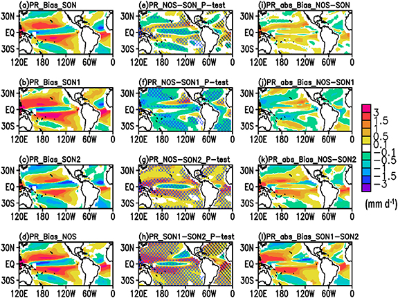
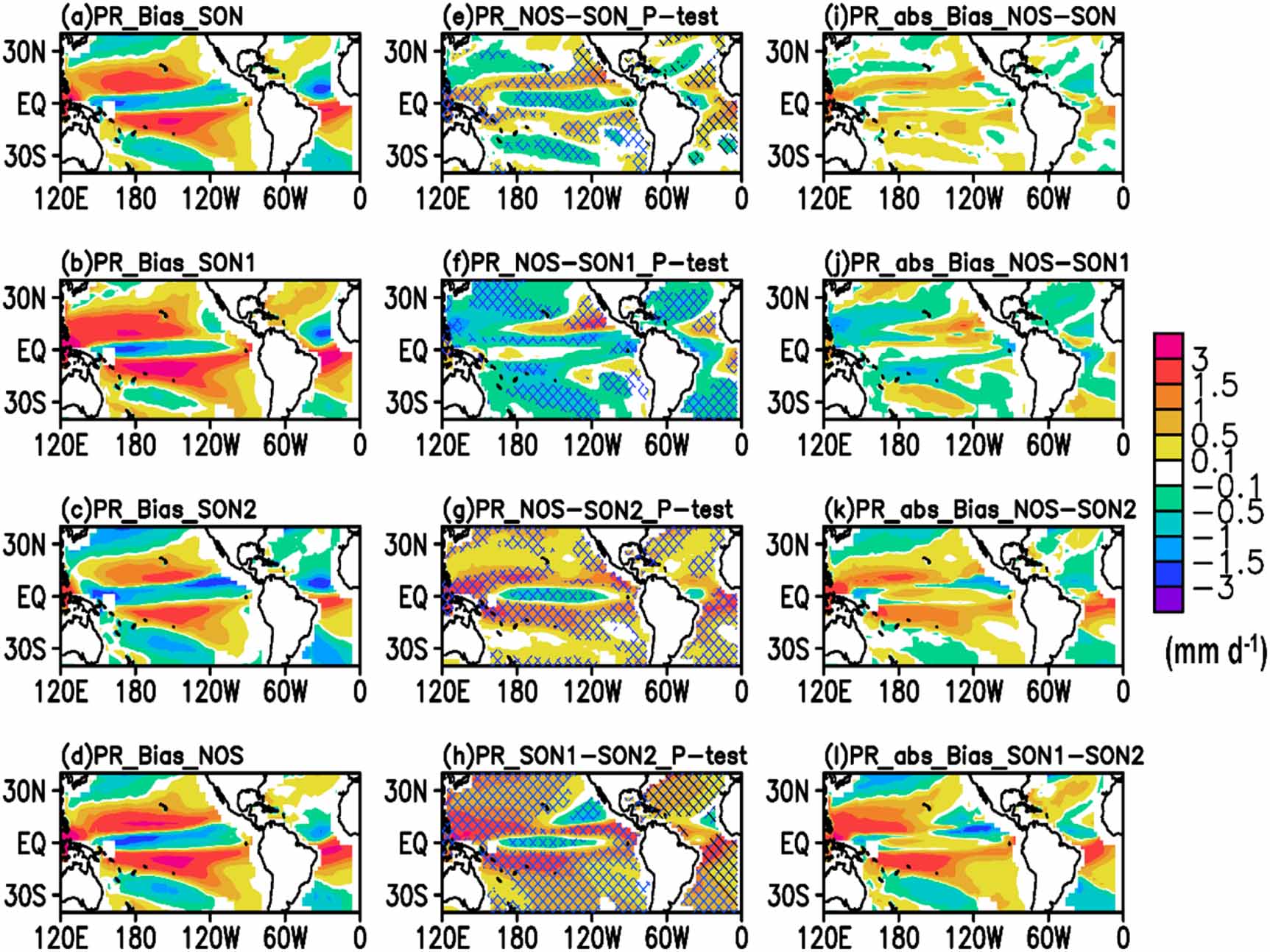
Figure 3. Left column shows annual mean bias of ocean-only surface precipitation (PR: mm d−1) against GPCP for (a) group of CMIP6 models with falling ice radiative effects (SON), (b) subgroup SON1 (GA71 cloud scheme, see text), (c) subgroup SON2 (MG2 cloud scheme), and (d) group of models without falling ice radiative effects (NOS). Middle column shows the difference (e) between NOS and SON (NOS—SON), (f) between NOS and SON1 (NOS—SON1), (g) between NOS and SON2 (NOS—SON2) and (h) between SON1 and SON2 (SON1—SON2) with stippled areas that show 95% significance level with pooled t-tests. Right column (i)–(l) is the same as middle column (e)–(h) except for the absolute bias difference, with positive values indicating improvement. The annual time average is over 1980–2014.
Download figure:
Standard image High-resolution imageFigures 3(a), (b), (c) and (d) show the precipitation biases relative to GPCP for SON, SON1, SON2 and NOS, respectively. Over the convective zones (ITCZ, SPCZ and Tropical Warm Pool) all the groups underestimate precipitation, but overestimate it over the trade wind regions. Over the latter regions, in general, biases are the smallest in SON2 (less than 1.6 mm d–1) with a slight mitigation of the double ITCZ (figure 3(c)). Otherwise, the spatial patterns of biases for SON, SON1 and NOS (figures 3(a), (b) and (d)) are similar in structure, albeit with different magnitudes.
Both NOS—SON2 and SON1—SON2 differences (figures 3(g) and (h)) are generally positive except along the equator and, for SON1—SON2, for areas west of the coast between approximately Mauritania and Sierra Leone in Africa. This means that the double ITCZ is significantly reduced in SON2 relative to either NOS or SON1. A possible explanation is that indirect changes in circulation from NOS to SON2 could affect the simulations of trade wind via radiation–circulation coupling (Li et al 2014a, 2020). This mechanism can result in substantial improvements for SON2 over NOS as seen from the patterns of changes in absolute biases from NOS to SON2 (figure 3(k)) except for the eastern Pacific ITCZ as noted in Li et al (2020). There is less improvement from NOS to SON (figures 3(e) and (i)), due to cancellation in biases in parts of the study domain between SON1 and SON2 (figures 3(f), (g), (j) and 3(k)). The deterioration of SON1 relative to SON2 will be discussed in section 4.
Next, we study changes in spatial patterns and biases from CMIP5 to CMIP6 shown in figure 4. For this, we choose CM5 as the reference and present the differences (left column) and the changes in absolute bias (right column) for NOS (figures 4(a) and (f)), SON (4(b) and (g)), SON1 (4(c) and (h)), SON2 (4(d) and (i)) and CM6 (4(e) and (j)) from CM5, respectively, using model output over 1980–2005 for all groups. Once again, hatching denotes regions where differences are significant at p <0.05 according to pooled t-tests. As discussed earlier, the spatially-averaged, mean bias and mean absolute bias over the study domain are reduced from 0.54 to 0.51 mm d−1 and from 0.85 to 0.78 mm d−1 from CM5 to CM6, respectively (see table 1). The changes in spatial patterns from CM5 to CM6 (figures 4(e) and (j)) resemble those between CM5 and SON (figures 4(b) and (g)) over the Pacific and south Atlantic trade wind regions, albeit with slightly smaller amplitudes. It appears that the improvement from CM5 to CM6 is contributed mostly by the SON models (figures 4(b) and (g)) and particularly by the SON2 models (figures 4(d) and (i)).

Figure 4. Left column shows the difference of annual mean ocean-only surface precipitation (PR: mm d−1) between the CMIP5 multi-model mean (MMM) (CM5) and (a) group of CMIP6 models without falling ice radiative effects (NOS), (b) group of CMIP6 models with falling ice radiative effects (SON), (c) subgroup SON1 (GA71 cloud scheme, see main text), (d) subgroup SON2 (MG2 cloud scheme) and (e) CMIP6 MMM (CM6) with stippled areas that show 95% confidence level with pooled t-tests. Right column (f)–(j) is the same as left column (a)–(e) except for the absolute bias difference, with positive values indicating improvement. The annual time average is over 1980–2005 for both CMIP5 and CMIP6.
Download figure:
Standard image High-resolution imageAll CM6 subgroups show reduced biases around the northward edge of the equator. Elsewhere, bias changes occur with opposite sign in different groups: SON1 and NOS both show increased biases near the Maritime Continent and in the north Pacific, offsetting the improvements in SON2. In other parts of the study domain, particularly the south Pacific and throughout the Atlantic, SON1 has degraded performance even relative to NOS, whereas SON2 once again shows greater bias magnitude reductions.
3.3. Seasonal cycle of precipitation bias and mitigation of double ITCZ
The seasonal cycles of the double ITCZ index from each model and model groups are shown for the Pacific Ocean (figures 5(a) and (b)) and Atlantic Ocean (figures 5(c) and (d)). The double ITCZ index is defined as the precipitation bias averaged over the area of (150°W–100°W, 30°S–EQ) for the Pacific Ocean and over the area of (35°W–0°, 20°S–EQ) for the Atlantic Ocean, respectively, following Bellucci et al (2010) and Hirota et al (2011). These regions are selected as a double-ITCZ metric because the observed ITCZ is located north of the equator except for a brief period in March and April (e.g. Zhang 2001, Haffke et al 2016), and excess heavy precipitation south of the equator is a consequence of models generating an unrealistic double ITCZ.

Figure 5. (a) Pacific double ITCZ index defined as the precipitation bias averaged over (150°W–100°W, 30°S–EQ) against GPCP observation for groups of models (NOS, SON, SON1, SON2, CMIP5 and CMIP6). (b) Same as (a) but for each CMIP6 model (table 1). (c) Same as (a) but for Atlantic double ITCZ index which is defined as the precipitation bias averaged over (35°W–0°, 20°S–EQ) against GPCP observation. (d) Same as (c) but for each CMIP6 model.
Download figure:
Standard image High-resolution image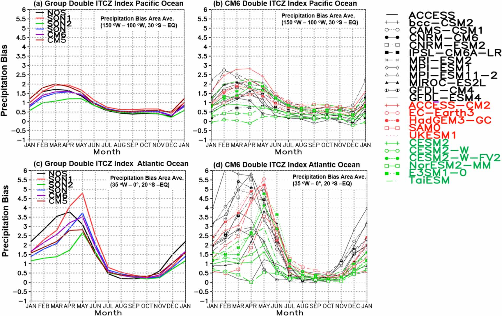
Figure 5 shows that the amplitude of the annual mean bias is largely determined by the biases over November to June for all models and model groups although there is a small bias of approximately 0.5 mm d–1 from July to November. Figures 5(a) and (c) show that, all other model groups exhibit a stronger double-ITCZ bias relative to GPCP than SON2 does, ranging from 1.2 to 2 mm d–1 for the Pacific Ocean in February–May (figure 5(a)) and from 2.8 to 4.7 mm d–1 for the Atlantic Ocean (figure 5(c)) in April and May. By contrast, the SON2 biases peak at ~1.1 mm d–1 in the Pacific and 2.7 mm d−1 in the Atlantic. In terms of the index peak, it is suggested that SON1 performs poorly over both regions while SON2 is the best performer. A degradation in performance from CM5 to CM6 occurs in the Atlantic, driven primarily by NOS prior to March and by SON1 from April–June. SON2 is the only case showing consistent improvement.
For individual models, CESM2-WACCM has the smallest index in the boreal spring (0.25 mm d–1) over the Pacific (figure 5(b)) and 0.5 mm d–1 over the Atlantic (figure 5(d)), followed by NorESM2-MM, CESM2 and TaiESM. The two other SON2 models (E3SM-1-0 and CESM2-WACCM-FV2) have values as large as those in NOS and SON1 models over the Pacific (figure 5(b)). The other models show a wide range of biases in spring and early summer over both oceans. Over the Atlantic, the SON2 models generally outperform the other groups in spring but their later peak in May and June results in no performance improvements then.
4. Discussion and conclusions
Previous work using controlled simulations in a single GCM has shown that FIREs can drive changes in circulation and precipitation. While most GCMs participating in the earlier phases of CMIP5 do not consider FIREs, in the latest CMIP6, more GCMs (11 out of 23) include FIREs. In this study, we have quantified the differences in simulated precipitation between subsets of models without FIREs (NOS) and with FIREs (SON). We have also discussed the progress from CMIP5 to CMIP6, focusing on the tropical and subtropical Pacific and Atlantic oceans between the latitudinal belts of 40°S and 40°N against GPCP observations.
The CMIP6 multi-model mean (CM6) has reduced biases relative to GPCP observations compared with the CMIP5 multi-model mean (CM5), and the group of models including FIREs (SON) contributes the most to this reduced bias. As shown in table 1, the mean biases are 0.59, 0.51 and 0.54 mm d–1 while the mean absolute biases are 0.71, 0.78 and 0.85 mm d–1 for SON, CM6 and CM5, respectively. The group of models without FIREs (NOS) shows larger bias (0.44 mm d–1 for the mean bias and 0.86 mm d–1 for the mean absolute bias). Within SON, there are two main schemes that have been implemented for the treatment of atmospheric falling ice and we further split the SON subset to investigate this. In subgroup SON1, the falling ice mass is included in the radiative transfer, but a single ice particle distribution is used. In SON2, the cloud ice and falling ice are handled separately, with different particle distributions. Subgroup SON2 mitigates precipitation bias drastically, including the double ITCZ bias, while subgroup SON1 does not, as seen from their mean biases (0.50 vs 0.68 mm d–1), mean absolute bias (0.65 vs 0.94 mm d–1), observation-normalized σspatial (0.93 vs 1.15) and rspatial (0.92 vs 0.88) compared with observations.
For individual CMIP6 models, the four best performance models in terms of the mean absolute bias are in SON2 and ranked in order of ascending bias, they are NorESM2-MM, CESM2, CESM2-WACCM and TaiESM1 (figure 2 and table 1), while the three worst performance models are in NOS group (MPI-ESM1-2, CAM5-CSM1 and NorCPM1). Four of five SON1 models are in the best ten in terms of lowest mean absolute bias, although EC-Earth3-Veg is among the five highest bias ranking. SON shows improved performance relative to NOS according to our metrics, and this is driven by SON2, and the SON models drive the improved performance of CM6 relative to CM5. These differences among the model groups also appear in the spatial pattern of precipitation biases and seasonal cycles of double ITCZ indices over the Pacific and Atlantic Ocean.
The substantially different performance between SON1 and SON2 subgroups merits further investigation, in particular, SON2 produces a remarkable reduction of annual and seasonal mean precipitation biases, including the mitigation of the double ITCZ problem over the Pacific and Atlantic Oceans. As mentioned in section 2, SON2 models use separate cloud ice and falling ice contents with different effective ice diameters to calculate ice-cloud radiative properties, while SON1 models uses combined frozen water content (falling ice + cloud ice) with a single effective ice diameter to calculate ice-cloud radiative properties. It is well known that ice hydrometeor radiative properties vary vertically and are different between cloud ice and falling ice, due to their diverse crystal habits and growth processes (Heymsfield et al 2002, Heymsfield 2003). How representative are the ice-cloud radiative properties formulated using a single effective radius size, shape and number of concentrations as in SON1? To answer this question, an in-depth study of ice-cloud radiative properties in individual models, in particular in SON1 models, is needed.
The radiation–circulation coupling mechanism has previously been used to explain some of the differences in precipitation between NOS and SON models (Li et al 2014a, 2016, 2020). This mechanism can be supported by how atmospheric falling ice reduces outgoing longwave radiation at the top of atmosphere (TOA), and changes the vertical heating rate in such a way that the columns in convective areas are stabilized. Li et al (2020) found that CMIP6 SON-NOS multi-model mean differences in TOA longwave fluxes generally follow the patterns expected due to the inclusion of FIREs, implying that changes in other processes between the models do not counteract the effect of FIREs. The exclusion of FIREs invigorates convection, resulting in stronger downdrafts and enhanced low-level outflow from convective zones (ITCZ, SPCZ and Tropical warm pool) into the trade wind regions, weakening the easterly trades in NOS models and inducing meridional divergence anomalies. The weaker surface wind stress in the trade wind regions results in apparent advection of low-level moist and warm air over the trade wind regions (see SI figure S2) and high biased surface precipitation rates. The biases of surface winds, SSTs and precipitation are mitigated over most of the Pacific and Atlantic trade wind regions in SON models.
For the significant differences in simulated precipitation between SON1 and SON2, our preliminary analysis shows that there are differences in circulation over the trade wind regions (not shown). This requires an in-depth investigation which is forthcoming but beyond the scope of this analysis.
SON2 models show a substantial improvement in mitigating the double ITCZ bias, which was also reported in Woelfle et al (2019) for a single model. Using CESM2-CAM6 with MG2 cloud microphysics, they found significant improvements in southeast Pacific shortwave cloud forcing (related to low clouds), sea surface temperature and ITCZ climatology, including mitigation of the double ITCZ, compared to CESM1-CAM5.
This study concludes that we have found evidence within CMIP6 models that FIREs have non-negligible impacts relative to typical model biases in current state-of-the-art GCMs. In particular, this evidence is consistent with improved simulation of oceanic precipitation patterns when models allow cloud ice and falling ice mass to interact with radiation. It is encouraging to see more GCMs in CMIP6 include FIREs, although we cannot attribute the improvement to FIREs exclusively. We can conclude that models using the MG2 cloud scheme show greatly improved mean spatial statistics of oceanic precipitation, but these models may have other commonalities that contribute to the improved performance. Such commonalities cannot be distinguished in our analysis so we acknowledge that while the treatment of this particular physical process may help climate simulation of precipitation, controlled investigation of individual models and further improvement in the treatment of cloud ice–radiation interactions is needed.
Acknowledgments
The contributions by JLL to this study were carried out on behalf of the Jet Propulsion Laboratory, California Institute of Technology, with the National Aeronautics and Space Administration (NASA). We thanks to Dr. Bin Guan from UCLA for his useful analysis tools. The GPCP Version 2.3 Combined monthly Precipitation Data Set, ranging from January 1979 through May 2019, is used [https://psl.noaa.gov/data/gridded/data.gpcp.html.]. The QuikSCAT annual cycle climatology of sea-surface wind speed and direction under all weather and cloud conditions over Earth's oceans is produced from August 1999 to October 2009 (http://podaac-www.jpl.nasa.gov/) for the obs4MIPS project. The monthly mean data are downloaded from APDRC of the IPRC, http://apdrc.soest.hawaii.edu/datadoc/qscat_mwf.php.
Data availability statement
No new data were created or analysed in this study.