


Abstract
This article analyses the greenhouse gas (GHG) impact potential of improved management practices and technologies for smallholder agriculture promoted under a global food security development program. Under 'business-as-usual' development, global studies on the future of agriculture to 2050 project considerable increases in total food production and cultivated area. Conventional cropland intensification and conversion of natural vegetation typically result in increased GHG emissions and loss of carbon stocks. There is a strong need to understand the potential greenhouse gas impacts of agricultural development programs intended to achieve large-scale change, and to identify pathways of smallholder agricultural development that can achieve food security and agricultural production growth without drastic increases in GHG emissions.
In an analysis of 134 crop and livestock production systems in 15 countries with reported impacts on 4.8 million ha, improved management practices and technologies by smallholder farmers significantly reduce GHG emission intensity of agricultural production, increase yields and reduce post-harvest losses, while either decreasing or only moderately increasing net GHG emissions per area. Investments in both production and post-harvest stages meaningfully reduced GHG emission intensity, contributing to low emission development. We present average impacts on net GHG emissions per hectare and GHG emission intensity, while not providing detailed statistics of GHG impacts at scale that are associated to additional uncertainties. While reported improvements in smallholder systems effectively reduce future GHG emissions compared to business-as-usual development, these contributions are insufficient to significantly reduce net GHG emission in agriculture beyond current levels, particularly if future agricultural production grows at projected rates.
Export citation and abstract BibTeX RIS

Original content from this work may be used under the terms of the Creative Commons Attribution 3.0 licence.
Any further distribution of this work must maintain attribution to the author(s) and the title of the work, journal citation and DOI.
1. Introduction
Achieving food security in synergy with preserving natural resources and providing environmental services such as climate change mitigation is a key challenge for sustainable development, and current trends underscore the need for new development trajectories (UNGA 2015, FAO 2011, 2012, 2016, Campbell et al 2014, Lal et al 2015). Under a 'business-as-usual' (BAU) scenario, global agricultural production may increase by 60% by 2050, predominately in developing countries, with net arable land area increasing by 70 million ha (Alexandratos and Bruinsma 2012). Conventional cropland intensification and conversion of natural vegetation to agriculture typically increase N2O and CH4 emissions and reduce carbon stocks in soils and biomass (FAO 2014, Smith et al 2014). Currently, agriculture contributes 5.0–5.8 Gt CO2e, or 10%–12%, annually of global anthropogenic GHG emissions (Smith et al 2014). Using the BAU projection by Alexandratos and Bruinsma (2012), FAO (2014) estimates that global GHG emissions from agriculture would increase by 18% (2030) and 30% (2050) compared to 2001–2010, excluding forestry and other land use change. WRI (2013) estimates that by 2050 under BAU development, agricultural and land-use change emissions would constitute 70% of GHG emissions levels targeted to limit global average temperature change to 2 °C in 2100.
Achieving global food security without drastic increases in GHG emissions necessitates policy measures to move from a BAU path and initiate a transformation to low emission development (LED). LED depends upon national, cross-sectoral strategies that foster economic growth and food security while simultaneously reducing GHG emissions compared with BAU scenarios. For example, GHG emissions might increase only logarithmically as a function of production, instead of linearly or exponentially.
National and international policy agendas increasingly recognize the need for LED in the agriculture sector. Under the Paris Agreement within the United Nations Framework Convention on Climate Change, countries committed to develop nationally determined contributions (NDCs) to limit 21st century global temperature to 1.5°-2 °C above pre-industrial levels. The Sustainable Development Goals of the United Nations (UNGA 2015) call to (i) take urgent action to combat climate change and its impacts; (ii) protect, restore, and promote the sustainable use of terrestrial ecosystems; and (iii) ensure sustainable consumption and production patterns. Many governments recognize agriculture as an important sector for addressing GHG emissions: 104 of 162 countries that submitted an intended NDC included agriculture in their targets (Richards et al 2016).
Revising and aligning domestic resources and international finance for agriculture can be a key enabling mechanism for implementing LED. Multilateral financing sources, such as the Green Climate Fund and the Global Environment Facility, provide targeted finance for climate change adaptation and mitigation in agriculture. In 2015, global finance sources contributed US$10.4 billion in official development aid to the agriculture, forestry, and fisheries sectors (OECD 2016). Government expenditure on agriculture remains significant despite declines in developing countries (Fan and Rao 2003, Akroyd and Smith 2007). The African Union's Comprehensive Africa Agriculture Development Programme targets increases in national spending on agriculture to at least 10% of national budgets (AU 2003). Leveraging these resources to address GHG emissions is an opportunity to meet climate commitments while addressing food security.
Several studies have analyzed the technical mitigation potential of selected agricultural options applied in isolation (Smith et al 2007, Wollenberg et al 2016, Gerber et al 2013, IPCC 2006, World Bank 2012, Del Grosso et al 2009). However, agricultural investments are implemented neither in isolation nor solely for climate change mitigation objectives. To understand the potential for agricultural development to mitigate climate change and whether increased production and economic growth can be decoupled from GHG emissions and carbon losses, we estimated GHG emissions from projects designed to improve food security in smallholder agriculture. In the analysis we focus on GHG emissions per hectare and per quantity of production, while we do not present detailed results on the GHG emission impacts at scale, due to the associated uncertainties involved. We synthesize results from 26 diverse smallholder development projects, including 134 crop and livestock production systems spanning 15 countries across Africa (9), Asia (2), and Latin America (4), implemented as part of the US Government's Feed the Future initiative7, funded by the United States Agency for International Development (USAID).
2. Data and methodology
We selected 26 development projects from the Feed the Future initiative and collected data on project targets through semi-structured interviews and a standardized review of project documentation and monitoring data. We analyzed project targets for their estimated GHG impacts using the FAO EX-Ante Carbon Balance Tool (EX-ACT) (Bockel et al 2013, Grewer et al 2013, Bernoux et al 2010). The methodology for sampling, data collection, and GHG impact estimation is summarized below. Further details are available in Grewer et al (2016).
2.1. Selection of projects for analysis
We rated 150 Feed the Future agriculture projects as unlikely, possibly, or likely to have significant effects on net GHG emissions. For projects with likely GHG impacts, we selected 36 ongoing projects based on (i) geographic and project diversity, and (ii) robust monitoring and evaluation reporting by implementing partners to USAID. Implementing partners are generally local or locally-based organizations with long experience in the agricultural sector and deep knowledge about the region. We used a phased approach, beginning with field visits to collect data and subsequent analyses of nine projects in two pilot countries (Bangladesh and Mali). Building on lessons from these pilots and to maximize coverage of this investigation, we conducted a combination of field visits, remote interviews with implementing partners, and content analysis of USAID reporting documentation. After primary data collection, we removed ten projects due to incomplete information or concerns about data quality.
2.2. Data collection and data quality assurance
Data collection comprised four steps:
- 1.Review of project documentation: We extracted quantitative data on project targets by reviewing the binding project design document used in selection for financing by USAID. We collected all available data from project monitoring and update reports that implementing organizations provide on a quarterly basis to USAID, generated by a dedicated project monitoring system.
- 2.Completion of a written questionnaire by project implementing organizations: Each implementing organization completed a detailed questionnaire tailored to specific project focal areas and context conditions. The questionnaires considered a comprehensive range of project impacts related to GHG emissions and carbon sequestration in agriculture, forestry, and land use identified based on IPCC (2006). As a basis for this questionnaire, we used a generic instrument that has been widely used in other contexts to collect data for the EX-ACT tool (supplement 1 available at stacks.iop.org/ERL/13/044003/mmedia).
- 3.Face-to-face or telephone interviews: We conducted interviews with project implementing organizations guided by a semi-structured questionnaire (supplement 2). Based on the analysis of the data procured in (1) and (2), we prepared additional priority questions specific to each project.
- 4.Interview follow-up: We sent targeted, written follow-up questions to implementing organizations to collect quantitative project data that were not available during the interview or for which we sought a second confirmation. We provide one instance of anonymized follow-up questions as an illustration (supplement 3).
Most projects were still active at the time of the interview. Nearly all projects had been operating for more than two years, and roughly half were close to ending. Implementing organizations characterized in detail the type of improved practices and technologies supported, and estimated their outcomes at project completion based on targets established with the donor and on progress measured empirically to date. Estimates of targeted area and livestock numbers refer to the total scale of adoption of improved management practices and technologies in farmers' fields due to project support. Project measures were not focused on implementing improved management on directly controlled pilot areas, but involved scaling mechanisms such as farmers' capacity development and support to mechanization providers and other value chain agents. Implementing organizations' project monitoring systems most commonly consisted of non-representative interviews with project beneficiaries by district-level project staff, and subsequent data aggregation across districts.
Data about project impacts on crop yield and post-harvest loss reduction are particularly important for this study. Project implementing organizations indicated high confidence in estimates of crop yield changes, based on beneficiary interviews. Measured yield improvements on pilot and experimental plots provided further reference points. When reported yield increases in farmers' fields exceeded the performance on pilot plots, we considered reported increases unreasonable and withdrew them from this analysis.
Data quality of post-harvest loss reduction varied among projects. Projects with a central focus on post-harvest loss reduction—particularly in the dairy, rice, and vegetable value chains—had detailed post-harvest loss surveys with high data quality from processing and marketing agents. Projects with marginal components on improved milling and/or storage—mainly maize and other crops—relied on interviews with beneficiary farmers. While we employed data quality assurance measures (see below), data quality of post-harvest loss estimates from beneficiary farmers was estimated to be low by implementing organizations.
Regarding the scale of implementation, data quality may suffer from non-representative sampling of beneficiaries, and poor execution of interviews by the implementing organization or its sub-contractors. Representative household data on project beneficiaries collected by independent third-party stakeholders are commonly unavailable when analyzing agricultural investment projects across countries and larger scales.
In order to ensure data in this study were of sufficiently high quality to draw robust conclusions, we employed the following data quality management measures:
- Data flagged by project implementing organizations as subject to major uncertainty and project targets unaccompanied by a reasonable amount of monitoring data to substantiate claims were withdrawn from the analysis.
- We only included direct GHG impacts; we excluded data on indirect GHG co-benefits for which no good data documentation was available.
- We focus primarily on GHG impacts per hectare and GHG emission intensity, as these measures are a function of practices supported by projects, not by the scale of adoption. There is a very high level of certainty that the data collection process accurately characterized the promoted management practices.
- We interpret extent of adoption mainly to interpret scalability and barriers to adoption of improved practices and technologies. We do not present the gross GHG estimates at scale in a detailed manner as they introduce more uncertainty.
2.3. Temporal and geographic boundary setting and leakage
Increases in forest biomass or soil carbon that occur in response to changes in land management continue only until these carbon pools reach a new equilibrium. We estimated the influence of new agricultural practices on average annual GHG emissions over 20 years following project initiation, consistent with time frames commonly considered for carbon stocks to reach equilibrium (IPCC 2006). This approach assumes that growers continue to use agricultural practices introduced by development projects over this 20 year period, long after development assistance ends. If growers or land managers immediately abandoned the supported production practices, e.g. by cutting planted agroforestry trees or discontinuing use of improved livestock feed, the presented GHG benefits would not accrue, and GHG balances would gradually return to the estimates for conventional production systems.
We estimated GHG impacts within the area targeted directly by project actions. When applicable, the studies differentiate between projects' target zones of implementation and the non-target zones that exhibited clear spillover from the project (Bockel et al 2013).
Ultimately, the influence of land management initiatives on national-scale GHG balances needs to consider geographies beyond the project boundaries. Although that complex analysis is beyond the scope of this investigation, correct interpretation of our results requires considering the relationship of project-level to national-level GHG emissions. Projects can influence land use beyond the target area in two ways. First, a project may cause activities that produce GHG emissions to cease or decline locally, but these activities may then appear or increase in another area, usually because the overall demand driving the activity has not changed (leakage). For instance, if a project provides incentives to reduce deforestation on a limited geographical scale while overall strong demand for timber products continues to prevail, deforestation might shift from the project area to another location. Second, if the adoption of improved practices increases income generated per hectare, the project provides incentive to clear natural vegetation for agriculture, assuming sufficient labour and financial resources are available. These dynamics are difficult to estimate as part of ex-ante analyses because doing so requires clear causal pathways that depend strongly on context, as well as quantitative estimates of their strength. Interviews with project implementing partners led us to conclude that these projects were unlikely to have strong influences outside of the target geographies.
2.4. Estimating impacts on GHG budgets
Expected or monitored project outcomes served as input data to EX-ACT to estimate (i) the total GHG impact of agricultural production systems by area, (ii) the GHG impact of individual agricultural practices as compared with BAU practices, and (iii) the GHG emission intensity of production systems prior to and after project implementation.
EX-ACT is an appraisal system developed by FAO that estimates the impact of field activities in agriculture, forestry, and land use on GHG emissions and carbon sequestration as compared with a BAU scenario. The tool accounts for (i) changes in five carbon pools (above-ground biomass, below-ground biomass, dead wood, litter, and soil organic carbon) and (ii) emissions of CH4, N2O, and selected further CO2 emissions (Bernoux et al 2010, Grewer et al 2016). EX-ACT follows the IPCC Guidelines for National Greenhouse Gas Inventories (IPCC 2006) for accounting and generating Tier 1 GHG emission coefficients and carbon stock change factors. For specific mitigation options not covered in IPCC (2006), the tool uses data from the Fourth Assessment Report of the IPCC (Smith et al 2007)8. The IPCC (2006) methodology allows combined use of Tier 1 and Tier 2 data. We used country- and project-specific Tier 2 factors wherever available, otherwise relying on default Tier 1 factors. Furthermore, required coefficients from published reviews (Lal 2004) or international databases (USDE 2007) were used where appropriate. To calculate the GHG impact of each project, the analysis accounted for GHG emissions and carbon sequestration resulting from the following processes:
- Changes in carbon stocks from above- and below-ground biomass: Default values for above- and below-ground biomass stocks, biomass growth rates, and biomass carbon content for various climates and land uses correspond to Tier 1 estimates from IPCC (2006). We estimated biomass of agroforestry systems on an ad-hoc basis using species-specific biomass stocks and growth rates from the literature (Somarriba et al 2013, Negash et al 2013, Zuidema et al 2005, Fuwape and Akindele 1997), as well as information on tree-stand densities provided by project implementing organizations.
- Changes in carbon stocks from litter and dead wood: We assumed no litter and dead wood pools in all non-forest categories. For land use change between forest and non-forest categories, we used default carbon stock values from IPCC (2006).
- Changes in soil carbon stocks: We estimated soil organic carbon stocks for mineral soils to a depth of 30 cm using default values from IPCC (2006). When soil organic carbon changes occurred over time (due to land use change or management change), we assumed a default period of 20 years to reach a new equilibrium soil carbon stock. Improved management practices on cultivated cropland were analyzed using carbon change rates (Smith et al 2007) instead of a carbon stock difference approach.
- Emissions of CH4, N2O, and selected further CO2 sources: We estimated CH4 emissions from flooded rice systems using IPCC (2006) and project-specific information on rice crop management. CH4 and N2O emissions from biomass burning were estimated using IPCC (2006); crop residue biomass quantities were estimated based on project-specific crop yields. We estimated direct N2O emissions from field application of nitrogen using the IPCC's default GHG emission factors for flooded and non-flooded conditions (IPCC 2006). We calculated nitrogen application rates based on project-specific data for synthetic and organic fertilizer application rates. Direct measurements published by Gahire et al (2015) informed a preliminary emission factor for fertilizer deep placement in irrigated rice systems. Further CO2 emissions due to fertilizer and pesticide production, transport, and storage, as well as from agricultural infrastructure establishment, were estimated using GHG emission factors from Lal (2004). We estimated GHG emissions from electricity production using coefficients from the International Energy Agency (USDE 2007), and GHG emissions from the consumption of fuels for farm operations using IPCC coefficients (IPCC 2006).We estimated CH4 emissions from enteric fermentation using a partial Tier 2 approach, considering project-specific animal weight, IPCC guidelines for cattle and sheep (IPCC 2006), and guidelines from Dittmann et al (2014) for camels. For N2O and CH4 emissions from manure management, we used the Tier 2 method from IPCC (2006), considering project-specific data on animal weight where available. We used methods described in Smith et al (2007) to estimate the influence of improved feeding practices, application of dietary additives, or improved breeding practices on livestock-related GHG emissions.
We converted all GHG impacts to CO2 equivalents assuming a global warming potential of 34 for CH4 and 298 for N2O (Myhre et al 2013). We define the term GHG impact as the net effect of all GHG emissions and carbon sequestration that occur due to a production system or practice. Throughout this analysis negative numbers denote GHG emission reductions and carbon sequestration, and positive numbers indicate GHG emissions unless the direction of change is otherwise indicated in the text.
We estimated GHG emission intensity as GHG emissions per (i) ton (t) of annual crop product, (ii) ton of live animal weight at slaughtering, or (iii) 1000 liters (l) of milk. For crops and dairy, product quantities are considered after subtracting post-harvest losses. GHG impacts on soil and biomass carbon stocks were included when estimating GHG intensities. EX-ACT is intended for use in data-scarce contexts, where detailed data on soils, crop physiology, weather, and field measurements of GHG emissions and carbon stock changes are not available. The tool indicates the magnitude of GHG impacts. The method we used does not provide plot or season-specific estimates of GHG emissions, and is not suited to ground-truth actual, realized GHG impacts.
3. Results
Results come from 26 Feed the Future projects that reported direct impacts on 4.8 million ha of cropland, and included 32 crop types, four types of livestock, and 19 improved agricultural management practices or technologies. The dataset includes 132 different production systems. Supplement 4.1 and 4.2 identify frequency and scale of (i) analyzed crop types and (ii) improved agricultural management practices or technologies.
The displayed results identify the ordinary arithmetic mean of GHG impacts across all occurrences of production systems or practices. Thus, each occurrence of a production system/practice is given the same importance for the summary results, independent from the projected geographic scale of its adoption within the specific analyzed project contexts.
3.1. GHG impacts by production system
Prior to project implementation, the 32 crop products analyzed exhibited average annual GHG impacts of 0.11–1.26 tCO2e ha−1 (lower and upper quartile boundaries). The production systems analyzed had low GHG impacts per hectare, typical for low-input systems as compared with mechanized agriculture (Johnson et al 2016, Camargo et al 2013). In the long term, if low-input systems degrade soils, they may lead to losses of soil carbon and more frequent clearing of natural vegetation, which result in additional losses of carbon stocks.
Table 1. Annual GHG impacts per hectare by main production systems.
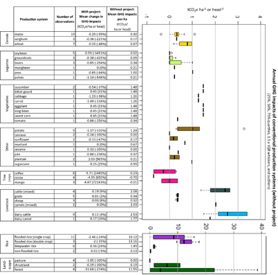 |
Table 1 shows the average annual GHG impacts of conventional production systems prior to project interventions, and the average change in GHG impacts resulting from project implementation. The boxplots identify the lower quartiles, median and upper quartiles of the GHG impacts of each conventional production system prior to project intervention9. These estimates are per hectare or per head of livestock; estimates per unit of product appear in the following sections. While table 1 displays results for each production system, we below identify results across aggregated crop categories wherever this aides interpretation.
When comparing GHG impacts of cropping systems before project implementation, the highest annual net GHG emissions per hectare came from: irrigated rice (10.12 tCO2e ha−1 and 13.16 tCO2e ha−1 for single and double cropped rice respectively), selected vegetable crops (e.g. cucumber, bitter gourd, eggplant, long bean, and sweet corn: 1.48 tCO2e ha−1, cabbage and carrot: 1.26 tCO2e ha−1), and potato (1.24 tCO2e ha−1). Conversely, GHG impacts from cocoa (−0.7 tCO2e ha−1) and coffee (−0.23 tCO2e ha−1) were negative, meaning overall carbon sequestration (e.g. in soil and biomass) exceeded GHG emissions (e.g. from fertilizer use). Livestock production systems also contributed to GHG emissions in the projects. Dairy cattle (2.53 tCO2e head−1), mixed cattle (2.08 tCO2e head−1), and mixed camels (2.03 tCO2e head−1) had the greatest annual GHG emissions per head. Goats (0.34 tCO2e head−1) and sheep (0.33 tCO2e head−1) produced lower annual GHG emissions.
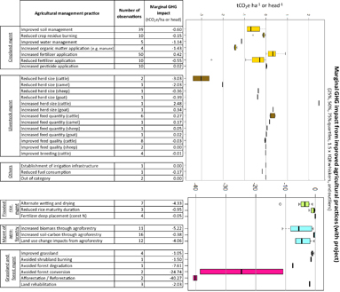
Table 2. Annual GHG impacts per hectare from changes in agricultural practices.
 |
GHG impact per hectare decreased in most production systems due to project implementation. The 32 crop products analyzed exhibited average annual GHG impacts of −0.52 to 0.43 tCO2e ha−1 (lower and upper quartile boundaries). The largest changes were observed for irrigated rice, where GHG emissions declined on average 2.15 tCO2e ha−1 per rice crop. Project interventions across agroforestry systems10 increased annual net carbon sequestration on average by 6.14 tCO2e ha−1. Other cereals, legumes, and vegetable crops were characterized mainly by small annual changes (−0.78 tCO2e ha−1, −0.56 tCO2e ha−1, and −0.49 tCO2e ha−1, respectively), mostly due to soil carbon sequestration. Interventions in livestock production systems moderately increased annual GHG emissions per head, mainly due to increased feed intake. Mixed cattle (0.19 tCO2e head−1), dairy camels (0.17 tCO2e head−1), and dairy cattle (0.11 tCO2e head−1) experienced moderate increases in GHG emissions; estimated changes for goats and sheep were negligible.
3.2. GHG impacts by type of improved agricultural practice
Table 2 shows the average annual GHG impacts resulting from changes in agricultural practices per hectare or livestock head.
Improved management practices of non-flooded annual cropland led on average to annual net GHG reductions of 0.15 tCO2e ha−1. Annual impacts ranged between GHG emission reductions of 0.60 tCO2e ha−1 and GHG emission increases of 0.22 tCO2e ha−1 (lower and upper quartile boundaries). Main impacts result from increasing soil carbon sequestration driven by organic matter application and improved soil management, as well as changing N2O emissions from adjusted fertilizer application rates. These changes are relatively small compared with those resulting from interventions in flooded rice systems, agroforestry, or land use change, described below.
Alternate wetting and drying reduced annual GHG emissions from between 4.80 and 2.19 tCO2e ha−1 (lower and upper quartile boundaries), whereas shortening of the growing season for rice crops reduced average annual GHG emissions by 0.95 tCO2e ha−1.
The expansion and improvement of agroforestry systems led to large GHG mitigation benefits per hectare compared with annual cropping systems. For example, increases in biomass carbon stocks sequestered on average 5.22 tCO2e ha−1 yr−1 over an estimated 20 yr period. The small areas to which projects introduced various forms of improved forest management likewise provided large GHG benefits per hectare: Avoided forest conversion to non-forest land uses on average prevented annual carbon losses of 24.74 tCO2e ha−1, whereas afforestation generated average annual carbon sinks of 40.27 tCO2e ha−1. Avoided forest degradation (e.g. through increasing forest stand density, managing tree species composition, preventing forest fire, improving forest pest management) generated annual carbon sinks of 7.61 tCO2e ha−1.
Project interventions in livestock production systems made large GHG impacts through reducing or increasing total livestock numbers (cattle: 2.48 tCO2e, goats: 0.34 tCO2e for each head, respectively). Projects supported increasing livestock herds where they identified readily-available market demand, market infrastructure and sustainable production capacity. Reductions in herds were encouraged where projects concluded that current herds could not be managed efficiently with given resources, marketing opportunities were limited, and/or herders could link to more effective forms of financial savings and risk management of household assets.
Increasing feed quantity significantly increased annual GHG emissions from cattle (0.27 tCO2e head−1) and camels (0.17 tCO2e head−1). The conservative methodology used to assess GHG impacts of improved breeding and feed quality (Smith et al 2007) indicates only small benefits from these practices for GHG emissions per head.
3.3. GHG emission intensity of agricultural products
GHG emission intensity is a useful indicator of LED that strives to increase food production while minimizing GHG emissions. GHG emission intensity is determined by (i) GHG impact per hectare of a production system, (ii) crop or livestock product yields, and (iii) post-harvest losses.
Post-harvest losses affect GHG emission intensity but are typically unaccounted for due to data scarcity. The primary management practices promoting post-harvest loss reductions in the projects analyzed were:
- Improved timing of ripening and harvest operations (e.g. avoiding management induced within-field heterogeneity of ripening dates in vegetables; determining harvesting dates based on grain moisture for maize)
- Improved harvesting practices and post-harvest handling (e.g. reducing unnecessary product and plant damages during harvest operations; using of adequately sanitary containers for vegetable transport; ensuring timely transportation and marketing of vegetables and dairy products)
- Improved product processing (e.g. increasing access to small-scale milk processing facilities; improving rice milling facilities)
- Improved product storage (e.g. diffusion of economic and locally adapted storage technologies for grains that reduce losses from fungi, insects and further sources of post-harvest losses)
GHG emission intensity prior to project intervention ranged from −2.50 tCO2e t−1 for cocoa to 38.01 tCO2e t−1 for cattle meat (see table 3). Comparing estimates of GHG emission intensity across product categories can only provide a rough orientation, since any product or calorie quantity (e.g. from cattle meat) cannot be compared to the same quantity from another product category, such as cereals. Instead, comparing the change in GHG emission intensity of single product categories over time provides a clear indication of an improving or worsening situation.
Feed the Future projects reduced GHG emission intensity across nearly all analyzed products, as compared to practices prior to project interventions (table 3) (values for all crops are provided in supplement 4.3). GHG emission intensity declines by an average of −108% across all analyzed products. The strongest net average reductions in GHG emission intensity are achieved for coffee (5.07 tCO2e t−1), cocoa (3.08 tCO2e t−1), and irrigated rice (1.37 and 1.08 tCO2e t−1 for single and double cropped rice, respectively). Projects also reduce the GHG emission intensity of livestock systems. Average GHG emissions per ton of live weight at slaughtering decreases by 10.14 tCO2e t−1 (27%) for cattle, 10.30 tCO2e t−1 (41%) for sheep, and 10.03 tCO2e t−1 (39%) for goats. In dairy systems, projects reduced average GHG emission intensity for cattle milk by 1.73 tCO2e 1000 l−1 (41%) and camel milk by 3.55 tCO2e 1000 l−1 (56%).
Table 3. GHG emission intensity by product.
| Product | Scenario | Total GHG emissions (tCO2e per ha/ head/1000 l milk) | Yield (t per ha/ head/1000 l milk) | Postharvest loss (%) | GHG emission intensity (tCO2e per t/1000 l milk) |
|---|---|---|---|---|---|
| maize | Without project | 0.3 | 2.80 | 0.17 | 0.17 |
| With project | 0.004 | 4.35 | 0.09 | −0.01 | |
| Net difference (%) | −0.3 (−99%) | 1.54 (55%) | −8 ppa (−44%) | −0.18 (−108%) | |
| wheat | Without project | 0.7 | 2.86 | 0.09 | 0.25 |
| With project | 0.3 | 3.34 | 0.03 | 0.11 | |
| Net difference (%) | −0.3 (−48%) | 0.48 (17%) | −6 pp (−61%) | −0.14 (−54%) | |
| soybean | Without project | 0.02 | 0.72 | 0.17 | 0.02 |
| With project | −0.5 | 1.66 | 0.10 | −0.33 | |
| Net difference (%) | −0.6 (−3451%) | 0.94 (131%) | −7 pp (−41%) | −0.35 (−1490%) | |
| groundnuts | Without project | 0.1 | 0.91 | 0.10 | 0.08 |
| With project | −0.3 | 1.05 | 0.05 | −0.20 | |
| Net difference (%) | −0.4 (−425%) | 0.14 (15%) | −5 pp (−52%) | −0.28 (−370%) | |
| sunflower | Without project | 0.2 | 0.99 | 0.03 | 0.10 |
| With project | 0.1 | 1.35 | 0.03 | −0.33 | |
| Net difference (%) | −0.1 (−67%) | 0.36 (37%) | 0 pp (0%) | −0.43 (−450%) | |
| sesame | Without project | 0.0 | 0.31 | 0.10 | 0.00 |
| With project | 0.3 | 0.50 | 0.05 | 0.68 | |
| Net difference (%) | NA | 0.19 (62%) | −5 pp (−50%) | NA | |
| coffee | Without project | −0.2 | 0.96 | 0.16 | −0.40 |
| With project | −5.9 | 1.54 | 0.13 | −5.47 | |
| Net difference (%) | −5.7 (2455%) | 0.58 (60%) | −3 pp (−19%) | −5.07 (−1253%) | |
| cocoa | Without project | −0.7 | 0.55 | 0.19 | −2.50 |
| With project | −4.7 | 0.93 | 0.19 | −5.58 | |
| Net difference (%) | −4 (575%) | 0.38 (68%) | 0 pp (0%) | −3.08 (−123%) | |
| cattle meat | Without project | 2.2 | 0.07 | 0.00 | 38.01 |
| With project | 2.3 | 0.11 | 0.00 | 27.87 | |
| Net difference (%) | 0 (2%) | 0.04 (55%) | 0 pp (0%) | −10.14 (−27%) | |
| goat meat | Without project | 0.4 | 0.01 | 0.02 | 25.53 |
| With project | 0.3 | 0.02 | 0.02 | 15.50 | |
| Net difference (%) | −0.1 (−22%) | 0.01 (63%) | 0 pp (0%) | −10.03 (−39%) | |
| sheep meat | Without project | 0.3 | 0.01 | 0.00 | 25.36 |
| With project | 0.3 | 0.02 | 0.00 | 15.06 | |
| Net difference (%) | 0 (3%) | 0.01 (73%) | 0 pp (0%) | −10.3 (−41%) | |
| cattle milk | Without project | 2.6 | 0.94 | 0.17 | 4.22 |
| With project | 2.6 | 1.74 | 0.08 | 2.49 | |
| Net difference (%) | 0 (0%) | 0.79 (84%) | −9 pp (−57%) | −1.73 (−41%) | |
| flooded rice (single cropping) | Without project | 10.1 | 4.31 | 0.08 | 2.85 |
| With project | 7.7 | 5.79 | 0.04 | 1.47 | |
| Net difference (%) | −2.5 (−24%) | 1.48 (34%) | −4 pp (−51%) | −1.37 (−48%) | |
| flooded rice (double cropping) | Without project | 13.2 | 5.88 | 0.13 | 2.73 |
| With project | 11.2 | 11.48 | 0.10 | 1.65 | |
| Net difference (%) | −2 (−15%) | 5.61 (95%) | −3 pp (−25%) | −1.08 (−40%) | |
| deep water rice | Without project | 1.5 | 1.60 | 0.21 | 1.01 |
| With project | 1.4 | 3.87 | 0.12 | 0.41 | |
| Net difference (%) | −0.1 (−9%) | 2.27 (141%) | −9 pp (−44%) | −0.6 (−59%) |
3.4. Adoption pattern and scalability
Data about adoption rates of practices across projects illustrate the feasibility of adoption and associated influences on GHG budgets without detailed understanding of why growers do or do not adopt particular practices. The estimated extent of implementation by implementing organizations also results from decisions made during project design to include certain types of practice improvements as supposed to others.
Cereals constituted the largest cropping system across all analyzed project interventions, accounting for 4 million ha of cultivated area in farmer fields. Non-cultivated land in productive use, such as forest and grassland, was a relatively minor component of projects (578 000 ha). Livestock systems were common, accounting for approximately 11 million animals affected directly by projects, though not all projects tracked total land area or livestock categories managed by beneficiary households11. As such, the above information cannot be used to calculate livestock stocking density.
The improved management practices and technologies projected to be most widely adopted were: (i) changed fertilizer application rates on cropland (3.1 million ha); (ii) improved livestock feed management (8.9 million heads); (iii) reduced post-harvest losses (52% of production systems); and (iv) improved soil management (716 000 ha). In addition, the projects included a wide diversity of improved agricultural management practices and technologies across smaller scales.
Implementing organizations reported that moderate changes in fertilizer application rates have large scalability potential based on high compatibility across diverse production systems, low additional labour requirements, and easy transferability of knowledge regarding adequate products and application rates. Financial costs limit organic and synthetic fertilizer adoption; extremely poor farmers did not purchase fertilizer and farmers did not apply fertilizer to crops with low market potential, despite project support measures. Risks associated with crop failure in rainfed agriculture were also an adoption barrier. Projects estimated that the moderate increase in fertilization rates achieved will prevail after the end of project support measures.
Farmers were found to adopt improved soil and crop residue management at large scales when the measures did not require increased labour inputs (e.g. disadoption of crop residue burning). Projects identified that cost minimization and labour bottlenecks, not maximization of expected profit, might be direct predictors of improved soil management adoption. Labour-intensive agricultural practices, such as the application of organic matter in form of manure or compost, were identified to have lower scaling potential throughout the surveyed project areas.
We also identified technology innovation and technology compatibility as key determinants of adoption. For example, fertilizer deep placement was more common where development projects introduced pelleting machines (through machinery wholesalers that supplied local fertilizer dealers). Project implementers only expected larger scales of adoption of fertilizer deep placement if machinery for the placement of fertilizer pellets was further refined and widely distributed through machinery dealers.
Adoption of alternate wetting and drying in irrigated rice systems is strongly determined by the compatibility with the water management system; adoption is thus dependent on the institutional and technological context. Where farmers make decisions on irrigation water management in groups, as is common for joint irrigation perimeters, coordinated decision-making is required for transforming from continuous to intermittent flooding. Where farmers pay annual fees for water use per hectare regardless of water withdrawal rates, there is no financial benefit to farmers saving water. Projects observed adoption of alternative wetting and drying only from project locations where institutional and technological factors supported water-saving.
4. Discussion
The improved agricultural management practices and technologies employed by smallholder farmers have the potential to reduce GHG emission intensity. Reducing GHG emission intensity indicates a shift towards LED. Previously the smallholder farming systems studied were characterized by low net GHG emissions per hectare, low yields, and often large post-harvest losses. Project-supported interventions reported to increase yields and reduce post-harvest losses, while either decreasing or only moderately increasing GHG emissions per hectare. The strongest improvements in GHG emission intensity were achieved for livestock systems (meat and dairy products), flooded rice, and newly established agroforestry. An integrated approach to agricultural investments that targets (i) productivity and environmental performance as well as (ii) pre- and post-production activities is thus critical to improving GHG emission intensity. Such synergistic investments prove more effective for generating mitigation benefits than isolated focus on the GHG impacts of on-site production activities.
In most Feed the Future project countries, agricultural production is projected to increase over the next several decades (Alexandratos and Bruinsma 2012). The supported interventions enable increased production with a lower rate of increased GHG emissions than would have occurred under BAU-development. Farmers adopting sustainable farming practices in developing countries can reduce yield gaps while increasing nitrogen fertilizer consumption less strongly than under conventional intensification pathways, which is an important driver of global GHG emissions (Bodirsky et al 2014).
The analyzed agricultural management practices and technologies were also reported to increase productivity. If growers had used BAU practices to produce the same level of agricultural output, GHG emissions would have been 43% higher, emitting an additional 17.7 million tCO2e annually. Our findings about the influence of 26 agriculture development projects on production and GHG emissions support the hypothesis that increasing agricultural productivity in developing countries can be an important pillar of climate change mitigation strategies in agriculture (Valin et al 2013).
Improvements in crop yield and reductions in post-harvest losses could play a critical role in future dynamics of land use. Smith et al (2014) introduced the consideration of demand-side measures to limit GHG emissions from agriculture but post-harvest losses and processing of agricultural goods has received little consideration in agricultural GHG assessments. In theory, intensification of currently-used croplands can increase yields, investments in supply chains can reduce product losses, and these two interventions together can reduce the amount of new cropland area needed to reach a production target (WRI 2013). Here we see effective productivity changes (accounting for crop yield and post-harvest losses) equivalent to production with BAU practices requiring over 1.7 million ha (35%) more land. While intensifying production and reducing losses is often not land-sparing (particularly at local level), it is a potential step towards limiting global cropland expansion, in addition to needed targeting of land with low environmental value when cropland expansion is necessary (Hanson and Searchinger 2015).
The projects we analyzed reported no impacts on deforestation or forest degradation outside of project boundaries, but leakage or displacement could have occurred. For example, improved production systems may increase direct and indirect incentives for cropland expansion due to increases in the profitability of farming (Irawan et al 2013, Richards et al 2014). However, project interventions may also have positive feedbacks that reduce the attractiveness of expansion. For example, reducing the need for shifting cultivation and land clearing may save resources such as labour. Especially in countries where agriculture is or could be a major driver of deforestation and forest degradation, further GHG emissions or GHG emission reductions may come from improving existing agricultural production systems.
When comparing the effectiveness of mitigating GHG impacts across agricultural practices and technologies, impacts varied significantly. We consider a more comprehensive list of agricultural management practices and technologies than other analyses available in the literature (Smith et al 2007), while the range of GHG impact estimates are comparable to those reported in meta-analyses (Linquist et al 2012, Denef et al 2011). The analyses of considered practices and technologies are highly relevant to implementing agencies as they represent a wide portfolio of currently used food security interventions. A small number of practices was estimated to provide the strongest mitigation benefits per hectare (e.g. expansion of agroforestry, improved management of irrigated rice); although most improved practices and technologies provided moderate GHG benefits.
In the context of LEDs and NDCs, it is essential to simultaneously consider impacts on food security, the magnitude of GHG impact, and the scalability of interventions. Improved practices and technologies with comparably low GHG benefits per hectare (i.e. low technical mitigation potential) and high scalability (i.e. high economic potential and low barriers to adoption) can provide important contributions to reach overall mitigation targets. An exclusive focus on practices with high mitigation potential per hectare while neglecting scalability is a common pitfall.
The improvements of smallholder production systems, piloted throughout the projects analyzed in our research, provide an effective strategy for reducing future GHG emission levels compared with production increases using BAU. Considering the expected growth in global food production (Alexandratos and Bruinsma 2012), the piloted interventions can be an important contribution to LED, as global GHG emissions from agriculture are estimated to increase significantly (FAO 2014).
However, when aiming not only at reducing future GHG emission increases, but the ambitious goal of reducing global GHG emissions below current levels (e.g. in order to stay within a global warming target of 1.5 °C–2 °C), smallholder agriculture can likely provide only a small contribution. While currently smallholder agriculture makes a relatively small contribution to global GHG emissions, its relative importance as global GHG emission source is likely to increase with the projected increase in global food production.
Acknowledgments
This publication was made possible through support provided to the CGIAR Research Program on Climate Change, Agriculture and Food Security (CCAFS) by the Office of Global Climate Change of the US Agency for International Development. CCAFS is carried out with support from CGIAR fund donors and through bilateral funding agreements—for details please visit https://ccafs.cgiar.org/donors. The opinions expressed herein are those of the authors and do not necessarily reflect the views of these organizations.
Footnotes
- 7
- 8
The respective default values for GHG mitigation potentials of cropland management practices remained the same in the Fifth Assessment Report of the IPCC (Smith et al 2014).
- 9
Throughout this article all boxplot whiskers identify the lowest data point still within 1.5 of the interquartile range of the lower quartile, and the highest data point still within 1.5 interquartile range of the upper quartile, commonly referred to as Tukey boxplot (Tukey 1977).
- 10
Agroforestry systems included: citrus, cocoa, coffee, Gliricidia, Jatropha, mango, Moringa, shea, mixed fruit tree systems, mixed agroforestry systems.
- 11
E.g. those livestock management projects that focused on improving veterinary services, artificial insemination, milk post-harvest handling, processing and marketing, did not commonly include project activities regarding improved pasture or grazing land management.