

Abstract
Most US energy consumption occurs in buildings, with cooling demands anticipated to increase net building electricity use under warmer conditions. The electricity generation units that respond to this demand are major contributors to sulfur dioxide (SO2) and nitrogen oxides (NOx), both of which have direct impacts on public health, and contribute to the formation of secondary pollutants including ozone and fine particulate matter.
This study quantifies temperature-driven changes in power plant emissions due to increased use of building air conditioning. We compare an ambient temperature baseline for the Eastern US to a model-calculated mid-century scenario with summer-average temperature increases ranging from 1 C to 5 C across the domain. We find a 7% increase in summer electricity demand and a 32% increase in non-coincident peak demand. Power sector modeling, assuming only limited changes to current generation resources, calculated a 16% increase in emissions of NOx and an 18% increase in emissions of SO2. There is a high level of regional variance in the response of building energy use to climate, and the response of emissions to associated demand. The East North Central census region exhibited the greatest sensitivity of energy demand and associated emissions to climate.
Export citation and abstract BibTeX RIS

Original content from this work may be used under the terms of the Creative Commons Attribution 3.0 licence.
Any further distribution of this work must maintain attribution to the author(s) and the title of the work, journal citation and DOI.
1. Introduction
Climate change poses risks to public health, including exposure to heat waves, air pollution, infectious disease, and malnutrition (Patz et al 2005). In the US, heat waves represent a leading weather-related risk (Patz et al 2014). As a preventive measure, air conditioning (AC) mitigates heat stress and saves lives. Widespread air conditioning also poses potential health risks, as indoor space cooling is a major contributor to electricity demand, such that increased AC use would be expected to increase emissions of health-relevant air pollutants. This study quantifies the impact of building energy use on air quality emissions from power plants, and the impact of climate change on these health-relevant air emissions.
Most US energy consumption occurs in buildings, with cooling demands anticipated to increase net building electricity use under warmer conditions (Melillo et al 2014). The proportion of Eastern US electricity demand that comes from buildings is shown by state for 2007 in figure 1. This electricity demand is dependent on local climate (Gonzalez Cruz et al 2013), and the electricity generation units (EGUs) that respond to this demand are major contributors of sulfur dioxide (SO2) and nitrogen oxides (NOx = NO + NO2). Both SO2 and NO2 are regulated in the US under the National Ambient Air Quality Standards for their direct impacts on public health, and both contribute to the chemical formation of other pollutants in the atmosphere, with NOx contributing to O3 and both SO2 and NOx contributing to fine particulate matter (PM2.5).
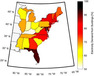
Figure 1 The percent of electricity demand from buildings (residential and commercial) by state for 2007. Data from EIA (www.eia.gov/electricity/data/state/).
Download figure:
Standard image High-resolution imageIn this work, we evaluate the response of health-relevant air emissions to climate via building energy use. Past studies have shown that air quality, especially tropospheric ozone (O3) worsens during hot weather events, because of temperature-dependent emissions, as well as meteorological and chemical processes (Jacob and Winner 2009). For example, emissions of biogenic volatile organic compounds, precursors to O3 formation, increase in warmer weather (e.g. Guenther et al 1993, Guenther et al 1997, Isebrands et al 1999, Lee and Wang 2006, Lerdau et al 1997). Climate-related emissions perturbations interact with climate-dependent chemical and transport processes, such as pollution dispersion and stagnation (e.g. Mickley et al 2004, Tai et al 2010, Georgescu 2015), and chemical processing (e.g. Jacob 1999, Steiner et al 2010). This analysis extends from climate to emissions response; future work will evaluate the net air quality impacts of climate-related energy emission changes.
A climate-sensitivity of electricity NOx, SO2, and CO2 emissions over the Eastern US has been quantified from stack emission monitors in other work from our team (Abel et al 2017), and Drechsler et al (2005) found that nitrogen oxide (NOx) emissions increased due to increased electrical demand for air conditioning in California. This analysis complements work describing the air quality co-benefits of energy efficiency measures in the current climate (e.g. Akbari et al 2001, Levinson and Akbari 2010), and outlines a methodology for coupling existing climate, building, and electricity dispatch models to address a range of issues related to building energy demand and EGU emissions.
We present a process-based modeling system to quantify the impact of increased temperatures on building energy use and electricity emissions. Our approach highlights the sensitivity of electricity emissions to ambient temperature, and provides a methodology to assess climate, technology, and policy scenarios. In this linked modeling framework, climate model data was used as input to a regional building energy model, and simulated building energy demands were used as input to a power sector model to project changes in hourly NOx and SO2 emissions. Our approach complements higher-resolution building energy demand models (e.g. Gutiérrez et al 2013) with the potential to assess building energy impacts over multi-state scales corresponding state and national air quality management, as well as regional energy planning initiatives.
We focus on the Eastern US, comparing reanalysis data for a present year with a mid-21st century scenario. We assume static building weatherization, and modest emissions-mitigation in the electricity sector. The overall change in climate evaluated represents summertime average temperature increase between 1 and 5 C across the domain (details provided in appendix A available at stacks.iop.org/ERL/12/064014/mmedia). These changes are consistent with high-warming, low-mitigation assumptions, and are intended to capture the upper-end of potential climate impacts on building energy use and air quality emissions.
Calculated power plant emissions are well suited for integration into air quality models for further assessment of ambient concentrations, population exposure, and health outcomes. Such atmospheric modeling and health impact modeling is beyond the scope of the present study. Here, we focus on emissions modeling results, and further discuss approaches and challenges for integrating energy, air quality and health assessment models.
2. Methods
In this study, we examine how buildings and power plants across the Eastern US might respond to significantly warmer regional weather. As illustrated in figure 2, this work has three components: (1) selecting present and future climate scenarios and extracting associated meteorological data, (2) simulating building response to ambient temperature and estimating the aggregate electricity demands, and (3) modeling power-plant response to increased electricity demands and other changes to the electricity supply portfolio. We considered two scenarios across each component:
- The reference case is developed to reflect present-day conditions, developed from a combination of weather and electricity demand conditions from 2007 and more current data (circa 2010) on building stock and power plant characteristics for the Eastern US.
- The mid-century warm climate (MCWC) adapted case reflects a climate future that is at the warmer end of climate projections for mid-21st century over the Eastern US. Although temperature changes in the MCWC case, building stock and power plant technology is the same as in the reference case, except insofar as electricity generation infrastructure has expanded to meet increased power demands.
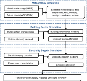
Figure 2 Project analysis flow diagram.
Download figure:
Standard image High-resolution image2.1. Current and future meteorology
Meteorology for the reference case was obtained from the National Center for Climate Prediction (NCEP) North American Regional Reanalysis (NARR). NARR data are available from 1979 through the present, with a data output every 3 hours, and a 32 km by 32 km horizontal resolution.
Meteorology the MCWC case was taken from the North American Regional Climate Change Assessment Program (NARCCAP, Mearns et al 2012). NARCCAP simulations are generated by Global Climate Models (GCMs) downscaled by Regional Climate Models (RCMs) to a 50 km × 50 km horizontal resolution, with output available every 3 hours between 2041–2070. Historic and future summer average temperatures over the Eastern US from the NARR and NARCCAP archives are included as appendix A.
Among model simulations in the NARCCAP archive, average, maximum, and minimum temperatures vary up to 10 C for any given summer, with most models overestimating historic summer maximum temperatures and underestimating historic summer minimums. Overall, we found the Weather Research and Forecasting model (WRF; Skamarock and Klemp 2008)—Community Climate System Model (CCSM; Collins et al 2006) model-pairing most closely represented historic (1979–1999) summer temperatures (Harkey and Holloway 2013).
In selecting simulated future conditions from the NARCCAP archive, our objective was to examine the potential energy and emissions impacts of a significantly warmer climate future. Among RCM-GCM model pairings in the NARCCAP archive, average future summer temperatures across the Eastern US range from 20.9 C to 31.91 C (appendix A). The warmest future summer from our selected model pairing (WRF-CCSM) is in the model year 2069; the increase in average temperatures over our study domain from 2007 (NARR) to 2069 (WRF-CCSM) is shown in figure 3. Average temperatures increase by over 1 C across much of the Eastern US, with the greatest increases (over 5 C, figure 3(b)) where historic average temperatures were less than 25 C (figure 3(a)). The selected model and year's average ozone-season (May–September) temperature is shown in context of other models over time in figure 4 to provide context for the interpretation of results and comparison with other models and years, including historic temperatures from 2010–2014. Average temperatures for these years are also shown in the context of NARCCAP simulations.
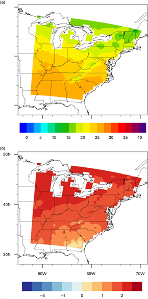
Figure 3 2007 summer (June, July, August) average temperature from the NARR dataset, top; difference between 2069 summer average temperature from the WRF-CCSM model pairing (from NARCCAP) and 2007 NARR summer average, bottom. All temperatures in degrees Celsius.
Download figure:
Standard image High-resolution image
Figure 4 NARCCAP models and respective average summer temperatures. The year chosen for analysis is represented by a yellow point. It is the hottest year from the best performing model. Range of summer average temperatures from 2010–2014, according to the EPA AVERT model, are shown with blue band.
Download figure:
Standard image High-resolution imageFor building energy use simulations, we took daily averages of downwelling shortwave radiation, cloud fraction, temperature and dewpoint temperature at 2 meters above ground, relative humidity at 2 meters above ground, surface pressure, wind speed and wind direction at 10 meters above ground, snow cover, and precipitable water from both NARR (2007) and the WRF-CCSM (2069) datasets. We interpolated the NARR data to the coarser WRF-CCSM grid for consistency across spatial scales.
We use two different climate data sets–NARR for present and NARCCAP/WRF-CCSM for future–as inputs to the building model simulation. Data from NARR supports validation of results for the present; Projections from NARCCAP provide a future climate simulation with physically consistent spatial and temporal variability in temperature, humidity, and related metrics.
The difference between the two data sets does not reflect processes in a particular climate model, given the difference in model structures. Rather, they represent two physically consistent versions of Eastern US climate appropriate for calculating building energy use.
The WRF-CCSM simulation was selected based on its correspondence with summertime mean temperatures in the Eastern US, so the difference between NARR (present) and the WRF-CCSM simulation (future) is similar to the present versus future average temperatures in WRF-CCSM. As shown in appendix A, NARR is typically cooler than WRF-CCSM summer maximum temperatures, and warmer than WRF-CCSM minimum temperatures, such that the calculated impacts of hot temperatures on building energy use are expected to be greater than would be calculated from a comparison of current and future climate from the WRF-CCSM model directly.
2.2. Building sector simulation
Our approach to modeling the demand response of Eastern US building stock to weather complements related studies (Crawley 2003, Franco and Sanstad 2008, Lu et al 2010, Lin et al 2011, Dirks et al 2015). Following Schuetter et al (2014). We developed a modeling process, named the Regional Building Energy Simulation System (RBESS), that merges state-of-the-art building energy modeling techniques with regional building stock characteristics to simulate climate impacts on building energy performance at different scales. Building stock characteristics and meteorology data (with driving variables including dry bulb temperature, humidity and solar radiation) served as inputs to RBESS, which then simulated the heat transfer and mechanical operation interactions of the buildings with the ambient environment. Regional differences in temperature, humidity, and solar radiation, and their impacts on energy loads are captured by simulated zone (the discussion in this manuscript focuses on temperature as a proxy for the multivariate climatic changes included in the simulation). While RBESS can be used to examine adaptive measures, our assumption for this study was that current Eastern US building stock remains static, i.e. we assumed no retrofitting of existing buildings and no construction of new buildings, and no population growth.
Data from three separate surveys were used to characterize the building stock of the Eastern US; the Commercial Buildings Energy Consumption Survey (CBECS 2003), the Residential Energy Consumption Survey (RECS 2009), and the Manufacturing Energy Consumption Survey (MECS 2006). Data from the surveys were used to characterize the building types and energy use within five eastern US Census Regions: New England (Connecticut, Maine, Massachusetts, New Hampshire, Rhode Island, and Vermont), Middle Atlantic (New Jersey, New York, and Pennsylvania), South Atlantic (Delaware, District of Columbia, Florida, Georgia, Maryland, North Carolina, South Carolina, Virginia, and West Virginia), East South Central (Alabama, Kentucky, Mississippi, and Tennessee), and East North Central (Indiana, Illinois, Michigan, Ohio, and Wisconsin).
We developed 17 prototype buildings using the eQUEST energy modeling software (eQUEST 2010). Each building model was parameterized with common building features, e.g. heating, ventilation, air conditioning (HVAC), lighting, etc. We did not vary common building features by region. Prototype building energy models were calibrated using American Society of Heating, Refrigerating and Air-Conditioning Engineers Guideline 14 (ASHRAE 2014) to represent energy-use profiles for each US census division. In order to simplify the analysis, several of the smaller sectors were left out of the final characterization. These smaller sectors represented 3.7% of the overall energy usage. A scaling factor within each region and for each energy model was used to scale individual prototype building energy to the region. Scaling factors were based on the total energy consumption within the region and energy sector as provided by the survey data. Each survey data set represented a different year so we scaled total energy consumption to a baseline year (2007) based on the proportion of energy used by each building type for the survey year reported. We did not consider changes in energy consumption by building stock between years.
Prototype models were set up in a batch system processor that uses the DOE-2 (DOE2) building energy simulation program. Building simulation was first performed for a 2007 historic reference year, using NARR meteorology. Daily weather was spatially averaged over each of the six regions except for the South Atlantic. Due to the variety of latitudes contained within the South Atlantic region, daily averaged weather over this large region was split between North Carolina and South Carolina. Tables included as appendix B summarize prototype building types and energy use, respectively.
The historical electricity demand data for 2007 was based on US EPA compilation of Federal Energy Regulatory Commission (FERC) load data for each FERC-identified balancing area (USEPA 2014a). To conform to the same footprint as building-stock data, balancing areas loads were transposed onto state and census division boundaries, forcing demand to conform to historic state-level consumption estimates (USEIA 2007), and thereby approximating hourly electricity demands for each state and region. For model calibration, RBESS was used to simulate the energy performance of Eastern US building stock using 2007 weather and electricity data. Results for individual prototypes were compared with the DOE's Building Performance Database (USDOE 2012) and simulated electricity demand was compared to historic electricity demand profiles.
Following the simulation and calibration of a reference year, RBESS was used to simulate the performance of Eastern US building stock, using the same building stock prototypes, in response to MCWC weather data. As with the building demand modules used by the DOE/EIA for projecting energy use, we assumed no significant changes in building technology or consumer behavior. We also assumed no changes to non-building related energy use, and isolated only the change in electricity demand from building response to warmer weather.
2.3. Electricity supply simulation
To simulate the operation of Eastern US power plants and their associated emissions, we used MyPower, a load duration curve (LDC) electricity dispatch model, used previously to estimate changes to air quality occurring because of changes to power sector resources (Plachinski et al 2014).5 LDC models remain in common practice for long-term evaluation of power sector emissions, including US EPA's use of the Integrated Planning Model (IPM) to evaluate proposed air quality rules (USEPA 2014a), and the Midwest Independent System Operators evaluation use of the Electric Power Research Institute's EGEAS model (MISO 2014) to evaluate the proposed Clean Power Planning Rule (US Federal Register 2014). LDC models divide electricity demand (i.e. load shape) into a set of smaller segments and then estimate each power plant's contribution to those load segments. A dispatch algorithm sorts the plants in order of least-cost operation, based on each facilities' thermal efficiency, fuel price, variable operation and maintenance costs, production credits. Operational constraints and/or regional power interchange may also be included. For this study, we used four-segment LDCs constructed for both the historic 2007 electricity demand as well as for the MCWC mid-21st century electricity demand. Twenty-six 'local' electricity systems were constructed to represent each of the 26 Eastern US states. We assumed interchange of power via a single limited-capacity tie-line between each local system and a regional set of neighboring states. This single-tie interchange is similar to the approach used by the Oak Ridge Competitive Electricity Dispatch (ORCED) model (ORNL 2010).
Data for power plant operational characteristics was derived from the National Electric Energy Data System (NEEDS), available as part of US EPA's Power Sector Modeling Platform (USEPA 2014a). This NEEDS version included actual power plant construction through 2011, including heat rates and emission rates, as well as some post-2011 power plant additions, based on anticipated construction. Power plant data was modified to reflect actual emission rates and heat rates as reported in US EPA's Clean Air Markets Database (CAMD) (US EPA 2014b). In addition, we incorporated operational constraints to de-rate each power plant's available generating capacity to reflect planned and forced outages for fossil-fuel generators, and to reflect a typical production capacity for renewable sources, based on historic operations (USEIA 2011).
As a means of quality assurance, we evaluated the power-sector model performance by comparing simulated 2007 results to historically reported data for fossil fuel power plants in the eastern US. To do so, we reverted the database to include only power plants operating during 2007 and assuming 2007 emission rates and heat rates. The facility level estimates of generation and emissions were compared to historically reported CAMD values.
Figure 5 provides a plant-by-plant comparison for the East North Central region of Indiana, Illinois, Michigan, Ohio, and Wisconsin, a region often referred to as the Upper Midwestern US. The other four regional plots are included as appendix C. These plots compare generation (GWh) and emissions of CO2, NOx, and SO2 by facility, with simulated results on one axis and historically reported values on the other such that data points falling on the 1:1 slope line indicate perfect agreement. We use Microsoft Excel's (v. Office 2010) trendline function to estimate the overall agreement. The R2 values for each region are shown in table 2. With 19 of 20 R2 values at 0.87 or greater, these results demonstrate good agreement between modeled estimates and historically reported performance.
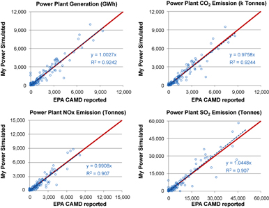
Figure 5 Comparison of simulated 2007 results to historically reported 2007 values for fossil fuel power plants in the East North Central region.
Download figure:
Standard image High-resolution imageElectricity supply conditions were constructed to reflect both the reference and MCWC scenarios. Electricity supply for the reference case reflects current conditions by updating the NEEDS-reported power plant emission factors and heat rates to 2013 values using CAMD reported values. Reference case emissions results are based on this characterization of supply in response to electricity demands (LDCs) constructed from 2007 data. The reference is intended to represent circa 2010 electricity supply, rather than a precise study year, in response to realistic demand conditions constructed from historical conditions. The electricity supply for the MCWC-adapted case was designed to reflect a reasonable basis for future electricity supply. We assumed that renewable portfolio standards (RPS) were satisfied through a combination of technologies, and primarily those that targeted wind power, based on state-specific standards reported in the DSIRE database (USDOE 2013).
The net changes to nuclear power are based on the construction of the 11 new reactors that currently have existing construction applications at the Nuclear Regulatory Commission (US NRC 2013) and the total retirement of the existing nuclear fleet by mid-century, as should be anticipated given existing operating licenses. We also assumed the MCWC-adapted case maintained 'resource adequacy,' such that installed generating capacity was required to exceed the highest MCWC demand by 15%. The remainder of the required power plant capacity was assumed to have been supplied through the construction of natural-gas power plants, of which 70% were combined-cycle and 30% single-cycle technology. Operational characteristics for existing power plants were held constant with the reference case, while characteristics for new power plants were based on power-plant-technology assumptions from the Annual Energy Outlook (USEIA 2012).
Emissions were calculated by MyPower for each emitting power plant as a function of electricity generated, seasonal-specific heat rate (fuel required per unit generated), emission rate (emission mass per unit of fuel input), and air pollution control efficiency. The results section illustrates these emissions both on a plant-by-plant basis, as an aggregated hourly profile by state, and as regional seasonal totals.
To generate hourly emissions estimates, we compared the hourly load projection (a chronological succession of hourly loads) to the MyPower-estimated hours of operation for each EGU. Each EGU was assumed to operate during each hour of the season for which the load rank (rank of the current hour relative to all hours of load) was less than the EGU's total hours of operation. For example, a power plant estimated to operate for 500 hours during the peak season was assumed to be operating during the 500 highest hours of electricity demand (i.e. for each hour of the season with load rank less than or equal to 500, this power plant is assumed to be operating and emitting). It should be noted, that this approach ignores the short-term operational constraints of the power grid. In real-world operations, grid operators limit the rate at which power plants ramp up or down in response to changing load, and further avoid toggling power plants on for short periods of time. These transient considerations are typically modeled using hourly production simulation tools, generally considered too onerous for long-term research applications. For long-term studies where an LDC models are appropriate, the straightforward approach used here is a simple means to allocate seasonal emission estimates into temporally and spatially explicit inventories. An extended discussion of the challenges and trade-offs between available modeling approaches is provided in US EPA's Carbon Pollution Emission Guidelines for Existing Stationary Sources: Electric Utility Generating Units (Federal Register 2014).
3. Results
The integrated modeling approach, described above, supports our consideration of the relative impact of warmer weather on electricity sector emissions. Here we present model results for a case study that combines the weather, building stock, and an energy supply scenario. Results are divided to discuss the building energy response to warmer weather and the power-sector response to changing building energy use.
3.1. Building energy response to warmer weather
Simulations with RBESS provide hourly electricity demand for each census division of the US, shown for the East North Central region in figure 6 (for the full year). Plots for all Eastern US regions are included as appendix D. During the summer months, future climate yields a major increase in electricity demand, over nearly every hour of every day. The northern regions, which tended to experience greater increases in temperature and cooling-degree-days, tended to experience greater increases in peak electric demand. Figure 6 shows graphically the basis for the values in table 1, which reports regional differences in the response of electricity demand to future climate. The largest impact occurs in the East North Central Region (50% increase in peak demand, shown in figure 6) and the smallest impact occurs in the South Atlantic region (7% increase in peak demand, shown in appendix D).
Table 1. Change in regional peak season (1 May–30 Sept) electricity demand between 2007 historic and simulated MCWC conditions.
| Seasonal electricity demand (1000 GWh) | Peak electricity demand (GW) | |||||
|---|---|---|---|---|---|---|
| Region | Present | MCWC | Change | Present | MCWC | Change |
| East North Central | 279 | 321 | 15% | 115 | 173 | 50% |
| East South Central | 163 | 179 | 10% | 71 | 96 | 36% |
| Middle Atlantic | 181 | 197 | 9% | 82 | 110 | 35% |
| New England | 54 | 59 | 9% | 24 | 30 | 26% |
| South Atlantic | 399 | 393 | −2% | 176 | 189 | 7% |
| Total | 1076 | 1149 | 7% | 438 | 576 | 32% |
Table 2. R-squared values for historic versus simulated results for 2007 by region.
| R2 | n | GWh | CO2 | NOx | SO2 |
|---|---|---|---|---|---|
| East North Central | 357 | 0.92 | 0.92 | 0.91 | 0.91 |
| East South Central | 106 | 0.92 | 0.95 | 0.88 | 0.96 |
| Middle Atlantic | 266 | 0.89 | 0.92 | 0.93 | 0.98 |
| New England | 154 | 0.87 | 0.87 | 0.80 | 0.96 |
| South Atlantic | 321 | 0.90 | 0.92 | 0.93 | 0.95 |
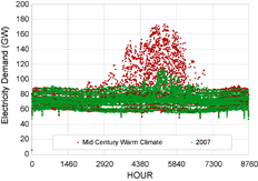
Figure 6 East North Central Regional electricity demand under present (2007) conditions and RBESS simulated conditions with future (MCWC) weather data. See also appendix A.
Download figure:
Standard image High-resolution imageThe largest increases in peak demand appear to be driven by increases in energy use in the residential sector occurring in the afternoon between the hours of 4:00 pm and 8:00 pm. The average diurnal cycles for both the reference (2007 NARR) and MCWC (2069 WRF-CCSM) cases are shown in figure 7, along with the regional average maximum and minimum temperatures at each time of day. Future summer temperatures increase across all hours of the day, with the greatest average increase seen in daytime maximum temperatures (9.8 C).
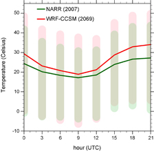
Figure 7 Average seasonal diurnal cycle for the reference (NARR 2007) and MCWC (WRF-CCSM 2069) cases with a range of temperatures shaded.
Download figure:
Standard image High-resolution imageAcross the region, RBESS calculates a 7% increase in seasonal electricity requirements, and a 32% increase in non-coincident peak demand. These findings are supported by past research showing an annual US average increase in source electricity building demand of 6% from 2008–12 to 2060–79 (Huang and Gurney 2016). Non-coincident peak demand accounts for the total magnitude of changes in peak demand, occurring across multiple regions, with peak conditions occurring at different times.
During the cold-season months, there is little difference in energy demand between the present and future climate scenarios. Whereas space cooling is powered by electricity, natural gas plays a more important role in space heating. Because this study focuses on electricity generation and demand, potential reductions in natural gas and fuel oil for heating are not included. In many southeastern US states, electricity production is the main source of space heating, and our simulations suggest a slight decrease in demand during winter months in the Southeast under the MCWC scenario (appendix D). However, our calculations indicate that increases in summer electricity demand far exceed decreases in winter demand in all regions.
3.2. Power-sector response to changing building energy use
We examine the change in regional power plant emissions as they respond to warmer weather. All results shown are from May 1 to September 30, which represents the 'ozone season' for air quality planners and 'peak season' or 'cooling season' for electricity planners, during which building electricity demands are generally greatest.
Emissions impacts are a function of electricity supply, or fuel mixture (i.e. the portfolio of fuels used by the total fleet of EGUs to meet demand), illustrated in figure 8. The net increase in electricity generation needed to meet building cooling demands is visible in figure 8, by comparing the reference case to the MCWC case. Total changes to electricity generation are generally proportional to the changes in demand shown in table 1.
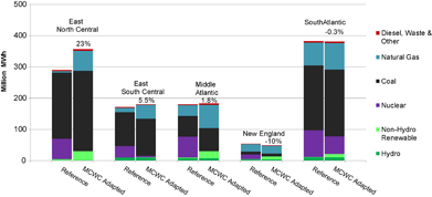
Figure 8 Simulated electricity supply mix for reference case and MCWC-adapted cases for the peak/ozone season (1 May–30 Sept).
Download figure:
Standard image High-resolution imageAs shown in figure 8, the most pronounced increase in generation under the future climate scenario occurs in the East North Central region at 23%. Smaller increases are calculated for the East South Central (5.5%) and Middle Atlantic (1.8%) regions. Reductions are calculated in the South Atlantic (−0.3%), and to a more significant degree in New England (−10%), where a loss of nuclear generation capacity results in increased reliance on imported power.
In all regions, the reliance on coal and gas-powered electricity increase. This occurs in part due to higher electricity demands, and because existing nuclear facilities are assumed to retire. The energy contribution of retired nuclear is only partially compensated for with new nuclear construction in the South Atlantic and East South Central regions. The other regions show increasing reliance on renewable resources as a result of RPS requirements. In the MCWC case, coal remains the largest source of electricity supply. Natural gas consumption increased substantially in all regions, but particularly in the Middle Atlantic and in New England where it is the largest contributor to the regional fuel supply.
Figure 9 compares calculated emissions with reported emissions for 2007 and 2013. Considerable emission reductions occurred between 2007 and 2013, particularly for SO2 and NOx. While much of this is due to pollution control additions, the reductions in CO2 (which remains uncontrolled) indicate that some of the historic reductions are due to fuel mixture changes, e.g. increased contributions from natural gas and renewable power sources. The simulated reference emissions fall between the 2007 and 2013 emission levels in the East North Central, East South Central, and South Atlantic regions, and are somewhat higher than historic emissions in the Middle Atlantic and New England regions.
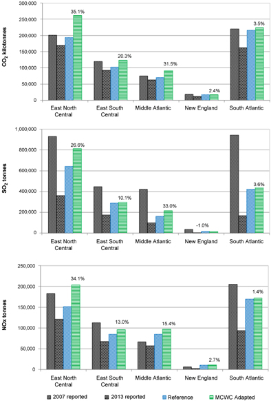
Figure 9 Historic and simulated regional emissions for the reference case and MCWC-adapted case (1 May–30 Sept ozone season).
Download figure:
Standard image High-resolution imageOf primary interest for this study is the relative increase in emissions occurring between the reference case (in blue in figure 9) and the MCWC-adapted case (in green). The resulting regional summer emissions are shown in figure 9. In response to MCWC electricity demand, emissions increase 2.4% to 35% for CO2, −1% to 27% for SO2, and 1.4% to 34% for NOx. The general trend is consistent for all three pollutants with the largest increases occurring in the East North Central, East South Central, and Middle Atlantic regions, and only slight changes occurring in New England and South Atlantic regions. Emissions increases in these regions are larger than the net increase in electricity demand (table 1), indicating an increased reliance on less-efficient and higher-emitting power plants. The net change to emissions can be related both to changes in demand and to the reliance on coal and natural gas reliance discussed above and visible in the figure 8 fuel-mixtures graphic. Emissions changes were negligible in the South Atlantic due to limited changes in both demand and fuel mixture (see figure 8). Emission changes in New England were also negligible, as the total contributions from coal and natural gas were similar in both the reference and MCWC case (see figure 8).
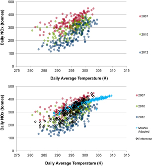
To illustrate the temperature dependency of NOx emissions, figure 10 merges historic emissions and temperature data for Ohio, a state in the East North Central region. Figure 10 shows total daily NOx tonnes as reported by EPA CAMD (USEPA 2014b) against daily average temperatures for 2007, 2010, and 2012. Two trends are clearly illustrated by the historic data. First, NOx emissions increase with increased temperature. Second, NOx emissions have successively declined between 2007 and 2012. Temperature dependency for the reference case shows a temperature dependency similar to that of 2010 historic data in both slope and magnitude. The MCWC case also shows a similar temperature dependency, yet with a more shallow slope and more tightly banded data points. In the MCWC case, 43 days have higher average temperatures than the historic years shown. The shallower slope indicate that the peak demands are being satisfied by new natural-gas power plants, and not by older less-efficient plants, which would yield an increasingly upward slope. This also explains why daily emissions in the MCWC case are more tightly banded, because generation from new lower-emitting natural-gas increasingly follows load, thereby diminishing the frequency with which large coal-fired generators toggle on and off.
Figure 10 Temperature dependency of historic and simulated NOx emissions for Ohio (daily tonnes) for 1 May through 30 September.
Download figure:
Standard image High-resolution image
4. Discussion
This study characterizes the potential impact of heat-related increases in electricity demand on health-relevant air emissions. Our analysis considered how electricity sector emissions might respond to a mid-century climate on the warmer end of model assessments. Results are consistent with expectations that warmer temperatures lead to higher levels of building energy use, and higher levels of associated electricity emissions. Building energy modeling results were similar to those expressed in the National Climate Impact Assessment (Melillo et al 2014), with net electricity use from buildings expected to increase in a warmer climate.
We find that climate change projections are an important consideration in meeting future electricity needs, consistent with Schaeffer et al (2012). In response to summer-average temperature increases ranging from 1 C to 5 C across the domain (with associated changes in other weather variables), simulated building energy loads increased electricity demand by 7%, with a 32% increase in non-coincident peak demand. The states of Indiana, Illinois, Michigan, Ohio, and Wisconsin, collectively the East North Central region, show the greatest sensitivity of energy use to climate among the study regions.
In response to greater building energy demands, simulated power sector emissions increased, though the magnitude of emissions is dependent on energy supply assumptions. Common assumptions for power-sector modeling require that capacity reserves are maintained, i.e. require that supply-side generating capacity exceeds peak demand by a fixed percentage. The impact of this assumption on emissions results should be closely scrutinized. Modeling the same demand conditions with lower capacity reserve, as might occur if infrastructure planning does not take account of climate projects, could force older and higher emitting units to respond to the growing demand.
While the overall trends from the building energy modeling results are consistent with expectations, there remains considerable variability among regions compared to other similar studies (e.g. Sailor 2011, Dirks et al 2015). While we assumed building stock to maintain static characteristics, dramatic increases in cooling demands would be more likely to incentivize both conventional and advanced building-mitigation strategies, including consumer behavioral approaches. Building efficiency efforts focused on cooling-efficiency equipment and interruptible load programs represent conventional approaches. Energy storage systems or demand response programs, which could dramatically affect building demands during hot weather, may warrant more serious consideration where climate risk is more dramatic, as in the simulated meteorology for the East North Central region. Nonetheless, for decision makers and stakeholders to make use of such results, it needs to be in a form that is actionable at the building level. Major questions remain as to which energy efficiency and conservation strategies are best for addressing climate resiliency in buildings. Gunasingh et al (in press) show how climate change can alter the impact of specific equipment and energy efficiency measures on the energy use of a building suggesting that future building designs need to start incorporating future climate files. Coley et al (2012) suggest modeling with the 50th percentile of climate change data and examining 'hard' mitigation measures to reduce expected climate risk and using 'soft' approaches for greater than expected changes.
Assuming that the electricity infrastructure expands to ensure an adequate capacity reserve under a warmer climate, with limited changes to current generation resources, we calculate a 16% increase in emissions of NOx and 18% increase in emissions of SO2, for the simulated climate scenario. We assumed conservative increases in renewable and nuclear power and a static state (no assumed retirements) for existing fossil fuel power plants. These fuel supply assumptions were ultimately insufficient to reduce emissions growth. Recent 'real world' market conditions reflect an accelerating transition away from coal and toward natural gas and renewable resources, which would lower emission rates (simulated and actual) for all pollutants. As with energy, the East North Central region shows the greatest response of emissions to climate among the study regions.
The linked modeling system presented here leverages process-based relationships to evaluate environment, technology, and policy impacts on air emissions. However, the expense of this system limits the number of alternate scenarios that can be tested. To consider the potential of alternate building efficiency measures to compensate for climate-related electricity demand, a reduced form model like the US EPA's AVoided Emissions and gene Ration Tool (AVERT) offers a complementary analysis method. AVERT at present only includes present-day scenarios (historical years 2010–2014), and it can be used to consider energy efficiency scenarios over a limited number of future years. When applied to our study region over the Eastern US, AVERT suggests that emissions decreases from energy efficiency are proportionally similar (±10%) to reductions in generation. As such, the increased emissions associated with a warmer climate may be offset by efficiency measures, although the details of implementation would require a more directly comparable analysis framework.
It is also worth noting the challenge of conducting climate impacts assessment modeling for systems that vary on short spatial and temporal timescales like electricity production, air emissions, and ambient air quality. Whereas climate impacts analysis generally expects a 30-year simulation period to capture system change, high-resolution simulations of climate-dependent systems are often not feasible over such a long period. To reconcile these competing demands, we selected a single year for analysis from a multi-year, multi-model archive. This approach allowed us to focus on a single future year, while framing results in the context of future climate uncertainty. There is no 'right' way to select a future model year, but by documenting the criteria used for selecting a study year/simulation, climate impacts results for the simulated conditions may be contextualized relative to other model years and simulations (figure 4).
There is a high level of spatial and temporal heterogeneity in the response of weather to climate, of building energy use to weather, of power plant generation to building energy use, and of emissions to generation. This work highlights the potential impact of climate change on energy use and emissions, with a focus on the ozone season, when warming temperatures would most directly impact electricity demand and exacerbate air pollution in the summer months. This methodology may be extended to a broader set of scenarios, sensitivities, and probabilistic outcomes, and may support the development of reduced form models for more widespread policy evaluation.
Acknowledgments
This work was supported by the National Institutes of Health Grant 1R21ES020232-01, and a Vilas Mid-Career Award to Tracey Holloway and a Romnes Faculty Fellow award to Jonathan Patz from the University of Wisconsin–Madison. Additional support was provided by the Wisconsin Energy Institute at the University of Wisconsin–Madison, and the Nelson Institute for Environmental Studies through the Center for Sustainability and the Global Environment (SAGE). Ryan Kladar provided conception and contributions to figure 10, with support from the NASA Air Quality Applied Sciences Team. Vijay Limay provided valuable project coordination. Daegan Miller provided editing and manuscript contributions.
We wish to thank the publicly funded organizations that have provided data and models used in this study. In particular, the Environmental Protection Agency provided data from the Clean Air Markets Database, and the AVERT Model. The North American Regional Climate Change Assessment Program (NARCCAP) for providing the data used in this paper. NARCCAP is funded by the National Science Foundation (NSF), the US Department of Energy (DoE), the National Oceanic and Atmospheric Administration (NOAA), and the US Environmental Protection Agency Office of Research and Development (EPA). NCEP Reanalysis data are provided by the NOAA/OAR/ESRL PSD, Boulder, Colorado, USA, from their Web site at www.esrl.noaa.gov/psd/
Footnotes
- 5
Dr. Meier has an ownership interest in Meier Engineering Research LLC, which owns the MyPower model used in this study.