

Abstract
Water scarcity adversely affects ecosystems, human well-being and the economy. It can be described by water scarcity indices (WSIs) which we calculated globally for the decades 1981–1990 and 2001–2010. Based on a model ensemble, we calculated the WSI for both decades including uncertainties. While there is a slight tendency of increased water scarcity in 2001–2010, the likelihood of the increase is rather low (53%). Climate change played only a minor role, but increased water consumption is more decisive. In the last decade, a large share of the global population already lived under highly water scarce conditions with a global average monthly WSI of 0.51 (on a scale from 0 to 1). Considering that globally there are enough water resources to satisfy all our needs, this highlights the need for regional optimization of water consumption. In addition, crop choices within a food group can help reduce humanity's water scarcity footprint without reducing its nutritional value.
Export citation and abstract BibTeX RIS

Original content from this work may be used under the terms of the Creative Commons Attribution 3.0 licence. Any further distribution of this work must maintain attribution to the author(s) and the title of the work, journal citation and DOI.
Introduction
While humanity consumes water volumes below the planetary boundary (Steffen et al 2015), our use of freshwater resources is still unsustainable, as much water is consumed in highly water scarce regions. With a stabilisation target of a water scarcity index (WSI) ≤ 0.5 for all individual watersheds, we would have to reduce our global water scarcity footprint by about 50% (Ridoutt and Pfister 2010). However, the share of water consumed from unsustainable resources is predicted to increase in the future (Wada and Bierkens 2014). Further complicating the issue, transboundary watersheds and international trade lead to impacts far distant from local consumption (Vörösmarty et al 2015). This enormous challenge we are facing points to the need for global information on water scarcity such as expressed by WSIs.
Various researchers calculated monthly WSIs (Hoekstra and Mekonnen 2011, Pfister and Bayer 2014, Scherer et al 2015) for different periods, e.g. 1961–1990. However, WSIs do not only vary seasonally, but, as a consequence of changing climate, population and lifestyles, they also vary inter-annually (Núñez et al 2015). Therefore, the WSIs have to be updated regularly. In addition, underlying global hydrological models entail high uncertainties which propagate to WSIs (Scherer et al 2015), but these are hardly reported. Consequently, the following objectives were pursued in this study: (i) to update WSIs to a more recent period; (ii) to assess uncertainties; (iii) to investigate intra- and inter-annual as well as regional trends; and finally (iv) to analyse the role of regional optimization and crop choices as alternative approaches to alleviate water scarcity globally.
Methods
Calculation of WSIs
WSIs in this work were estimated according to the method by Pfister et al (2009) which was originally developed for annual WSIs considering total water resources:
where WTA* is a modified withdrawal-to-availability ratio accounting for temporal variation in precipitation and flow regulation (Pfister et al 2009). It can be replaced by a modified consumption-to-availability ratio (CTA*). The coefficient c was tuned to result in a WSI of 0.5 for a WTA of 0.4 as the boundary between moderate and severe water scarcity, while the thresholds from low to moderate and severe to extreme are at a WSI of 0.1 and 0.9. We modified c for different water origins (total, surface or groundwater resources), temporal resolutions (annual or monthly) and if water withdrawal and water consumption are used (Schakel et al 2015). Annual averages of monthly WSIs and global and country averages were each weighted by consumption or withdrawal, respectively. In addition, a global average WSI was weighted by human population (Doxsey-Whitfield et al 2015).
Although many studies on water scarcity incorporate water withdrawal instead of water consumption (Pfister et al 2009, Pfister and Bayer 2014), we use the latter as was already done by other scientists (Hoekstra and Mekonnen 2011), because it better reflects physical water scarcity (Scherer et al 2015). By focusing on water consumption, we only take into account water quantity despite the fact that water withdrawn and released back to the environment might be of lower quality and unusable for some users (Scherer et al 2015). This can be justified by separate methods being available to address water degradation such as from phosphorus emissions (Scherer and Pfister 2015), thermal emissions (Pfister and Suh 2015) or acidification (Roy et al 2014).
We use six global models for river discharge, four for groundwater recharge, six for precipitation and three for water use to estimate WSIs at a spatial resolution of 0.5°. Water availabilities and precipitation were obtained from the Earth2Observe project (EartH2Observe 2015). Water use was taken from Wada et al (2014b), Flörke and Eisner (2011) and Pfister and Bayer (2014). Wada et al (2014b) only provided water withdrawal which was converted to water consumption by applying a consumption-to-withdrawal ratio derived from the data of Flörke and Eisner (2011). By contrast, Pfister and Bayer (2014) only provided water consumption for crop production, which was converted to water withdrawal by applying irrigation efficiencies (Döll and Siebert 2002). Irrigation water use from Pfister and Bayer (2014) and water use of sectors other than irrigation from Flörke and Eisner (2011) were combined to one dataset. Rivers were considered as strongly regulated when the upstream area of the nearest upstream dam (Lehner et al 2011) covered more than half the total upstream area (Wu et al 2012).
Uncertainty assessment and model validation
Multiple models were available for all the three major input parameters required to calculate WSIs: water availability, water consumption and precipitation. Based on the means and standard deviations among the models, probability distributions were derived and used for latin hypercube sampling. The uncertainty among the models was subsequently propagated to WSIs by Monte Carlo simulations. While as few as 100 iterations should be sufficient (Kennedy et al 1996, Steen 1997), we performed 1000 iterations following the recommendation of Steen (1997). We assumed a normal distribution for the estimates among the different models.
We described the uncertainty in the resulting WSIs by the coefficient of variation (CV), the comparison between the deterministic WSI and the mean and median of the probabilistic WSIs as well as the k-value (dispersion factor). The k-value was originally defined as the root of the ratio between the 97.5th and the 2.5th percentile (Slob 1994), but its robustness was increased by averaging it with the root of the ratio of the 97.5th percentile to the median and of the median to the 2.5th percentile (Núñez et al 2015).
Beside uncertainty assessment, model validation is crucial to evaluate the model performance. Therefore, monthly river discharge was validated against observed river discharge from the Global Runoff Data Centre (GRDC 2013) for 186 watersheds (supplementary information). The model performance was evaluated by multiple criteria including the Nash–Sutcliffe efficiency, percent bias (PBIAS) and normalised root mean square error (NRMSE) as recommended by Moriasi et al (2007). It was subsequently related to the aridity index (Zomer et al 2008) to test the hypothesis that more arid regions perform poorer (Scherer et al 2015).
Total water withdrawal was validated against data from the AQUASTAT database (FAO 2015a) for 152 countries (supplementary information). Given that no monthly time series are available for validation, the model performance was only evaluated by the percent bias (PBIAS; Moriasi et al 2007).
Trend analysis
Having obtained probability distributions for the two selected decades, we determined the likelihood that water scarcity is more severe in the later decade than in the earlier decade by counting true incidences of the individual Monte Carlo runs. Similarly, water availability and consumption were compared for the two decades in order to identify the major driver of any change in water scarcity. By subdividing the globe into regions of severe (WSI ≥ 0.5) and low to moderate (WSI < 0.5) water scarcity, we analysed if water scarce regions are getting scarcer in water, while water abundant regions are getting more abundant in water. Likewise, we split the year into two seasons and defined the scarce season as the six-month period with the highest monthly WSI in order to analyse if water scarce seasons are getting scarcer in water, while water abundant seasons are getting less scarce.
Furthermore, we performed the Wilcoxon–Mann–Whitney test (Mann and Whitney 1947) in order to examine if there is evidence for a significant shift between the means of two distributions and the Mann–Kendall test (Mann 1945) combined with the Theil–Sen estimate (Sen 1968) in order to investigate the significance of a trend from 1981 to 2010. Both tests are non-parametric. As such, they do not rely on the assumption of a normal distribution.
Regional optimization versus crop choice
We compared the variability in crop water consumption among crops in food groups and among countries for specific crops in order to analyse the potential of two strategies to alleviate water scarcity: regional optimization and crop choice. Regional optimization implies that producers shift production sites to more favourable locations, while it involves changing trade partners for importing consumers. Alternatively, these results can be used to focus on water productivity in less favourable areas. On the other hand, crop choice suggests a change in diet to less water critical food products without constraining the nutritional value of the diet.
Water consumption of 147 food crops from 160 countries were obtained from Pfister and Bayer (2014). The crops were assigned to eleven food groups: cereals, forage, fruits, nuts, oil-bearing crops, pulses, roots and tubers, spices, stimulants, sugar crops and vegetables (table S3). The grouping shall ensure that the crops have similar nutritional values and dietary functions and are therefore considered substitutable. The variability within regions and among crops was described by CVs weighted by crop production. For countries, the coefficients were determined for each crop and then averaged for the crops within one food group, while for crops the global averages were compared within a food group. The production of agricultural goods was derived from crop yields and areas (Monfreda et al 2008). A greater variability indicates a higher potential for optimization.
In addition to these overarching analyses, two case studies on specific crops of similar dietary functions were carried out, including the calculation of their impacts on water scarcity by applying the new WSIs. First, we examined maize, rice and wheat as major staple food crops, which together supply humanity with about half of their dietary energy (FAO 2014); and second, we examined the stimulants coffee and tea, as they are among the highest water consumers (Pfister and Bayer 2014) but only represent luxury goods. We analysed the respective three major exporting countries as well as a global production-weighted average and calculated water deprivation as the product of the WSI and water consumption, resulting in a water scarcity footprint (WSF; ISO 2014).
Crop water consumption from Pfister and Bayer (2014) are geometric means, while Pfister et al (2011) provide water consumption based on deficit irrigation, which was assumed to represent the 2.5th percentile of a lognormal distribution to account for uncertainty in irrigation water consumption. The major exporters of the products were identified based on data from the FAOSTAT database for the year 2012 and production was available for the year 2013 (FAO 2015b). The staple food crops were compared based on their calorific content as mega calories (Mcal, USDA 2015), whereas the stimulants were compared based on their caffeine content which coincides with a standard cup. The ingredients of a standard cup of coffee or tea were taken from Chapagain and Hoekstra (2007). A cup of coffee is typically 125 ml and contains 50 mg caffeine (USDA 2015), while a cup of tea is typically 250 ml and also contains 50 mg caffeine (USDA 2015). Like for WSIs, uncertainties of water scarcity footprints were propagated based on latin hypercube sampling using 1000 iterations, including the uncertainty of both WSI and water consumption.
Personal budgets
Regional optimization and crop choice represent two possible pathways to reduce humanity's water footprint. However, the global scale and the large number of actors and stakeholders engaged often leads consumers to abdicating their responsibility. In order to stimulate individuals to assume responsibility for reducing humanity's water footprint, we estimated personal budgets of water consumption for the scenario of equitable sharing of our global water resources. According to Ridoutt and Pfister (2010), we have to reduce humanity's water scarcity footprint by about 50%. Since their estimate is based on data for the period 1961–1990, we calculated the average annual water consumption for the earlier decade of 1981–1990. This decade's half water consumption is then divided by the current world population of 7.35 billion people (UN 2015) to obtain personal water budgets.
Results and discussion
Refined WSIs
Water scarcity is especially high in North Africa, the Middle East, India, the Mediterranean region, the Western coast of the United States and South America and the surroundings of Beijing in China (figure 1). Countries that are heavily affected and at the same time among the largest agricultural producers are Spain, India, Indonesia and Turkey (figure 2). The consumption-weighted average monthly WSI in the period 2001–2010 amounts to 0.51 (table 1) and this indicates that on average we are consuming water under moderate to high water scarcity, while the average person lives in an area with a WSI of 0.32. Uncertainty analyses reveal that it is 56% probable that global consumption-weighted average water scarcity is severe (WSI > 0.5) and 100% certain that it is at least moderate (WSI > 0.1). Our results further indicate that on a global level annual WSIs underestimate water scarcity (table 1) and thus highlight the importance of using a finer temporal resolution (Pfister and Bayer 2014, Scherer et al 2015). Groundwater scarcity is generally higher than surface water scarcity (table 1) and raises the question if water use can also be optimized for the source of water. However, it might be a result of the water allocation in the water use model where priority is given to groundwater in order to meet the water demand (Wada et al 2014b) and should therefore be investigated in more detail in future research. Nevertheless, Gleeson et al (2012) pointed to the overexploitation of aquifers and revealed that the aquifer area would have to be 3.5 times larger in order to sustain humanity's groundwater use and groundwater dependent ecosystem services. Such optimization endeavours should, however, be guided by local rather than global studies. Despite the high uncertainties associated with water scarcity footprints, the spatial pattern is robust, which is evidenced by a high average Spearman's rank correlation of 0.86 (median = 0.91) between the deterministic WSIs of watersheds and the 1000 probabilistic WSIs resulting from the Monte Carlo simulation.
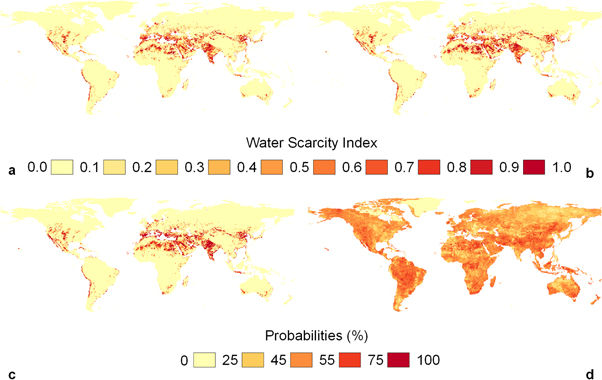
Figure 1. Monthly consumption-weighted water stress indices. (a) 1981–1990. (b) 2001–2010. (c) Probabilities of water scarcity (WSI > 0.5) in 2001–2010. (d) Probabilities of water getting scarcer from the earlier to the more recent time period.
Download figure:
Standard image High-resolution image
Figure 2. Monthly water stress indices in 1981–1990. (a) Consumption-weighted WSIs at country level. (b) Withdrawal-weighted WSIs at watershed level. (c) Withdrawal-weighted WSIs at watershed level based on data from Pfister and Bayer (2014). (d) Absolute differences between the WSIs in this study (b) and those from Pfister and Bayer (2014) (c).
Download figure:
Standard image High-resolution imageTable 1. Global consumption-weighted average water stress indices (WSIs). We considered different temporal resolutions (monthly and annual), different water origins (TOT: total, SW: surface and GW: groundwater resources) and different time periods (early: 1981–1990, late: 2001–2010). A WSI ≥ 0.5 indicates severe water scarcity. Those values are presented in bold. A coefficient of variation > 0.5 and a k-value > 2 indicate high uncertainties (which always applies).
| Deterministic | Probabilistic average | Probabilistic median | Coefficient of variation | k-valuea | |||||||
|---|---|---|---|---|---|---|---|---|---|---|---|
| Early | Late | Early | Late | Early | Late | Early | Late | Early | Late | ||
| Monthly | TOT | 0.49 | 0.51 | 0.52 | 0.54 | 0.50 | 0.53 | 0.87 | 0.83 | 4.05 | 3.96 |
| SW | 0.43 | 0.44 | 0.45 | 0.46 | 0.44 | 0.45 | 1.05 | 1.03 | 4.70 | 4.76 | |
| GW | 0.71 | 0.73 | 0.66 | 0.69 | 0.71 | 0.73 | 0.63 | 0.57 | 4.95 | 4.73 | |
| Annual | TOT | 0.37 | 0.41 | 0.39 | 0.43 | 0.37 | 0.41 | 1.34 | 1.32 | 4.44 | 4.49 |
| SW | 0.33 | 0.35 | 0.36 | 0.37 | 0.33 | 0.35 | 1.57 | 1.46 | 5.14 | 5.22 | |
| GW | 0.53 | 0.57 | 0.52 | 0.55 | 0.54 | 0.57 | 1.13 | 1.08 | 6.01 | 5.92 | |
aThe k-value is a dispersion factor, defined as the average of the roots of the ratios between the 97.5th and the 2.5th percentile (Slob 1994), of the 97.5th percentile to the median and of the median to the 2.5th percentile (Núñez et al 2015).
Model performance and uncertainty
CVs of about 1 and k-values of about 5 point to the high variability among the model estimates (table 1). However, the uncertainty of the model ensemble still hides poor model performance where all models consistently simulate too high discharges in arid regions. Validation of river discharge revealed the difficulties entailed in such simulations (supplementary information). Correlations of 0.21, −0.27 and −0.27 between the aridity index (AI; Zomer et al 2008) and the model performance indicators 'Nash Sutcliffe efficiency', 'NRMSE' or 'percent bias' (Moriasi et al 2007, Scherer et al 2015) respectively, indicate that there is a tendency of performing worse and overestimating river discharge in arid regions and this subsequently leads to an underestimation of water scarcity. In arid regions (AI < 0.65) the median absolute percent bias amounts to 67%, while river discharge is only deviating by 29% in non-arid regions. As a result, we underestimate water scarcity in arid regions such as North Africa compared to the previously calculated WSIs, which were derived from a calibrated and bias corrected model (Pfister and Bayer 2014; figure 2). We underestimate the global WSI by 24% whereas the withdrawal-weighted median difference for individual watersheds amounts to ±26%. The overestimation of river discharge in the hydrological models might also explain why groundwater scarcity is generally higher than surface water scarcity. Since groundwater recharge is rather a local phenomenon and conceptually not affected by flow accumulation, it is less prone to large deviations. The large differences highlight the need to evaluate and report model performance and uncertainties while at the same time extending the monitoring network for river discharge and improving quality control of existing gauging stations. In addition, NASA's GRACE satellite mission offers new insights into groundwater depletion and can be used to validate global hydrological models with regards to recharge (Gleeson et al 2012). Although groundwater storage changes are not directly measured but only derived from total water storage changes, the correlation with groundwater storage changes from in situ water level measurements has proven to be medium to high (Sun et al 2012). However, the resolution of the monthly GRACE estimates is with 400 km very coarse (Tapley et al 2004) and can therefore only be applied to large-scale models. Validation against water withdrawals also demonstrated high uncertainties (supplementary information) and the WSI function itself is another source of uncertainty (Núñez et al 2015) which was, however, not accounted for in this study.
Trends in water scarcity
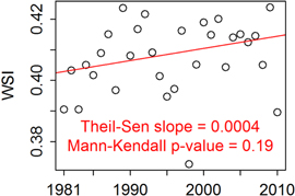
Schewe et al (2014) predicted increased water scarcity in the future, but also pointed to the large uncertainties. Our results indicate that global water scarcity increased from the period 1981–1990 to 2001–2010 (table 1). The Wilcoxon–Mann–Whitney test confirms that the monthly WSI considering total water resources is greater in the later than in the earlier decade (p-value = 0.0007). It is, however, only 53% likely that the increase in water scarcity actually took place. The Mann–Kendall trend test of global annual averages further highlights the large uncertainties involved, as the p-value of 0.19 indicates that there is no statistical evidence for a trend (figure 3) at the global scale.
Figure 3. 30-year trend of global annual average WSIs. Combination of Mann–Kendall trend test with Theil-Sen trend estimate.
Download figure:
Standard image High-resolution image
Some studies have found that dry regions are getting drier and wet regions are getting wetter (Liu and Allan 2013), although others have refuted such a phenomenon (Greve et al 2014). More relevant for human purposes are the trends in water scarcity. While we can confirm that water scarce regions are getting scarcer, we have to refute that water rich regions are getting richer. The Amazonian region is a counter-example, which is abundant in water, but is getting scarcer (figure 1). By contrast, Spain is scarce in water, but the scarcity is reducing because it is generally getting wetter even in some arid regions. That is why Greve et al (2014) disproved the dry getting drier paradigm. It is only 31% likely that global consumption-weighted water availability decreased and thereby intensified water scarcity. On the other hand, global water consumption is 59% probable to have risen and is therefore the major driver of increased water scarcity.
Similar to the paradigm on regional trends, Chou et al (2013) found that dry seasons are getting drier and wet seasons are getting wetter. As stated above, more relevant for human purposes are the trends in water scarcity. We investigated this seasonal trend for five major climate zones in the Northern hemisphere and three major climate zones in the Southern hemisphere excluding Antarctica (Peel et al 2007). Aside from the Northern polar climate zone, the scarce season is getting scarcer in all regions. By contrast, the abundant season is in no zones getting more abundant and monthly fluctuations of water scarcity are decreasing in most climate regions. Only in the Southern temperate climate zone, there is a 51% chance that water scarcity is fluctuating more (exhibits a larger standard deviation) in the later decade (2001–2010). However, extreme events such as prolonged droughts are not addressed by our monthly assessment.
Regional optimization versus crop choice
Water scarcity can be partly alleviated by technological improvements such as increased irrigation efficiency and desalination of seawater (Wada et al 2014a), but it requires a combination with soft path solutions (Gleick 2003). Two major soft pathways are (i) regional optimization (Ridoutt and Pfister 2010), which would require international trade agreements to be supplemented by regulations on water use sustainability (Vörösmarty et al 2015), and (ii) changes in diets (Jalava et al 2014). We therefore compared the CVs of blue water consumption among 160 countries and 147 food crops. The results indicated that the variability is higher for the same crop from different countries (CV higher for 8 out of 11 food groups) than among the global averages of different crops (CV higher for 3 out of 11 food groups), and therefore regional patterns are generally more important (table 2). However, this comparison was based on mass and is independent of the caloric or nutritional value which can be justified by consumers choosing amounts of food rather based on serving sizes than nutrient balances. While it can be effective to choose well which crops we eat and feed our farm animals, it is even more important to select the optimal location for the crop production. The greatest potential lies in regional optimization of the cultivation of cereals and roots and tubers.
Table 2. Coefficients of variations (CVs) for the same crop from different countries and for global averages of crops within the same crop group. For each group, the higher CV is presented in bold.
| Food group | Countries | Crops |
|---|---|---|
| Cereals | 1.58 | 0.34 |
| Forage | 1.11 | 0.58 |
| Fruits | 0.83 | 0.86 |
| Nuts | 0.68 | 0.90 |
| Oil-bearing crops | 1.08 | 0.92 |
| Pulses | 1.07 | 0.66 |
| Roots and tubers | 1.55 | 0.44 |
| Spices | 0.80 | 0.83 |
| Stimulants | 0.96 | 0.33 |
| Sugar crops | 0.92 | 0.18 |
| Vegetables | 0.81 | 0.78 |
The impacts of water consumption largely depend on the prevailing water scarcity, which together yield water scarcity footprints. Maize, rice and wheat are the three major staple food crops and as such provide a great opportunity to optimize humanity's water scarcity footprint of food. Their global production-weighted water scarcity footprints deviate significantly (p-values ≪ 0.05). Maize has the smallest footprint, followed by rice and finally wheat (table 3). The probabilities of one crop having a smaller footprint than the subsequent one are >60% on global average. Nonetheless, the location is also a crucial choice and offers further opportunities for optimization, as the major exporting countries always exhibit the largest footprint among the three countries investigated.
Table 3. Water scarcity footprint (WSF) for maize, rice and wheat per kilogram and per Mcal harvested crop for the three major exporting countries. A production-weighted global mean is also provided. The countries are sorted from high to low export volume. The country with the smallest WSF per Mcal out of the three major exporters is presented in bold.
| Product | Country | Consumption mean (l kg−1) | Consumption SD (l kg−1) | WSI mean | WSI SD | WSF (l kg−1) | WSF (l Mcal−1) | WSFa (l Mcal−1) |
|---|---|---|---|---|---|---|---|---|
| Maize | USA | 170 | 1.36 | 0.43 | 0.44 | 72 | 19.85 | 19.86 |
| Maize | Brazil | 37 | 2.63 | 0.21 | 0.32 | 8 | 2.10 | 2.10 |
| Maize | Argentina | 71 | 2.09 | 0.24 | 0.36 | 17 | 4.73 | 4.76 |
| Maize | Global | 178 | 1.36 | 0.37 | 0.41 | 65 | 17.90 | 17.90 |
| Rice | India | 447 | 1.29 | 0.67 | 0.28 | 297 | 82.13 | 82.14 |
| Rice | Vietnam | 37 | 1.50 | 0.27 | 0.29 | 10 | 2.75 | 2.75 |
| Rice | Thailand | 232 | 1.31 | 0.28 | 0.27 | 65 | 17.82 | 17.83 |
| Rice | Global | 239 | 1.26 | 0.42 | 0.40 | 101 | 27.81 | 27.81 |
| Wheat | USA | 379 | 1.55 | 0.43 | 0.44 | 161 | 47.64 | 47.65 |
| Wheat | Australia | 425 | 2.26 | 0.32 | 0.37 | 136 | 40.24 | 39.44 |
| Wheat | Canada | 66 | 3.21 | 0.06 | 0.12 | 4 | 1.15 | 1.20 |
| Wheat | Global | 385 | 1.29 | 0.39 | 0.41 | 150 | 44.29 | 44.29 |
aProbabilistic mean of 1000 Monte Carlo iterations derived from the geometric mean of water consumption and the arithmetic mean of WSI. The other WSF is deterministic.
Another example of a relevant crop choice is the selection of crops with similar functional ingredients such as caffeine in stimulant products. The global production-weighted water scarcity footprint of a standard cup of coffee amounts to 22 l/cup, while it amounts to 19 l/cup for tea (table 4). The Wilcoxon–Mann–Whitney test did not provide evidence of a significant difference in means for the two distributions (p-value = 0.3) and the probability that tea deprives other users of less water than coffee is only 50% globally. The WSF varies largely depending on the country of origin. Accounting for all the uncertainties in WSI and water consumption estimates, drinking a cup of tea from the major exporting country Sri Lanka (WSF of 7 l/cup) for a dose of 50 mg of caffeine is better in terms of water scarcity than drinking a cup of coffee from the major exporting country Vietnam (WSF of 15 l/cup) with a probability of 66%. By contrast, when drinking tea from China, the second largest tea exporter, it is 58% probable that it deprives other users of more water than when drinking coffee from Vietnam. Among the major coffee exporters (Vietnam, Brazil and Indonesia) Brazil causes the least water deprivation for the production of coffee and among the major tea exporters (Sri Lanka, China and Kenya) Kenya causes the least water deprivation for the production of tea.
Table 4. Water scarcity footprint (WSF) for coffee and tea per kilogram harvested crop and per cup of final product for the three major exporting countries. A production-weighted global mean is also provided. The countries are sorted from high to low export volume. The country with the smallest WSF per cup out of the three major exporters is presented in bold.
| Product | Country | Consumption mean (l kg−1) | Consumption SD (l kg−1) | WSI mean | WSI SD | WSF (l kg−1) | WSF (l/cup) | WSFa (l/cup) |
|---|---|---|---|---|---|---|---|---|
| Coffee | Vietnam | 1088 | 1.39 | 0.27 | 0.29 | 291 | 15.27 | 15.28 |
| Coffee | Brazil | 1104 | 2.19 | 0.21 | 0.32 | 231 | 12.16 | 12.28 |
| Coffee | Indonesia | 2109 | 1.29 | 0.59 | 0.41 | 1253 | 65.40 | 65.40 |
| Coffee | Global | 1618 | 1.65 | 0.25 | 0.34 | 409 | 21.40 | 21.53 |
| Tea | Sri Lanka | 865 | 1.68 | 0.64 | 0.33 | 552 | 6.88 | 6.73 |
| Tea | China | 4296 | 1.31 | 0.39 | 0.40 | 1677 | 20.38 | 20.38 |
| Tea | Kenya | 1285 | 2.11 | 0.11 | 0.17 | 138 | 1.90 | 1.75 |
| Tea | Global | 3660 | 1.34 | 0.43 | 0.40 | 1571 | 19.11 | 19.11 |
aProbabilistic mean of 1000 Monte Carlo iterations derived from the geometric mean of water consumption and the arithmetic mean of WSI. The other WSF is deterministic.
Personal budgets
Considering the global dimension of water scarcity, Hoekstra (2011) argues that institutional arrangements for water governance are needed. One possibility are water footprint quotas which encourage equitable sharing of our water resources and respect distributive fairness. We estimated personal budgets at 251 l d−1. Given that >85% of total consumption is used for agriculture (Döll and Siebert 2002, Shiklomanov and Rodda 2004), this leaves 35 l d−1 for domestic and industrial uses. This exceeds the minimal water requirements of 14 l d−1 needed for human health, social and economic development by a factor of 2.5—assuming 135 l d−1 withdrawals (Chenoweth 2008) and 10% consumptive use in these two sectors (Flörke et al 2013). As such, it should be feasible to restrict our current domestic and industrial consumption to the suggested personal budgets. The 216 l d−1 for agricultural water consumption remain the major challenge. The case study on stimulants reveals that one cup of coffee per day (∼85 l) may constitute ∼40% of the agricultural water budget and as such reduced consumption of these stimulants can considerably contribute to reduce the exceedance of our budgets, in addition to previously revealed potentials from diet change (Jalava et al 2014) and food waste reduction (Kummu et al 2012).
Conclusions
Water scarcity is and will continue to be a major global concern, which is demonstrated by a global consumption-weighted WSI of 0.51 in 2001 to 2010. The data suggest a slight increase in water scarcity over a 30-year period from 1981 to 2010; however, the trend is not statistically significant. Also the probability of an increase from the earlier to the later period is close to 50% and, as such, low. Independent of any trend, water scarcity is currently already so severe that strategies to alleviate water scarcity are urgently needed.
Reduction in irrigation is a major lever to reduce water scarcity. Regional optimization and crop choice both offer a high potential for that, but regional optimization has proven to be even more crucial. Information on the spatial distribution of water scarcity as provided in this study enables the identification of hotspots where sustainability measures are most needed and it points to regions that are more favourable for water consumption than alternative locations. The analysis carried out can identify improvement potentials in a global economy and might assist in political decisions about international trade regulations, but also in personal decisions with regards to crop choices. However, other environmental aspects such as land use impacts or climate change must be included for a more complete evaluation of suitable production.
Finally, models at the global level inherit large uncertainties which have to be communicated transparently to allow for proper decision-making. While many researchers fear that uncertainty might induce a loss in trust of stakeholders, its negligence might undermine science and lead to policy actions without sound scientific support. Uncertainty is inherent in any hydrological model, but also allows for covering a range of possible outcomes which makes it more likely for a prediction to turn out well (Beven 2006). Uncertainties are essential information when comparing two product variants such as crops, also from different countries, and we must therefore take care to quantify and communicate uncertainties in a way that is easily understandable to decision-makers. Percentage probabilities as derived in this study are a possible means of communication that is easy for non-experts to understand.
Acknowledgments
We thank Yoshihide Wada for providing a dataset on water withdrawals, Stefanie Hellweg for helpful comments on the manuscript and Christie Walker as well as Catherine Raptis for proofreading it.