

Abstract
Environmental justice (EJ) research has relied on ecological analyses of socio-demographic data from areal units to determine if particular populations are disproportionately burdened by toxic risks. This article advances quantitative EJ research by (a) examining whether statistical associations found for geographic units translate to relationships at the household level; (b) testing alternative explanations for distributional injustices never before investigated; and (c) applying a novel statistical technique appropriate for geographically-clustered data. Our study makes these advances by using generalized estimating equations to examine distributive environmental inequities in the Miami (Florida) metropolitan area, based on primary household-level survey data and census block-level cancer risk estimates of hazardous air pollutant (HAP) exposure from on-road mobile emission sources. In addition to modeling determinants of on-road HAP cancer risk among all survey participants, two subgroup models are estimated to examine whether determinants of risk differ based on disadvantaged minority (Hispanic and non-Hispanic Black) versus non-Hispanic white racial/ethnic status. Results reveal multiple determinants of risk exposure disparities. In the model including all survey participants, renter-occupancy, Hispanic and non-Hispanic black race/ethnicity, the desire to live close to work/urban services or public transportation, and higher risk perception are associated with greater on-road HAP cancer risk; the desire to live in an amenity-rich environment is associated with less risk. Divergent subgroup model results shed light on the previously unexamined role of racial/ethnic status in shaping determinants of risk exposures. While lower socioeconomic status and higher risk perception predict significantly greater on-road HAP cancer risk among disadvantaged minorities, the desire to live near work/urban services or public transport predict significantly greater risk among non-Hispanic whites. Findings have important implications for EJ research and practice in Miami and elsewhere.
Export citation and abstract BibTeX RIS

Content from this work may be used under the terms of the Creative Commons Attribution 3.0 licence. Any further distribution of this work must maintain attribution to the author(s) and the title of the work, journal citation and DOI.
1. Introduction
Distributional research on environmental justice (EJ) has depended almost exclusively on the use of aggregated census data from pre-defined geographic units at approximately the neighborhood level to determine if socially vulnerable populations are disproportionately burdened by toxic risks and hazards. Although results vary across quantitative EJ analyses, the bulk of studies conducted in the US and beyond indicate that racial/ethnic minority and lower socioeconomic status (SES) populations experience disproportionately high neighborhood-level exposures to toxic pollution risks (Mohai et al 2009a, Chakraborty et al 2011, Walker 2012). The reliance on ecologic study designs, however, has generally limited distributional EJ research in accounting for fine-scale individual- or household-level variation in relevant determinants and clarifying mechanisms that structure aggregate patterns. The role of household decision-making, for example, in patterning environmental injustices cannot be adequately examined when the traditional approach of analyzing aggregated population data across areal units is utilized.
This study addresses that key limitation and provides a new approach to EJ analysis based on a downscaled, household-level examination of determinants of residential exposure to cancer risks from transportation-generated HAPs in the Miami–Fort Lauderdale–West Palm Beach, Florida Metropolitan Statistical Area (USA), which includes Miami-Dade, Broward and Palm Beach Counties (hereafter 'Miami MSA'). It addresses two research questions. (1) Are cancer risks from HAP exposures distributed inequitably with respect to household-level factors of SES, housing tenure, race/ethnicity, risk perceptions, and residential decision-making considerations? (2) How do within-group distributional inequities in HAP exposures differ between disadvantaged minorities and non-Hispanic whites with respect to household-level factors identified in research question 1?
Our analysis makes three contributions to the literature on EJ analysis. First, because it is based on an examination of fine-scale, household-level primary data, it enables avoidance of the ecological fallacy, i.e., the assumption that findings based on analyses of aggregated socio-demographic data translate to relationships at the micro-level. Few published analyses have examined distributional EJ using household-level data (Mohai and Bryant 1992, 1998, Mohai et al 2009b, Crowder and Downey 2010, Collins et al 2015). Second, and related to the first, the data collected using our structured survey instrument enable examination of previously untested influences on distributional environmental inequities. These data are useful for assessing, for example, if a lack of awareness regarding air pollution health risks and/or particular residential decision-making priorities influence patterns of risk exposure, and, if so, whether those factors affect Hispanics and non-Hispanic blacks differently than non-Hispanic whites. This provides the basis for a novel, systematic evaluation of alternative explanations for fine-scale patterns of environmental injustice. Third, in order to statistically model patterns of environmental injustice, we employ generalized estimating equation (GEE) techniques, which adjust for geographic clustering and support population-averaged inferences about determinants of disproportionate exposure to HAPs. While GEEs have only been used in a few geographic analyses, our application demonstrates the utility of GEEs for addressing clustering in non-normally distributed data in order to support statistically valid inferences.
2. Study area: Miami MSA, Florida, USA
With a total population of 5.4 million, the Miami MSA is the largest metro area in Florida and the seventh largest in the US (figure 1). In terms of air pollution, the Miami MSA faces generally very high levels of ambient exposure to excess cancer risks from HAPs; the three counties of the Miami MSA are in the highest decile of HAP cancer risk among all Florida counties (USEPA (US Environmental Protection Agency) (2011a)). The Miami MSA is composed of a highly segregated, socially diverse population with high proportions of residents from racial/ethnic minority backgrounds. Hispanics comprise 41.6% of the total population, followed by non-Hispanic whites (34.8%) and non-Hispanic blacks (19.7%). Surprisingly little distributive EJ research has been conducted in the Miami MSA. To our knowledge, Grineski et al (2013) provide the only distributional EJ study focused on vehicular air pollution conducted in the Miami MSA; their results indicate a pattern of environmental injustice that generally corresponds with findings from many other studies. Employing spatial regression models that account for spatial dependence in the data at the census tract level, they found a positive and significant association for the percentage of the tract population that was Hispanic—and a negative and significant association for median household income—with on-road cancer risks from HAPs (Grineski et al 2013). Whether similar relationships exist at the household level is unknown.
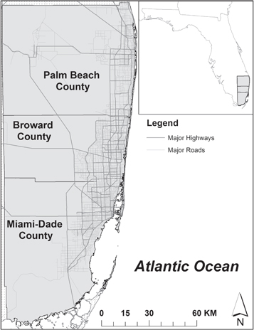
Figure 1. Location of the Miami MSA, Florida, USA study area.
Download figure:
Standard image High-resolution image3. Methods
3.1. Structured survey
Data used to construct explanatory variables are derived from an Institutional Review Board-approved cross-sectional telephone survey of randomly selected adults in the Miami MSA. Surveys lasted 30 min on average and were administered by trained bilingual Spanish–English interviewers; a US$10 cash incentive was offered to each survey respondent. Details regarding the structured survey sampling strategy are provided in Collins et al (2015).
To obtain a socially and spatially representative sample, we employed a two-stage sampling approach (figure 2). It involved first stratifying and randomly selecting a subset of census tracts (based on 2010 US decennial census boundaries) across geographic quadrants (containing equal number of tracts) of the Miami MSA in stage 1, and then completing telephone interviews with five randomly selected residents in each selected census tract in stage 2. A US census tract is a relatively small geographic unit, typically with a population size between 1200 and 8000 people. To select the census tracts for stage 1, within each quadrant, census tracts were stratified into quintiles based on a measure created through factor analysis of two US census data-derived variables. The two variables represent the race/ethnicity and SES constructs that are integral to EJ research: (i) percent of the census tract population that is non-Hispanic white, and (ii) median household income of the census tract. The Cronbach's alpha of 0.608 for the two-variable factor indicates adequate reliability. Within each quintile (stratified based on that factor) in each quadrant, we randomly selected six census tracts, for a total of 30 selected census tracts per quadrant. Figure 3 displays the resulting random stratified sample of census tracts. Stage 2 called for completing telephone interviews with five randomly selected householders in each of 120 randomly selected census tracts in the Miami MSA, for a total of 600 surveys. We were able to exceed our target by culling data from an additional 50 surveys participants in the Miami MSA.
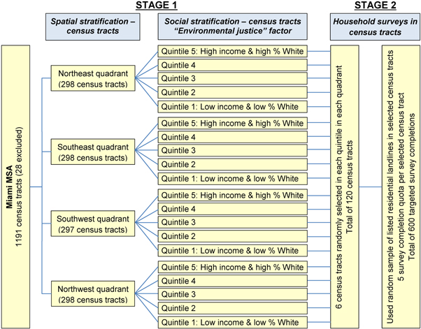
Figure 2. Two-stage sampling approach.
Download figure:
Standard image High-resolution image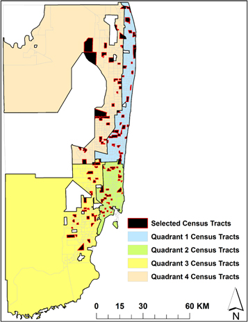
Figure 3. Census tract sample (stage 1), Miami MSA.
Download figure:
Standard image High-resolution imageThe survey was administered from 28 June to 1 August, 2012. Each household survey was completed with one adult who identified as being engaged in decision-making on behalf of the household (i.e., a householder). Overall, the survey had a response rate of 33%, which is comparable to that achieved in recent published studies based on random digit dialing surveys (e.g., Mumpower et al 2013). This response rate is for the total sample (n = 1,237), which included participants from both metropolitan Houston (Texas) and the Miami MSA; the same sampling strategy was applied in metro Houston (see Collins et al 2015). Studies indicate that similar and even substantially lower survey response rates can yield representative samples (Visser et al 1996, Curtin et al 2000, Keeter et al 2006, Holbrook et al 2007), and a meta-analysis found response rates to poorly predict nonresponse bias (Groves and Peytcheva 2008). Our sampling design yielded a generally representative sample. For example, compared to 2010 US Decennial Census estimates for the Miami MSA, our sample is generally representative in terms of percentages of adult Hispanics (34 versus 41%) and adult blacks (16 versus 18%). Participants were placed at their residential locations using address-based geocoding with ArcGIS 10 and Google Earth.
We analyzed data for 610 participants for whom home address data were geocodable and nearly complete survey data were available; 40 were excluded due to excessive data missingness for the analysis variables. In terms of participants' demographic characteristics, 48% are non-Hispanic white, 32% are Hispanic, and 14% are non-Hispanic black. Median total annual household income (2011) is $35 000 (mean = $53 551). The average age of the participating householder is 62 years, and the range is 18–94 (as only adults were allowed to participate). Participants are 63% female and 37% male.
3.2. Dependent variable: on-road mobile HAP cancer risk
Our dependent variable is estimated lifetime cancer risk from inhalation exposure to HAPs faced by each participating household from on-road mobile emission sources for the census block within which each household resided at the time of the survey. Data were derived from the US Environmental Protection Agency's (EPA) National-Scale Air Toxics Assessment (NATA), which has emerged in recent years as a standard data source for distributive EJ analysis in the US (Chakraborty 2009, Grineski and Collins 2010, Collins et al 2011, Chakraborty et al 2014, Grineski et al 2015). HAPs, also known as air toxics or non-criteria air pollutants, include 188 specific substances identified by the Clean Air Act Amendments of 1990 that are known to cause or suspected of causing cancer and other serious health problems. Our study utilizes the 2005 NATA dataset, which was released in 2011 and is the most recent available. The 2005 dataset does not provide a perfect temporal fit with the survey data (from 2012), but it is the best available match. The dependent variable includes chronic cancer risks associated with inhalation exposure to HAPs released by on-road mobile sources. For this analysis, we selected only the on-road mobile category because it comprises the largest source (54%) of cancer risk from local, known HAP emission sources in the Miami MSA. Our analysis of data on cancer risks from on-road emission sources represents an advance upon the US EPA Toxics Release Inventory (TRI) data used in two published household-level EJ studies (Mohai et al 2009b, Crowder and Downey 2010); TRI data are inadequate to assess health risks associated with HAP exposures, particularly in contexts such as the Miami MSA where on-road emissions are the primary source of HAP exposures. On-road mobile sources include motorized vehicles operating on roads and highways (e.g., cars, trucks, busses). Currently, NATA is the best secondary data source for spatially explicit characterization of air toxics risk exposure in US metro areas (McCarthy et al 2009, Marshall et al 2014).
The methods used to generate cancer risk estimates are well documented (USEPA 2011b, 2013). Although the NATA quantifies cancer risks in terms of lifetime exposure, they provide estimates of current cancer risks associated with HAP exposures from on-road emission sources at the census block level. To create the dependent variable, the home location of each respondent was geocoded and assigned the NATA on-road cancer risk score for the census block within which they were located. The block level estimates that we use in this study were acquired directly from the USEPA and are at a finer spatial resolution than the publically available census tract estimates that have been used to assign risk values to people's home addresses in other studies (Lupo et al 2011, Roberts et al 2013).
3.3. Explanatory variables
Explanatory variables were selected to test alternative theoretical explanations for inequitable exposure to HAPs; they specifically represent the domains of race/ethnicity, SES, housing tenure, risk perception, and residential locational decision-making. The race/ethnicity, SES, and housing tenure measures used here have long been central to EJ research. The risk perception and residential locational decision-making variables have not traditionally been examined by quantitative EJ scholars, largely due to the reliance on aggregated secondary datasets lacking information on such domains. Each measure was developed from data collected via the household survey.
Race/ethnicity is analyzed with three variables representing the self-identification of householders who responded to the survey: Hispanic/Latino ('Hispanic'), non-Hispanic black ('Black'), and non-Hispanic 'Other minority'; non-Hispanic whites comprise the reference group. 'SES' is analyzed as a two-item factor (Cronbach's alpha = 0.633) that includes (i) years of education of the household member with highest educational attainment and (ii) total household income for 2011. Housing tenure is measured using renter-occupant status ('Renter'), which reflects greater housing instability, as well as less political engagement and access to resources (Pastor et al 2005). Air pollution health risk perception ('Risk perception') is analyzed based on participating householders' levels of concern about the possibility of air pollution causing health problems for themselves or members of their households (Bickerstaff 2004, Bickerstaff and Walker 2001). The sex of the participating householder is included as a control variable, since the amplification of risk perception among females compared to males is well-documented (Gustafson 1998). Mobility and residential locational decision-making are receiving renewed attention in the EJ literature (Taylor 2014, Collins et al 2015, Hernandez et al 2015). Residential locational decision-making is examined here with four variables representing the degree to which participating householders were influenced in moving to their current home sites by specific considerations (Collins 2008, 2009). These include: being close to 'Work/urban services' (four-item factor, Cronbach's alpha = 0.698), 'Public transport' (only one item), 'Cultural attractors' (five-item factor, Cronbach's alpha = 0.802), and 'Environmental exclusivity' (seven-item factor, Cronbach's alpha = 0.728). The specific items included in each factor are listed in table 1. Except for the dichotomous variables (Hispanic, Black, Other minority, and Renter), all explanatory variables were standardized/centered before entry in the statistical models and analyzed as continuous measures. See table 1 for descriptions of the variables before standardization.
Table 1. Analysis variables: Source, metric, and descriptive statistics (n = 610)a.
| Variable | Source | Metric | Meanb | St. Dev. | Min.–Max. | % Missing |
|---|---|---|---|---|---|---|
| On-road mobile hazardous air pollutant cancer risk | USEPA 2005 National Air Toxics Assessment, census block level | Total excess cancer risk from HAPs (persons per million) from on-road mobile emission sources | 8.35 | 4.30 | 0.97–23.43 | 0.0 |
| Hispanic | Surveyc: are you of Hispanic, Latino, or Spanish origin? | 0 = No | 0.316 | 0–1 | 1.8 | |
| 1 = Yes | ||||||
| Black | Surveyc: which of the following best describes your race? .... Black/African American | 0 = No | 0.135 | 0–1 | 1.5 | |
| 1 = Yes | ||||||
| Other minority | Surveyc: which of the following best describes your race? | 0 = No to all | 0.059 | 0–1 | 2.2 | |
| American Indian or Alaskan Native; Asian; Pacific Islander; some other (non-white) race | 1 = Yes to any | |||||
| SES (two-item factor) | Factor | 0.004 | 0.997 | −2.97–2.14 | 26.4 | |
| Surveyc: | ||||||
| (i) What was your total household income for the year 2011 before taxes? | 1 = <$10 000–10 = >$249 999 | 53 551 | 54 869 | <$10–≥$250 K | 25.6 | |
| (ii) Thinking about the person in your household with the highest educational degree received or level of school completed—what is the highest grade or level of school that this person has completed? | 0 = No formal schooling—21 = PhD degree | 15.05 | 3.260 | 0–21 | 1.1 | |
| Renter | Surveyc: is this home rented? | 0 = No | 0.229 | 0–1 | 3.4 | |
| 1 = Yes | ||||||
| Risk perception | Survey: how concerned are you about the possibility of air pollution causing health problems to you or members of your household? | 1 = Not concerned—5 = extremely concerned | 3.018 | 1.394 | 1–5 | 0.5 |
| Work/urban services (four-item factor) | Factor | 1 = Not a consideration—5 = a very important consideration | 0.015 | 0.989 | −2.24–1.48 | 2.3 |
| Surveyd: Close to | ||||||
| (i) ...work or jobs | 3.168 | 1.584 | 1–5 | 1.5 | ||
| (ii) ...school, college, or university | 3.002 | 1.649 | 1–5 | 0.5 | ||
| (iii) ...a medical clinic or hospital | 3.675 | 1.346 | 1–5 | 0.0 | ||
| (iv) ...shopping | 3.704 | 1.339 | 1–5 | 0.3 | ||
| Public transport | Surveyd: close to a bus route or access to public transportation | 1 = Not a consideration—5 = a very important consideration | 2.923 | 1.680 | 1–5 | 0.5 |
| Cultural attractors (five-item factor) | Factor | 1 = Not a consideration—5 = a very important consideration | 0.000 | 1.000 | −1.93−1.49 | 1.0 |
| Surveyd: close to... | ||||||
| (i) ...family or friends | 3.289 | 1.568 | 1–5 | 0.0 | ||
| (ii) ...people who speak your language | 3.569 | 1.541 | 1–5 | 0.0 | ||
| (iii) ...restaurants that serve food you prefer—for example, food from your homeland or food that you grew up eating | 3.197 | 1.489 | 1–5 | 0.0 | ||
| (iv) ...your church | 3.120 | 1.588 | 1–5 | 0.7 | ||
| (v) ...places where members of your household can interact with people from your cultural background | 3.175 | 1.501 | 1–5 | 0.5 | ||
| Environmental amenities (seven-item factor) | Factor | 1 = Not a consideration—5 = a very important consideration | 0.014 | 0.991 | −2.21–2.08 | 3.8 |
| Surveyd: | ||||||
| (i) good views from home | 3.341 | 1.564 | 1–5 | 1.0 | ||
| (ii) waterfront or beachfront property | 2.220 | 1.659 | 1–5 | 1.0 | ||
| (iii) home and property were visually attractive | 3.765 | 1.366 | 1–5 | 0.8 | ||
| (iv) privacy or seclusion | 3.558 | 1.364 | 1–5 | 0.7 | ||
| (v) exclusive neighborhood | 3.097 | 1.478 | 1–5 | 0.3 | ||
| (vi) close to the coast or beach | 2.910 | 1.497 | 1–5 | 0.3 | ||
| (vii) close to a golf course | 2.295 | 1.594 | 1–5 | 0.5 |
aDescriptive statistics are reported for original data prior to multiple imputation. bRepresents the proportion coded as '1' for the dichotomous variables (Hispanic, Black, Other minority, and Renter). cAdapted from the 2011 American Community Survey instrument. dThe residential locational decision-making items (Work/urban services, Public transport, Cultural attractors, and Environmental amenities) were prefaced by interviewers with this statement: 'The following questions ask about why you and your household decided to live at your current place of residence in the Miami Metro Area. What level of consideration was given to the following features when you constructed, purchased or rented your current home? Please respond with a number on a scale ranging from 1 to 5, with 1 meaning a feature was 'Not a consideration at all' and 5 meaning a feature was 'A very important consideration'. It is important that you respond by indicating the level of consideration your household gave to each feature rather than by indicating whether your current home does or does not have each feature. For example, please indicate a feature was '5—A very important consideration' if that feature was a very important reason why you decided to live in your current home. Please do not indicate a feature was 'A very important consideration' only because your home happens to have that feature'.
3.4. Analysis approach
Multiple imputation (MI) was employed to address nonresponse bias associated with missing values for all analysis variables derived from the household survey. MI is a best practice for addressing missing data in statistical analysis (Baraldi and Enders 2010, McPherson et al 2012, Van Buuren 2012). MI involves creating multiple sets of values for missing observations using a regression-based approach. It is used to avoid the bias that can occur when missing values are not missing completely at random (Penn 2007) and is appropriate for self-reported survey data (Enders 2010). Using SPSS (version 20 software), 20 imputed datasets were specified to increase power and 200 between-imputation iterations were used to ensure that the resulting imputations were independent of each other (Enders 2010). In order to generate results that we report for the GEEs, SPSS was used to run the statistics 20 times (once per imputed dataset) and then pool the results.
GEEs with robust (i.e., Huber/White) covariance estimates extend the generalized linear model of Nelder and Wedderburn (1972) to accommodate clustered data. GEEs are widely used for analyses of clustered data in the biological and epidemiological sciences (Liang and Zeger 1986, Zeger and Liang 1986, Diggle et al 1994), but have been scarcely employed in human geographic analyses (see Neumayer 2004, Mobley et al 2012, Root 2012, and Collins et al 2015 for exceptions). They provide a general method for the analyses of clustered variables, and relax several assumptions of traditional regression models. GEEs enable us to test alternative theoretical explanations for environmental inequalities in reference to a non-normally distributed dependent variable, while accounting for geographic clustering. For our purposes, GEEs are preferable to other modeling approaches that account for non-independence of data (e.g. multilevel models) since they estimate unbiased population-averaged (i.e., marginal) regression coefficients, even with misspecification of the correlation structure when using a robust variance estimator (Liang and Zeger 1986, Zeger and Liang 1986), which is appropriate for analyses of general patterns of environmental inequality across subpopulations. Additionally, because our focus is on population-averaged determinants of HAP cancer risk exposure at the household level, not neighborhood effects, GEEs are appropriate because the intracluster correlation estimates are adjusted for as nuisance parameters and not modeled (as in multilevel modeling approaches) (Diez Roux 2002).
To fit a GEE, clusters of observations must be defined. It is assumed that observations from within a cluster are correlated, while observations from different clusters are independent. Following Collins et al (2015), GEEs with clusters defined based on median decade of housing construction by geographic quadrant for census tracts in which surveyed households reside were used in the final models presented here in order to adjust for spatial clustering. Geographic quadrants correspond with those used to implement the two-stage cluster sampling design (figure 3). Eight median year of housing construction categories correspond with the response options for an American Community Survey instrument 'Housing' item ('About when was this building first built?'): '2000 or later', '1990–1999', '1980–1989', '1970–1979', '1960–1969', '1950–1959', '1940–1949', and '1939 or earlier' (US Bureau of the Census 2011). This cluster definition method was selected over other alternatives (e.g., defining clusters based census tract of residence) since GEE techniques assume dependence of observations within clusters and independence between clusters. These assumptions would be untenable if only census tract IDs were used to define clusters, since data for households living in separate census tracts—but within the same urban developmental context with shared socio-demographic characteristics—would be treated as independent. The median year of home construction by geographic quadrant method of cluster definition used here much more closely corresponds with the urban developmental context within which households are nested. Using these two variables to define clusters is also theoretically informed, since they correspond with spatial and temporal contextual built-environmental features associated with the historical-geographical formation of environmental inequality (Boone and Modarres 1999, Pulido 2000, Bolin et al 2005).
GEEs also require the specification of an intracluster dependency correlation matrix, known as the working correlation matrix (Liang and Zeger 1986, Zeger and Liang 1986). While robust estimation may yield correct standard errors even if the working correlation matrix has been misspecified, correct specification of the correlation structure enhances efficiency (Wang and Carey 2003). Selecting among several specifications should be guided by substantive reasons when possible, and sensitivity analyses of different specifications of the intra cluster correlation matrix are advised (Zorn 2001, Wang and Carey 2003). For this analysis, two correlation structure specifications available in SPSS were substantive candidates: (1) independent, which assumes the nonexistence of dependency (more-or-less a null-model for clustering); and (2) exchangeable, which assumes constant intracluster dependency (i.e., compound symmetry), so that all the off-diagonal elements of the correlation matrix are equal. We conducted sensitivity analyses by running all GEEs with both independent and exchangeable working correlation matrices, using quasi-likelihood under independence criterion (QIC) goodness-of-fit coefficients to determine the best working correlation specification (Garson 2012). For all models, QIC tests indicated that the exchangeable specification performed better than the independent. Thus, results for models with the exchangeable specification only are presented here.
GEEs imply no strict distribution assumptions for independent variables and are appropriate for use with non-normally distributed outcome variables, which is the case here. A gamma distribution with a logarithmic link function was specified for each GEE, because the dependent variable is comprised of positive scale values skewed toward larger positive values. The two explanatory variables based on ordinal measures (risk perception and public transport) are analyzed as continuous predictors in each GEE model. This approach is considered a best practice in MI when imputing missing data and estimating model parameters, since rounding off imputed values based on discrete categorical specifications has been shown to produce more biased parameter estimates in analysis models (Horton et al 2003, Allison 2005, Enders 2010, Rodwell et al 2014).
To address research question 1, we began by estimating a GEE model to examine the effects of the explanatory variables on the dependent variable, cancer risk from on-road HAPs, using data for all survey participants. Next, to address research question 2, we estimated two subgroup models to examine whether determinants of on-road HAP cancer risk exposures differ between Hispanic and non-Hispanic black versus non-Hispanic white survey participants. Since the sample size of 86 non-Hispanic black survey participants is too small (based on a power analysis) to support a separate subgroup analysis, we combined the Hispanic-Latino/a and non-Hispanic black samples into one disadvantaged minority subgroup. We made that decision for two reasons. One, these are the two racial/ethnic groups well-represented in our sample with a shared social status of having been marginalized/disadvantaged in the US context. Two, a preliminary sensitivity analysis of separate Hispanic and non-Hispanic black subgroup GEE models indicated that the directionality and significance of associations between the explanatory variables and exposures to on-road HAP cancer risks were similar between the two groups, and also in alignment with GEE results from the combined Black-Hispanic subgroup model reported here. According to our diagnostic tests (variance inflation factor, tolerance, and condition index criteria (Belsley et al 1980)), inferences from the GEEs were not affected by multicollinearity problems.
4. Results
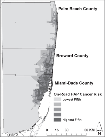
The spatial distribution of exposure to HAP cancer risk from on-road mobile sources in the Miami MSA is depicted in figure 4. Blocks facing the highest risks are concentrated in the central city areas and linearly along the main transportation corridors. Among all survey participants, the mean total estimated cancer risks from on-road HAP exposures at home sites was 8.4 excess deaths (per one million people) (see table 1). While not reported in table 1, the mean on-road HAP cancer risks of Hispanic and Black participants are 10.1 and 10.0 excess deaths (per million persons), respectively, both of which are well above the mean value of 7.1 for non-Hispanic whites.
Figure 4. Distribution of hazardous air pollutant cancer risk from on-road mobile sources by census block, Miami MSA.
Download figure:
Standard image High-resolution image
Table 2 presents pooled GEE results for Model 1, which predicts home site HAP cancer risk from on-road sources among all Miami MSA survey participants. Results show that being a Renter, Hispanic or Black, having the locational decision consideration of living near Work/urban services or Public transportation, and Risk perception are positively and statistically significantly associated with greater on-road HAP cancer risk at the p < 0.05 level. Placing more emphasis on environmental amenities in the residential locational decision-making process is significantly associated with less on-road HAP cancer risk.
Table 2. Results from a generalized estimating equations predicting hazardous air pollutant cancer risk from on-road mobile sources for (A) all cases, (B) Hispanics and Blacks, and (C) non-Hispanic whites.
| (A) Model 1: all cases (n = 610)a | (B) Model 2: Hispanics and Blacks (n = 279)b | (C) Model 3: non-Hispanic whites (n = 296)c | |||||||
|---|---|---|---|---|---|---|---|---|---|
| Variable | Beta | SE | 95% CI | Beta | SE | 95% CI | Beta | SE | 95% CI |
| (Intercept) | 2.112 | 0.091 | (1.935, 2.290)*** | 2.224 | 0.096 | (2.036, 2.412)*** | 2.086 | 0.100 | (1.890, 2.281)*** |
| SES | −0.012 | 0.018 | (−0.047, 0.023) | −0.041 | 0.016 | (−0.072, −0.009)** | 0.005 | 0.025 | (−0.044, 0.054) |
| Renter | 0.090 | 0.038 | (0.015, 0.165)** | 0.051 | 0.068 | (−0.082, 0.185) | 0.125 | 0.076 | (−0.024, 0.274) |
| Hispanic | 0.097 | 0.030 | (0.039, 0.156)*** | — | — | — | — | — | — |
| Black | 0.129 | 0.063 | (0.007, 0.252)** | — | — | — | — | — | — |
| Other minority | −0.061 | 0.061 | (−0.180, 0.059) | — | — | — | — | — | — |
| Work/urban services | 0.050 | 0.021 | (0.009, 0.090)** | 0.012 | 0.029 | (−0.044, 0.069) | 0.085 | 0.030 | (0.026, 0.145)*** |
| Public transport | 0.038 | 0.019 | (0.000, 0.075)** | 0.026 | 0.029 | (−0.030, 0.082) | 0.063 | 0.022 | (0.020, 0.106)*** |
| Cultural attractors | −0.025 | 0.017 | (−0.058, 0.008) | 0.002 | 0.025 | (−0.048, 0.052) | −0.038 | 0.036 | (−0.107, 0.032) |
| Environmental amenities | −0.036 | 0.016 | (−0.068, −0.005)** | −0.039 | 0.030 | (−0.097, 0.020) | −0.046 | 0.033 | (−0.110, 0.018) |
| Risk perception | 0.025 | 0.012 | (0.002, 0.048)** | 0.034 | 0.016 | (0.003, 0.065)** | 0.001 | 0.017 | (−0.032, 0.033) |
| (Scale) | 0.208 | 0.001 | 0.215 | 0.003 | 0.203 | 0.003 | |||
*p < 0.1; **p < 0.05; ***p < 0.01. aExchangeable correlation matrix; number of clusters = 20; number of measurements per cluster = 3 (min) to 60 (max). Correlation matrix dimension = 610. Model fit: range of QIC values for multiply imputed datasets = 207.266–210.157 (original data=95.255). Participant sex is included as a control and has a statistically non-significant relationship with hazardous air pollutant cancer risk. bExchangeable correlation matrix; number of clusters = 19; number of measurements per cluster = 1 (min) to 44 (max). Correlation matrix dimension = 278. Model fit: range of QIC values for multiply imputed datasets = 90.209–94.759 (original data = 47.789). Participant sex is included as a control and has a statistically non-significant relationship with hazardous air pollutant cancer risk. cExchangeable correlation matrix; number of clusters = 18; number of measurements per cluster = 1 (min) to 42 (max). Correlation matrix dimension = 296. Model fit: range of QIC values for multiply imputed datasets = 102.388–107.985 (original data = 47.178). Participant sex is included as a control and has a statistically non-significant relationship with hazardous air pollutant cancer risk.
Table 2 presents GEE results for Model 2, which includes data for households in the Hispanic and Black subgroup to predict home site HAP cancer risk from on-road sources. Results show that—among Hispanic and Black participants—lower SES and greater Risk perception are statistically significantly associated with increased on-road HAP cancer risk. Table 2 also presents GEE results for Model 3, which includes data for 296 households in the non-Hispanic white subgroup to predict home site HAP cancer risk from on-road sources. Results show that having the locational decision considerations of living near Work/urban services or Public transit are positively associated with on-road HAP cancer risk among non-Hispanic white participants.
5. Discussion
To summarize the findings, in terms of research question 1 (Model 1), renter-occupancy, Hispanic status, Black status, the desire to live close to work/services or public transit, and higher risk perception are all associated with greater on-road HAP cancer risk, while the desire to live in an exclusive, amenity-rich environment is associated with less risk. In terms of their significance and direction, most traditional EJ variables (Renter, Hispanic, Black) emerged as robust influences on patterns of exposure to HAPs from on-road sources at the household level. Those study results provide support at the household-level for arguments that EJ scholars have made based on neighborhood-level secondary data analyses for more than two decades. However, by examining variables related to residents' locational decision-making and risk perceptions, we were able to test the relative importance of alternative hypotheses regarding social influences on disproportionate patterns of risk exposure. In our analysis, residential locational decision-making factors—including the imperative of living close to work/services and public transit—emerged as important determinants of risk exposures. Risk perception also contributed substantial explanatory power, based on a comparison of model fit statistics between Model 1 and a model excluding the risk perception variable (results not shown). These results provide strong empirical support for the need to more carefully consider the roles of residential locational decision-making and risk perception in distributional EJ research.
Our household-level results from Model 1 (all participants) provide some novel and disturbing insights into compositional processes that articulate with structured inequalities in the (re) production environmental injustice. Those who are at greatest air pollution risk tend to have an awareness of their heightened exposure. Unfortunately, it appears that finding a home with access to public transportation channels some residents toward riskier residential locations; to compound this injustice, vehicular HAP exposure risks for public transport-reliant individuals are in all likelihood amplified through repeated, long-term roadside exposures. In sum, individuals reliant on public transportation reap the fewest benefits from the private automobile-based transit system in Miami, yet they also bear great costs. This reflects how compounding disadvantages may reinforce patterns of environmental injustice. On the other hand, the pursuit of a home in an exclusive residential setting with environmental amenities comes with the added benefit of reduced on-road HAP cancer risks. This reflects how environmental privilege—in tandem with disadvantage—may mutually reinforce environmentally unjust structures.
In terms of research question 2, results diverge between the Hispanic and Black versus non-Hispanic white subgroups, which indicates that determinants of on-road HAP cancer risk exposures vary by race/ethnicity. Note that the Hispanic and Black variables have the largest beta coefficients in Model 1 (including all cases), which indicates that they are the best predictors of residential exposure to on-road HAP cancer risks. The subgroup analysis results (Models 2 and 3) show that lower SES and higher risk perception predict significantly greater HAP risk among Hispanics and Blacks, but not among non-Hispanic whites. This suggests that disproportionate risks experienced by Hispanics and Blacks are not attributable to dampened risk perceptions or the desire to live close to work/urban services, which are critiques that have been leveled by some academic skeptics of EJ activists' claims. Instead, results indicate that residents—and disadvantaged minorities in particular—are to some degree well aware of the air pollution health risks they face. The subgroup analysis results suggest that—among Hispanics and Blacks—the most important influences on household-level patterns of exposure to cancer risks from on-road HAPs reflect mutually reinforcing disadvantages associated with low SES, and, by extension, processes of socio-environmental marginalization. Disproportionate risks appear to be driven primarily by structured racial/ethnic and socioeconomic disadvantages in the context of Miami, not by lack of awareness on the part of lower income minority people, nor by the strong pull of locational benefits—such as work opportunities or cultural attractors—that may be spatially associated with sources of air pollution. On the other hand, subgroup model results paint a more complex picture of determinants of on-road HAP risk for non-Hispanic whites, in that their disproportionate within-group exposures are less directly attributable to socioeconomic marginality and more directly to locational decision-making considerations. Among non-Hispanic whites, the desire to live near work/urban services or public transport predict significantly greater on-road HAP risk. This suggests that increased HAP risk exposures among non-Hispanic whites are driven more powerfully by their relatively wider range of residential choice (in comparison to Hispanics and Blacks) as they pursue living arrangements within the constraints of a highly unequal metropolis. In sum, low SES is the most important determinant of residential exposures to on-road HAP cancer risks among disadvantaged minorities, while preferences for living near work/urban services and public transit are the most important determinants for non-Hispanic whites. Black and Hispanic people do not appear to have the range of residential locational choice based on neighborhood amenities that is available to whites. Thus, subgroup model results appear to support the argument that housing discrimination and segregation may limit the options of racial/ethnic minorities in a manner that amplifies their exposures to on-road HAP cancer risks, and that minorities of lower SES are especially vulnerable.
There are several caveats associated with the methodology and data used for this study. Although the census block level cancer risk estimates we obtained from the USEPA's 2005 NATA provide more locational precision than has been achieved in previous studies employing NATA data, there are specific limitations associated with relying on this dataset as a source for our dependent variable. First, the NATA includes risks from only direct inhalation of the emitted air toxics and excludes exposure from other pathways such as ingestion or skin contact. Second, the NATA risk estimates only include individual and additive health effects; synergistic interactions among pollutants may pose additional cancer risks that are not examined in this study. Third, the assessment does not include exposure to vehicular HAPs produced indoors, such as evaporative benzene emissions from cars in attached garages. Fourth, the NATA risk estimates do not consider the length of residence of the surveyed households at their current home addresses. Finally, there is a seven-year gap between the 2005 NATA data used to formulate the dependent variable and the 2012 survey data used to create the independent variables. Following previous EJ studies that utilized NATA data, we assumed that relative levels of exposure to HAP cancer risks at the block level across the Miami MSA have remained constant between 2005 and 2012. This assumption is supported by the fact the spatial distribution of major surface streets, freeways, and other on-road sources of emissions in the Miami MSA has changed very little across that seven-year time gap.
6. Conclusions
In sum, this study makes substantial contributions to quantitative EJ research that are relevant to research and practice in US as well as international contexts. Findings demonstrate that some but not all statistical associations found for geographic units based on a conventional quantitative EJ analysis translate to relationships at the household level. For example, the tract-level association observed for Hispanic status with greater on-road HAP cancer risk by Grineski et al (2013) for the Miami MSA was also found here at the household level. However, the significant association between Black status and greater on-road HAP cancer risk found here was not observed by Grineski et al (2013). Additionally, our study demonstrates the utility of the GEE approach for EJ analysts grappling with geographically-clustered and non-normally distributed data.
More importantly, our focus on previously unexamined, alternative explanations for distributional injustices indicates that patterns of environmental inequity are attributable to multiple causes, some of which have received scant attention in EJ research and policy formulation. For example, the influence of structured disadvantages on household-level decision-making revealed by our analysis suggests that narrowly-conceived approaches which stovepipe EJ principles into specific environmental decision-making domains (e.g., regarding locational decisions for new industrial facilities or freeways) will not adequately address the injustices embedded in residential locational decision-making processes (that generate unequal exposures to hazards and access to amenities). Thus, broadly-conceived state interventions that provide more just structures for household decision-making are needed.
This study illustrates the utility of micro-level compositional EJ research for comprehensively examining patterns of environmental injustice and revealing alternative mechanisms that have been overlooked by ecological EJ studies. Future micro-level distributive EJ research should seek to employ mixed methods approaches focused on people's decision-making regarding costs and benefits associated with high-risk residential locations, including their subjectivities and differential material constraints, in order to better characterize and eventually address the environmental injustices they experience. While our study makes an important contribution to EJ analysis through the consideration of household-level information, similar research throughout the world is needed to develop a more complete understanding of distributive environmental injustices. In particular, comparative international research is needed to examine the influence of household-level factors (such as SES and locational decision-making) on risk exposures in contexts where the state intervenes more and less directly in the promotion of social equity.
Acknowledgments
We acknowledge US National Science Foundation (NSF) grants CMMI-1129984 and CMMI-1536113 for funding this work, and Marilyn Montgomery for her assistance with database preparation. The content is solely the responsibility of the authors and does not necessarily reflect the views of the USNSF.