

Abstract
The energy consumption of worm robots is composed of three parts: heat losses in the motors, internal friction losses of the worm device and mechanical energy locomotion requirements which we refer to as the cost of transport (COT). The COT, which is the main focus of this paper, is composed of work against two types of external factors: (i) the resisting forces, such as weight, tether force, or fluid drag for robots navigating inside wet environments and (ii) sliding friction forces that may result from sliding either forward or backward. In a previous work, we determined the mechanical energy requirement of worm robot locomotion over compliant surfaces, independently of the efficiency of the worm device. Analytical results were obtained by summing up the external work done on the robot and alternatively, by integrating the actuator forces over the actuator motions. In this paper, we present experimental results for an earthworm robot fitted with compliant contacts and these are post-processed to estimate the energy expenditure of the device. The results show that due to compliance, the COT of our device is increased by up to four-fold compared to theoretical predictions for rigid-contact worm-like locomotion.
Export citation and abstract BibTeX RIS
1. Introduction
Recent attempts at designing untethered worm robots, for locomotion inside pipes for maintenance tasks, or inside biological vessels for medical applications, highlighted the need for energy efficient devices for prolonged usage and longer travel distances. Over the past decades, several research groups designed and constructed small robots for in-pipe inspection (Hayashi and Iwatsuki 1998, Buertetto and Ruggiu 2001, Arena et al 2006, Lim et al 2007, Wang and Yan 2007, Glozman et al 2010, Boxerbaum et al 2012, Zarrouk and Shoham 2012b) using a variety of novel actuation techniques, such as an inflatable robot actuated by a fluidic source (Glozman et al 2010), worm-like robot actuated by ionic polymer composite actuators (Arena et al 2006), a braided mesh with a single hoop actuator producing peristalsis motion (Boxerbaum et al 2012), and a single DOF device actuated with a single motor and a screw-like axis for sequencing and coordination of the cells and clamps (Zarrouk and Shoham 2012b). In parallel, worm robots have also been under development for medical applications, for example inside the gastrointestinal tract (Takahashi et al 1994, Slatkin et al 1995, Phee et al 2002, Chi and Yan 2003, Dario et al 2004, Kim et al 2005, 2006, Kassim and Mosse 2006, Menciassi et al 2006, Nakamura and Iwanaga 2008) for diagnosis and therapeutic procedures. This research and development produced a variety of designs and prototypes usually emulating inchworm (Phee et al 2002) or earthworm (Kim et al 2006) principles of locomotion and some of these have been tested in-vitro and in-vivo. Wireless power transmission and external actuation control are suggested by Kundong Wang et al (2008) and Saga and Nakamura (2004), respectively, but neither solution would eliminate the need for on-board power. Several studies have focused on the energetics of worm locomotion. Alexander (2003) suggested that earthworms are inherently less efficient than walking animals due to sliding friction losses. In contrast, Boxerbaum et al (2012) found that in ideal peristalsis there are no inherent friction losses over rigid surfaces and therefore, this locomotion can be as efficient as rolling wheels. Daltorio et al (2013) follow up with simulation demonstrating how to control multi-segmented earthworm robots to reduce the energy losses due to sliding.
A difficult challenge for effective worm-like locomotion is the compliance of the contact between the device and its environment. This flexibility may originate from multiple factors: it can be due to the flexibility of the surface in compliant pipes (Phee et al 2002, Zarrouk 2011b) or biological vessels (Zarrouk et al 2011a). Even in rigid pipes, however, compliance will likely exist due to elasticity of the robot legs which are often fitted with rubber feet to increase friction (Zarrouk and Shoham 2012b). The clamps of the worm robots may also be flexible to allow for smooth clamping and some adaptation to changes in diameter of the vessels or pipes. In our previous analyses (Zarrouk et al 2011a, 2012a), we formulated the advance ratio, which we also refer to as the efficiency of locomotion, as a function of the number of cells, normal forces, coefficients of friction (COF) and tangential leg/surface compliance (we refer to the deformation along the length of the robot as tangential whereas the normal or vertical is sideways and perpendicular to the length). The advance ratio is defined as the ratio of the actual locomotion to the mechanical stroke of the worm robot, the stroke being the maximum distance each cell can freely move relative to the robot in a single step. In order to gain basic understanding of the locomotion on a flexible surface, the contact model assumed that the tangential compliance is linear and that tangential mechanics are uncoupled from the normal forces. We also neglected inertial effects, hysteresis and damping (quasi-static analysis) and assumed that all resisting forces are time independent. Even though our analysis was developed based on linear contact compliance properties, it was found to be applicable to contacts with nonlinear properties as well. The locomotion on nonlinearly compliant surface presented similar behaviour patterns such as the forward and backward locomotion effects, and the advance ratio on the nonlinear surface was found to be within 20% of the linear model predictions (see Zarrouk et al 2011a, section 5).
The locomotion distance, i.e., the distance travelled relative to the stroke of the robot, was thoroughly investigated in our previous publication (Zarrouk et al 2011a). In that work, it was found that the mechanics of crawling over compliant surfaces have unique characteristics which must be dealt with. It is fairly evident that if the robot comes to a stall (i.e. cannot advance relative to the surface), then the energy requirement becomes infinite. The exact cost of transport (COT), defined as the required energy for locomotion divided by the weight times distance (Collins et al 2005), was analytically developed in (Zarrouk et al 2012c). In that study, we determined the energy requirements and the work–energy and actuator force requirements, for motor and power supply sizing, of worm-like locomotion on compliant frictional surfaces. The reasons for carrying out such a study are several. First, the work–energy analysis provides the necessary information to determine the energy and power requirements of the robot and the size of the required battery for a given task. Alternatively, it allows one to compute the maximum distance and/or maximum operational time of the particular robot design. Explicit relationships between the work and energy consumption and the worm-robot parameters, such as the number of cells, as well as the environmental parameters, in particular the COF and the compliance, both in the normal and tangential directions, provide valuable information for making design choices and establishing conditions for the most efficient operation of the robot.
This paper presents an experimental evaluation of the energy COT of an earthworm robot device. Using a four-cell earthworm robot equipped with compliant tips at its legs, and with the position measurements from an external motion capture system (Vicon), we estimate the tangential deformations at the contacts between the robot cells and the environment, the tangential (friction) forces and then evaluate the energy consumption of the device by determining the sliding distances of the robot cells. The experiments are carried out with the robot crawling inside a rigid-wall canal oriented horizontally and at two different slopes. We compare our experimental results to the theoretical predictions of the energy consumption (Zarrouk et al 2012c), as well to the energy consumption of the analogous device operating under perfectly rigid contact conditions. These results show that, as is the case with locomotion efficiency, the energy consumption of an earthworm robot is significantly affected by the compliance of the robot/environment interface which has to be taken into account for accurate energy budgeting and power source selection.
2. Experimental robot and design study
2.1. Experimental setup
Our earthworm robot, shown in figure 1, is composed of four cells and weighs 0.333 kg. Its length is 160 mm and it has an effective stroke Ls of approximately 11.5 mm. The robot has passive clamps which increase the normal contact forces with its environment, thus allowing the robot to climb over large slopes and even vertically when fitted with rigid contacts. A compliant sponge-like material (cut from a household sponge) is attached to the tips of the passive clamps in order to incorporate compliance into the legs. The prototype used in the experiments reported here crawls at a low speed and completes a full cycle (the motion of all four cells) in approximately 2.5 s (Zarrouk and Shoham 2012b).

Figure 1. Four-cell earthworm with infrared markers and flexible contacts. (Top) A top view of our experimental robot. (Bottom) A front view of the robot. The passive contacts are used to increase the normal forces to the surface. Four markers are used, one at each cell, to follow the position as a function of the time (reproduced with permission from Zarrouk et al 2012a).
Download figure:
Standard image High-resolution imageThe tangential compliance and COF of the sponge material used on the legs were measured in a set of independent experiments conducted with a parallel robot (Simaan and Shoham 2001) and nano-17 force sensor set up. In these tests, the robot end-effector with the sample material to be tested descends vertically to contact a rigid surface until the normal force reaches 2 N. Subsequently, the sample is moved horizontally through a distance of 5 mm (see Zarrouk and Shoham 2012b). The tangential force increases almost linearly as a function of the displacement until the latter reaches approximately 2.5 mm. At this stage, sliding occurs and, as a result, the tangential force decreases by approximately 30%. From this data, we estimated the static and kinetic COF to be 0.7 and 0.5, respectively. However, the static COF value is not used in the analysis nor the post-processing of the experimental results since it is not needed for the calculation of the frictional losses. The tangential compliance of a single sponge computed as the slope of tangential force versus tangential deflection curve, is approximately 0.49 N mm−1, giving the overall tangential compliance of a cell of 0.98 N mm−1 (each cell has two contacts). Note that in our analysis and post-processing of the experimental data, we assume this value to be the same for all cells of the worm robot.
In the experiments presented here, the robot was operated in a horizontal canal as well as in a sloped canal at 30° and 45°. Each experiment was executed for more than 10 cycles to produce enough measured data for post-processing. As annotated in figure 1, each cell was instrumented with an infrared marker and tracked using Vicon positioning system. The latter includes eight cameras and produces sub-millimetre accuracy (Zarrouk et al 2012a). With the Vicon system update rate of 120 Hz, each experiment yielded around 300 measurement points.
2.2. Earthworm locomotion cycle
The robot contacts the surface at discrete points at the leg tips, which maybe compliant, as is the case for the prototype used in the present investigation. In addition, or alternatively, the compliance may arise from the environment, but in either case, we assume that the compliance effects remain local, that is, the friction force at cell/contact 'i' results in tangential deflection at the same cell only. It is emphasized that the energy analysis discussed in our work focuses on the tangential compliance effects: the Earthworm robot has no active clamping devices and therefore cannot change the normal forces it applies to the environment. The energy losses are therefore due to sliding over the surface only.
To explain the basic mechanics and energy losses of earthworm locomotion on a frictional compliant surface, we consider the position of a single cell during a cycle. In a locomotion cycle, in general, each cell makes one step forward and n−1 steps backward and hence, the individual cell position during a full cycle takes the general profile illustrated in figure 2. The motion of the active cell is characterized by a 'sticking' stage in which the cell moves while sticking to the surface (from beginning of step to onset of sliding), and a forward sliding stage (from onset of sliding to end of step), but no backward sliding. An inactive cell sticking to the surface while the active cell is actuated to advance may experience sliding backward once the maximum tangential deflection (of the leg or environment) is reached. The net effect is the loss of locomotion efficiency as detailed in our previous work (Zarrouk et al 2012a) and energy losses associated with sliding of the cells.

Figure 2. Position of a cell during a full four-step cycle from simulation of a four-cell robot. During a cycle each cell makes one step forward and three steps back (n−1 steps backward in the general case). (Reproduced with permission from Zarrouk et al 2011a).
Download figure:
Standard image High-resolution image2.3. Numerical results for a design study
In this section, we will illustrate the use of the analytical results obtained in prior work to carry out a basic design study for an earthworm robotic device with the number of cells as the main design parameter. Based on the analysis in (Zarrouk et al 2012c), it is possible to determine the energy required for locomotion per cycle while the distance travelled can be calculated from our previous work in (Zarrouk et al 2012a). The numerical parameter values that are used in this section are based on our experimental earthworm-like robot (described in section 2.1). Specifically, the stroke of the robot is 11.5 mm, the weight of the robot is 0.333 kg which we assume to be proportional to the number of the four cells, giving the weight of 0.0833 kg/cell. As noted earlier, the tangential compliance is 0.98 N mm−1 and the coefficient of friction for forward and backward sliding is taken as 0.5, while the normal passive clamping force is estimated at approximately 3.4 N. In table 1, we summarize the computed energy requirements based on (Zarrouk et al 2012c) and the travel distance during a cycle, for earthworms with varying number of cells (n = 3, ..., 6). For three cells, the robot's advance is just over half of the stroke when moving horizontally and it fails to progress on a 45° incline. While increasing the number of cells increases the progress per cycle, which is beneficial, it also significantly increases the energy requirements.
Table 1. The locomotion distance and required energy of locomotion during a cycle for different slopes and different number of cells.
| Horizontal | 30° | 45° | ||||
|---|---|---|---|---|---|---|
| Distance (mm) | Energy (mJ) | Distance (mm) | Energy (mJ) | Distance (mm) | Energy (mJ) | |
| 3 cells | 6.25 | 38.9 | 2.5 | 45.7 | Fail | Fail |
| 4 cells | 6.8 | 54.9 | 4.6 | 67.1 | 2.1 | 72 |
| 5 cells | 7.1 | 70.5 | 5.1 | 87.7 | 3.7 | 93.9 |
| 6 cells | 7.3 | 86 | 5.5 | 107.4 | 4.4 | 115.4 |
In table 2, we present the energy of locomotion divided by the distance travelled and the COT. The energy to distance ratio is useful in determining the range of the robot for a given limited amount of energy, whereas the COT allows one to determine the range when the available amount of energy is proportional to the robot weight. Table 2 shows that the COT is nearly the same for any number of cells over horizontal surface. However, the COT decreases as a function of the number of cells for climbing over an incline implying that it would be beneficial to increase the number of cells. On the other hand, the energy per distance ratio suggests a different optimal number of cells depending on the incline: three cells for horizontal locomotion, four cells for 30° incline and six cells for 45° incline.
Table 2. The COT and energy/distance of the robot for different slopes and different number of cells.
| Horizontal | 30° | 45° | ||||
|---|---|---|---|---|---|---|
| COT | En./Dist. (J m−1] | COT | En./Dist. (J m−1) | COT | En./Dist. (J m−1) | |
| 3 cells | 2.5 | 6.2 | 7.4 | 18.2 | Fail | Fail |
| 4 cells | 2.5 | 8 | 4.5 | 14.5 | 10.6 | 34.6 |
| 5 cells | 2.4 | 9.9 | 4.2 | 17.1 | 6.3 | 26.5 |
| 6 cells | 2.4 | 11.8 | 4 | 19.5 | 5.3 | 26 |
To verify the analytical results of the energy consumption during a cycle, experiments were performed on a slowly moving four-cell earthworm robot, shown in figure 1, fitted with very compliant contacting pads. The exaggerated compliance of the contacts increases the contact deformations and makes it easier to measure them. The earthworm crawled inside a rigid canal, horizontally as well as up a slope. The only measurements collected during these experiments comprise the absolute positions of the four cells and these are employed to determine the sliding distances of every cell and the energy expenditure by the robot. It is emphasized that no force measurements were collected from individual cells, which would require four to eight force sensors for the robot, but would provide the required information more directly. Thus, the methodology developed to determine the individual cell tip deformations and sliding distances is novel, relying solely on absolute position information of the robot cells together with the compliance of the contact.
3. Experimental results and comparison to analysis
3.1. Experimental results
We present here the cell positions measured along the canal denoted by coordinate X, as a function of time, obtained for the three aforementioned canal configurations: figure 3 (top, middle, bottom) display the measured positions of the four cells for the robot crawling in the horizontal, 30° and 45° canals, respectively. Indeed, this robot prototype when fitted with compliant contacts is not able to climb slopes beyond 45° as was previously predicted (Zarrouk et al 2012a). A close-up of the measurements over one cycle in horizontal crawling is presented in figure 4 and these results are used in the following section to illustrate the post-processing of the experimental data. We can observe from figure 4 that due to the compliant contacts, the three non-advancing cells retract at the beginning of the step as the load increases on the advancing cell. This effect continues until the advancing cell starts to slide forward (constant load), at which time the non-actuated cells stick and remain sticking till the end of the step. It can also be observed from figure 4 that the amount of retraction of the different cells is not the same for all cells. Specifically, we note that during actuation of cell 2, the other cells (1, 3 and 4) retract by smaller amounts than when any of the other cells are actuated. This can be explained by the fact that the passive clamps of the robot exert somewhat different normal forces on the surface, thereby resulting in different maximum tangential deformations for the different cells. As will be shown in the following sub-sections, determining the maximum tangential deformation will allow estimating when sliding occurs, as well as the sliding distance. With that information, the location of the contact points of the compliant tips can be calculated and then used to evaluate the tangential deformation of the contacts at any time during the locomotion.

Figure 3. Measured positions of four cells as a function of time for robot crawling in horizontal, 30° and 45° canals. A very repetitive pattern can be seen in all three cases. Retraction also occurs in the horizontal case.
Download figure:
Standard image High-resolution image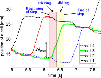
Figure 4. The sticking and sliding phases for advancing cell 3. δmax is the distance travelled by the 3rd cell from the beginning of the step until the other 3 cells stop moving backward.
Download figure:
Standard image High-resolution image3.2. Post-processing of experimental results
Before the energy expenditure of the robot can be estimated, the measured position data of the cells needs to be mined to identify the missing parameters of the system, in particular the maximum tangential deformations of the compliant contacts in forward and backward directions. For simplicity, we assume these to be equal in magnitude and denote the maximum tangential deflection in either direction by δmax. In the following, we first describe the procedure employed to identify the value of δmax of the different cells from experimental data and subsequently use this value to estimate the experimental energy expenditure of the robot.
3.2.1. Initial estimate of δmax
We begin with a visual inspection of the motion of the cells during a cycle illustrated in figure 4, in order to obtain a preliminary estimate of the maximum tangential deformation. To this end, we assume that the advancing cell begins its current step with a negative deformation of −δmax, which it has at the end of the previous step by another cell. Then, the advancing cell will stick in the initial stages of the step until reaching a deformation of δmax, at which instant it will start to slide relative to the surface. This sliding point can be identified visually, as illustrated in figure 4 for advancing cell 3, as the point at which the other three cells stop moving back. In this manner, by inspecting plots like figure 4, we identified the preliminary values of the maximum deformations for the four cells as 1.9, 1.4, 2.05 and 2.15 mm, respectively. These initial values of the maximum deformations are only approximate since they were determined from measurements of a single cycle and because the assumption that the initial deformation at the beginning of the step is −δmax may not be accurate. However, these values will serve as the starting values for the iterative procedure to compute δmax (see section 3.2.3).
3.2.2. Instantaneous cell tip deformation
As stated earlier, with the value of the maximum tangential deformation known and with the measured cell positions  one can estimate the actual deformation of the cell, i.e., the compliant leg tip, at any instant during the locomotion. First, we note that at the end of the step of the advancing cell, i.e., when it stops moving forward, the tangential deformation of that cell must be δmax (since the advancing cell slides forward). Accordingly, we can compute the location of the contact point between cell i and the surface, i.e., the location of the leg tip
  at the end of the step as:

where  denotes the position of cell i at the end of the step. Subsequently, the above contact point location will not change unless the distance between the cell and the contact point exceeds δmax, in which case sliding will occur at the cell. Thus, the criteria to identify whether a cell is sliding or sticking can be formulated as follows:

and if sliding is detected, the new position of the contact point can be estimated using δmax as:

The sign in the previous equation is chosen depending on the sliding direction of the particular cell (forward for actuated cells and backward otherwise). Based on equation (3), the contact point locations over two cycles of motion are illustrated in figure 5. Finally, the deformation associated with cell i can be estimated at any time during the locomotion according to the following:

with  measured,
  computed from (1) for the sticking phase and the value of
  identified as per sections 3.2.1 and 3.2.3. Then, the tangential contact force acting on every cell is computed by pre-multiplying the above by the tangential stiffness kt.

Figure 5. Position of contact point of each of the four cells during locomotion: a positive change means the cell slides forward and a negative change means the robot slides back. The position of the contact point is derived from the position of the cell and maximum tangential deformation.
Download figure:
Standard image High-resolution image3.2.3. Final estimate of δmax
We now refine the initial estimate of the maximum tangential deflection for our robot obtained previously in section 3.3.1. The mathematical basis for the algorithm is provided by applying the principle of linear momentum to the robot over N complete steps of motion, that is:
where P is the linear momentum, λ is the slope of the canal and Ftotal denotes the total external force applied to the device, both quantities along the direction of motion. As well, kt represents the tangential spring constant of the surface or the leg or their combination and m represents the mass of the robot. Since the robot comes to a stop at the end of each step, the above statement for the change in linear momentum can be further simplified by setting ΔP to zero. The forces acting on the robot are due to the tangential deformation of the compliant contacts between each cell and the surface and the component of robot weight along the direction of motion, i.e., mg sin(λ). With the initial estimate for δmax and the relationships established in section 3.2.2, the former can be computed explicitly at any instant during the step. Applying equation (5) to the case of horizontal crawling, thereby eliminating the weight, we obtain:

Since our experimental data is discrete, obtained at a sampling frequency fs , we employ the discretized version of the above, that is:

Using equation (7) in combination with equations (2)–(4), we search for the optimal values of  starting with the initial estimates obtained in section 3.2.1, and exhaustively searching in the interval [−0.3 mm 0.3 mm] with increments of 0.1, thus producing seven possibilities for each of the four legs. In total, 74 = 2401 possibilities were evaluated and the final solution is the one resulting in the least violation of (7), and minimum variance of Fcontact over the cycle time. The 'optimal' set of
  was found to be: 2 mm, 1.1 mm, 1.75 mm and 2.15 mm respectively for cells 1, 2, 3 and 4. To provide additional validation of these maximum deflection results, they are used to estimate the mass of the robot, again from the linear momentum principle employed for the two nonzero inclinations used in our experiments. These, together with the mean deformations are reported in table 3 demonstrating that for both slopes, the estimated weight is within 3% of the real weight of the robot. The mean deformation in table 3 is computed according to:

while the estimated mass is calculated using:

Table 3. Mean deformation and mass estimates obtained with optimal maximum deflections for different slopes and compared to actual mass of the robot (333 g).
| Slope (°) | Mean deformation | Estimated weight (g) | Error (%) |
|---|---|---|---|
| 0 | −0.008 | — | — |
| 30 | −1.71 | 342 | 2.7 |
| 45 | −2.28 | 322 | 3.3 |
3.2.4. Cell tip deformations and contact forces
Using our latest estimates of δmax and equations (1)–(4), we can now determine the tangential deformation profiles of the compliant leg tips for each cell (see figure 6). These results are presented here for the device climbing the 30° uphill. For this test case, cell 2 has the smallest δmax and the smallest deformation. From the cell tip deformations, it is possible to calculate the forces acting on the cells due to the compliance (contact forces), as well as to determine the sliding distance of the cells both forward and backward. The sliding distance allows one to calculate the energy losses, which together with the work against weight yields the total work done by the worm robot. Interestingly, the duration of sliding forward is shorter than the duration of sliding back (see figure 6, the lower nearly horizontal lines are sliding backwards whereas the higher ones are sliding forward) even though the sliding forward distance is larger (since the robot is advancing). The reason is that sliding forward of a cell occurs only when the cell is advancing; however, sliding back can occur during the whole step when the cell is not active.
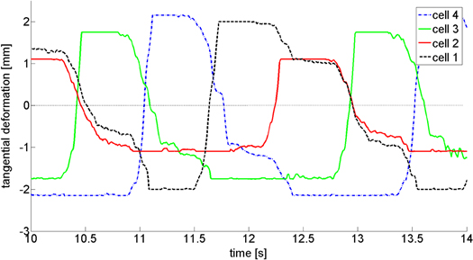
Figure 6. Estimated tangential deformation of the four cells of the worm robot climbing 30° uphill during a cycle. The tangential deformation of each cell has two intervals in which its value is nearly constant. A nearly constant positive value of the tangential deformation indicates sliding forward whereas a nearly constant negative value indicates sliding backward.
Download figure:
Standard image High-resolution image3.2.5. Actuator forces and displacements
The force acting on the actuator (or exerted by the actuator) is the sum of the elastic force acting on the cell and the component of the weight of the cell along the canal. In order to estimate the work done by the actuator, the elastic component of the actuator force must be integrated over the actuator displacement. The actuator displacement can be estimated by subtracting the motion of the actuated cell from one of the non-actuated cells. A slightly more accurate result can be obtained if we subtract the motion of the actuated cell from the average motion of the three non-actuated cells:
With all the ingredients in place, it is possible to estimate the energy consumption of the worm-robot.
3.3. Estimation of energy consumption and comparison to analysis
With the results of section 3.2, we can now employ the theoretical analysis of energy expenditure to estimate the energy expenditure of our experimental earthworm. In addition, we compare the forward and backward sliding distances per cycle, averaged over the four cells of the robot, as estimated from the experimental data (see figure 7). Two methods of computation of energy consumption are used here: one by taking the perspective of the work done against the resisting forces (energy losses), in particular, work done by sliding friction and against gravity with post-processed results as per section 3.2.4. In the second method, we directly integrate the actuator forces over the actuator displacements for each cell, which are obtained as discussed in section 3.2.5.

Figure 7. Estimated forward and backward sliding distance and comparison to theory for horizontal and 30° and 45° inclines. The bar intervals indicate the standard deviation from the average.
Download figure:
Standard image High-resolution imageConsidering the energy losses of the crawling robot, the energy consumption is comprised of the frictional losses incurred by each cell during sliding (including backward sliding) and the work done against the appropriate component of the weight over the net displacement of the robot in a cycle:

where the friction force Ff can be computed from the deformation, resulting in:

In the above, ΔX(i) denotes the amount of sliding of cell i while Lcycle represents the measured net displacement of the robot. On the other hand, the work input computed by integrating the actuator force over its extension, for all cells becomes:
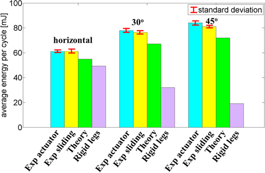
For a particular experiment (horizontal canal or sloped canal), equations (11) and (13) were employed to determine the energy consumption for every cycle (approximately ten cycles for each experiment) and the corresponding averages and standard deviations were computed. Figure 7 presents the sliding distances in the forward and backward directions as expected from the theory and compared to the experimental estimates. The robot is sliding both forward and back by more than predicted by the theory. For example, the backward sliding on the horizontal surface is more than 1 mm/cycle whereas no sliding is predicted. The reason behind this is that since some of the clamps are exerting less normal force, they are more likely to slide (both forward and back) resulting in a larger sliding distance. Note that the energy dissipated by sliding is the product of the normal force times COF times the distance. Therefore the clamps that exert less normal force will dissipate less energy when sliding. Figure 8 presents the results for the experimental energy consumption estimates computed with equation (11) (Exp. sliding) and (13) (Exp. actuator). Also included is the theoretical value of energy consumption which differs from the computation of the experimental values in two respects. First, the value of δmax employed to obtain the theoretical values was taken as the average of δmax identified for each leg in the experiments. Second, the value of the net displacement of the robot, Lcycle, is evaluated using the analytical predictions (Zarrouk et al 2012a). The net displacement values are summarized in table 4 for the horizontal and two sloped canals.
Figure 8. Estimated energy requirement, including sliding losses and potential energy, per cycle for horizontal and 30° and 45° inclines based on equation (11) and (13). The bar intervals indicate the standard deviation of the results.
Download figure:
Standard image High-resolution image
Table 4. Net robot displacement in one cycle.
| Slope (°) | Lcycle theoretical (mm) | Lcycle measured (mm) |
|---|---|---|
| 0 | 6.83 | 7.18 |
| 30 | 4.61 | 3.76 |
| 45 | 2.08 | 2.08 |
Several observations can be made based on figure 8: (i) the two methods of computing the experimental energy consumption are in excellent agreement with each other and exhibit low standard deviations, pointing to good repeatability of the results; (ii) the energy consumption observed in the experiments is in very good agreement with the theoretical predictions, as expected, with discrepancies between the two of approximately 15%; (iii) the energy consumption computed by neglecting the compliance at the contact between the robot and environment progressively underestimates the real consumption as the slope increases. Note that since the total energy consumed is the combination of the energy dissipated in sliding (sliding distance times normal force times COF) together with work against gravity, the energy errors observed in figure 8 are relatively smaller than the errors observed in the estimated sliding distance in figure 7.
4. Conclusions
Worm robots are being proposed for a range of applications, some of which involve compliant contact conditions. The contact compliance can be due to the properties of the canal (e.g., compliant tube) or as part of the device clamping mechanism which may be equipped with compliant tips to increase friction and reduce collisions. In our previous work (Zarrouk et al 2012a), it was demonstrated that this compliance reduces the distance travelled per cycle. An extreme example of this is a worm-robot which can climb vertically when the contact conditions are rigid, but cannot climb beyond 45° slope when there is compliance at the interface between the robot and the environment. In the present paper, the compliance was introduced at the leg tips, which may be necessary for safety reasons or to represent the flexibility of the robot legs themselves; the leg tip compliance can also approximate the local compliance of the environment. The locomotion energy requirements were derived analytically in (Zarrouk et al 2012c). The latter were used to predict the amount of energy required to travel a given distance. For the minimum work requirements, the expressions were formulated by summing the net work done by the worm robot and the energy losses due to friction at the contact points. In this manuscript, we reported on the results of experiments conducted with a four-cell earthworm robot with compliant tips. Using the compliance values of the contact between the leg tips and environment, together with the position of the cells measured during locomotion, we were able to estimate the sliding distance of the cells and the sliding friction forces. These in turn were used to calculate the experimental energy losses during locomotion and the total energy requirements. The experimental results were within 15% of the theoretical predictions of the energy per cycle. Comparison to the theoretical energy consumption results for a robot with rigid contacts showed a substantial effect of contact compliance on the energetics of locomotion, with the energy requirements nearly a factor of four higher for climbing on a 45° slope.