
Abstract
Objective. The use of an electroencephalogram (EEG) anticipation-related component, the expectancy wave (E-wave), in brain–machine interaction was proposed more than 50 years ago. This possibility was not explored for decades, but recently it was shown that voluntary attempts to select items using eye fixations, but not spontaneous eye fixations, are accompanied by the E-wave. Thus, the use of the E-wave detection was proposed for the enhancement of gaze interaction technology, which has a strong need for a mean to decide if a gaze behavior is voluntary or not. Here, we attempted at estimating whether this approach can be used in the context of moving object selection through smooth pursuit eye movements. Approach. Eighteen participants selected, one by one, items which moved on a computer screen, by gazing at them. In separate runs, the participants performed tasks not related to voluntary selection but also provoking smooth pursuit. A low-cost consumer-grade eye tracker was used for item selection. Main results. A component resembling the E-wave was found in the averaged EEG segments time-locked to voluntary selection events of every participant. Linear discriminant analysis with shrinkage regularization classified the intentional and spontaneous smooth pursuit eye movements, using single-trial 300 ms long EEG segments, significantly above chance in eight participants. When the classifier output was averaged over ten subsequent data segments, median group ROC AUC of 0.75 was achieved. Significance. The results suggest the possible usefulness of the E-wave detection in the gaze-based selection of moving items, e.g. in video games. This technique might be more effective when trial data can be averaged, thus it could be considered for use in passive interfaces, for example, in estimating the degree of the user's involvement during gaze-based interaction.
Export citation and abstract BibTeX RIS

Original content from this work may be used under the terms of the Creative Commons Attribution 4.0 license. Any further distribution of this work must maintain attribution to the author(s) and the title of the work, journal citation and DOI.
1. Introduction
As early as in 1966, Grey Walter, most known for his discovery of the E-wave (expectancy wave) in the human electroencephalogram (EEG), proposed to use this EEG component for 'the direct cerebral control of machines' (Walter 1966). Notably, the proposed system included not only an E-wave detector but also a separate detector of the motor-related readiness potential. This early sketch of a brain–computer interface (BCI) was unfortunately forgotten. However, the E-wave itself became one of the most popular phenomena studied by psychophysiologists, typically as a part of the contingent negative variation (CNV; this term was also proposed by Grey Walter), which is a more complex EEG phenomenon that also includes motor components. (Instead of the term 'E-wave', another term, 'stimulus preceding negativity', SPN, is sometimes used, e.g. Boxtel and Brunia 1994, Brunia and Van Boxtel 2001, Pornpattananangkul et al 2017. Quite often, only the term CNV is used, without differentiation of the subcomponents. Here, we use the original term 'E-wave' for the EEG component related not to motor preparation but only to expectation/anticipation of a forthcoming stimulus, as a tribute to Grey Walter's early studies and insights.) Only recently, the CNV was employed in a few neuroengineering studies not directly related to intentional control, namely as a mean to detect the cognitive state of anticipation and to predict actions in simulated driving scenarios (Khaliliardali et al 2012, 2015, Guo et al 2019).
The approach to use the E-way for the control of machines in its original form (Walter 1966) implied a paradoxical way of acting by expecting the effect of action ('thus by-passing the operant effector system'). It was reinvented by Thorsten Zander's group, who aimed on solving the critical problem of another human-machine interaction technology, the gaze-based control. This problem, called the Midas touch problem, is the inability of eye tracker-based human-machine interfaces to differentiate, in many cases, voluntary eye behaviors used for input from spontaneous ones, e.g. those used for visual scene exploration (Jacob 1991). One of the most usual ways to communicate or control computers with such interfaces is to use relatively long eye fixations, or, more exactly, gaze dwells on certain 'sensitive' screen objects, e.g. keys of a screen keyboard, on-screen buttons, internet links, etc (Majaranta and Bulling 2014). (In the gaze interaction literature, the term 'fixation' is often used. In the eye movement literature, however, this term is related to a time interval when an eye is still, i.e. eye movement velocity is near zero, while algorithms used in gaze-sensitive interfaces usually rely not on eye velocity but on spatial criteria, such as the presence of the gaze in a certain area for a certain time. The dwell is exactly the term for the eye-gaze behavior that corresponds to such spatial criteria, see Holmqvist et al 2011, section 6.3.2.) Numerous solutions proposed for the Midas touch problem all suffered from imposing significant demands on the user (e.g. use of too long dwell time, or additional actions to confirm a selection; see Velichkovsky et al 1997, Majaranta and Bulling 2014, for reviews). Ihme and Zander (2011) and Protzak et al (2013) noticed that during the intentional gaze dwells the user of such interfaces anticipates a feedback from the interface, an indication that the command was executed, and proposed to enable triggering only when triggering is anticipated. Unlike in other hybrid interfaces where the gaze is used together with a BCI (Zander et al 2010, Kim et al 2015), the BCI here makes use of brain activity anyway produced during gaze-based interaction, so it does not require any additional action from the user. In the terms of the dichotomy of explicit interaction/active interfaces vs. implicit interaction/ passive interfaces (Zander and Kothe 2011, Krol et al 2020), human–machine interaction enabled by such an interface is explicit to the user, while its BCI component supports gaze-based control implicitly to the user, without their awareness—therefore, not claiming additional cognitive resources. We call this interface the eye–brain–computer interface (EBCI), as it is based on a high integration of its eye and brain components' function.
In their experimental studies simulating such EBCI, Ihme and Zander (2011) and Protzak et al (2013) demonstrated that the EEG collected during gaze dwells under the anticipation of the feedback and without such anticipation indeed can be successfully classified. However, their experiment tasks required that the participants had to find a target among non-targets. It was shown that the EEG recorded in visual search tasks and in tasks where participants look at items of different relevance to them, can help to identify the target or to measure relevance, especially due to the P300 wave, which leads to the development of a specific type of passive hybrid BCIs (Kamienkowski et al 2012, Brouwer et al 2013, Putze et al 2013, Jangraw et al 2014, Ušćumlić and Blankertz 2016, Putze et al 2016, Wenzel et al 2017, Golenia et al 2018, Salous et al 2018, Jacucci et al 2019). The P300 wave is associated with the relevance of the stimulus and the uncertainty about it. In these studies, participants did not know the location of the relevant items in advance, which apparently made possible the development of the P300 when they found the items. While these systems may have important applications, they are a different technology. Note that while the EBCI by Zander's group included a passive BCI component, the whole system was designed for the purpose to actively communicate the user's intention rather than automatically inform about what is relevant to them.
In many scenarios of typical graphical user interface use, the user has prior knowledge of the locations of the items used for control (e.g. screen buttons). It is unlikely that an EEG classifier trained to use the P300 features will be helpful in such scenarios, due to lack of prior uncertainty and, therefore, lack of the P300. In addition, voluntary selection with gaze can be needed when the item to be selected is not much more relevant (if any) than other items. Thus, for supporting voluntary interaction it is important to ensure that a BCI can discriminate voluntary and spontaneous gaze dwells without using the P300 wave.
Thus, it was important to demonstrate that an E-wave based EBCI can differentiate eye dwells voluntary used for control from spontaneous ones even if the targets are chosen freely by a user. For this purpose, Shishkin et al (2016) recorded EEG in participants who were asked to play a gaze-controlled computer game. When choosing the game and creating instructions for this study, the authors ensured that the participants typically knew an object's position prior to starting gazing at it for selection, so the appearance of the P300 wave was unlikely. The dwell time threshold was set to 500 ms (significantly shorter than in Ihme and Zander 2011, Protzak et al 2013), which made interaction comfortable enough and did not prevent immersion in the game playing. To make a move, the participant had to switch on the gaze-based control by an eye dwell on a special remote object. Dwells that followed this action were considered voluntary (intentional), while dwells not preceded by it were deemed spontaneous. As expected, voluntary, but not spontaneous, dwells were accompanied by a typical E-wave (in the paper, the term 'stimulus-preceding negativity', was used). While components typical to target-related EEG in visual search and relevance studies (such as P300) did not appear during voluntary dwells, it was successfully classified against the EEG accompanying spontaneous dwells (Shishkin et al 2016). This EBCI design was further tested in an online study (Nuzhdin et al 2017).
In the above-cited studies, the visual displays of the gaze-sensitive user interfaces were stable, without moving objects, as in the vast majority of such interfaces used in studies and in commercial systems. Relatively recently, the selection of moving objects with smooth pursuit eye movement was found to be highly effective, in addition to the long-used gaze fixations (dwells) and saccades (Vidal et al 2013, 2015). Smooth pursuit eye movement can be viewed as 'dynamical' fixations on moving objects. It is initiated and maintained in response to a smoothly moving target easily and mostly automatically, without subjective effort (Lisberger et al 1987, Brielmann and Spering 2015). Smooth pursuit eye movement can therefore enable interaction without the need for calibration (Pfeuffer et al 2013). Basically, the correlations of eye movements with the trajectories of moving objects are computed and the object with the highest correlation is assumed to be the one the user is looking at. Because smooth pursuit is quite precise, this technique is especially appealing as a solution for small displays, such as smart watches, where gaze-sensitive objects cannot be separated at distances large enough to make it possible to reliably differentiate dwells on them (Esteves et al 2015). Also, the application of the smooth pursuit eye movement has been found in text entry (Hans-Martin Lutz et al 2015), PIN code entry (Cymek et al 2014, Liu et al 2015), and even in virtual reality (Khamis et al 2018).
In the presence of multiple moving objects, any of such objects can easily attract attention and become pursued with gaze automatically, and the Midas touch problem may become aggravated. Again, it seems reasonable to overcome it by adding expectation detection to the interface for moving object selection. However, only experimental studies can show if this is feasible, as multiple factors may change EEG components in such dynamical settings (see discussion on such factors in Ganin et al 2013, Shishkin et al 2011). Smooth pursuit eye movement was investigated in the basic studies of vision and attention (e.g. Schütz et al 2011). The EEG accompanying smooth pursuit eye movements was studied far less, and typically using stimuli presented on moving objects, again with the purpose of studying specific fundamental questions, such as attention allocation (e.g. Chen et al 2017), or with the focus on the P300 BCI development (Shishkin et al 2011, Ganin et al 2013). Moving object tracking did not influence EEG classification both in the stimulus-based P300 BCI paradigm (Shishkin et al 2011, Ganin et al 2013) and in the stimulus-free EEG-based target decoding (Ušćumlić et al 2015), but cognitive processes in these cases and in intentional selection using gaze are quite different. We found no prior studies of EEG accompanying intentional object selection with smooth pursuit eye movement.
In our preliminary studies (Zhao et al 2018a, 2018b) we observed an E-wave-like EEG component prior to moving object selection with gaze, but a similar wave also accompanied smooth pursuit eye movement in control conditions, where the intention to select an object could not appear. We concluded that a certain form of expectation or at least estimation of time to execute certain operations (a related cognitive activity) easily appears under various conditions when the pursuit is intentionally used to follow an instruction. In the current study, we designed a control condition that was free from this shortcoming and corrected some other details of the study design. With the new design, we collected data from a larger group of participants, which allowed us to analyze the difference between the EEG accompanying spontaneous smooth pursuit and intentional selection of moving objects with gaze, and also to model their classification in the framework of an EBCI using a convolutional neural network.
Earlier versions of this study were reported at a few conferences (Zhao et al 2019a, 2019b, 2019c). We also enhanced EEG preprocessing with the independent component analysis (ICA); replaced the neural network classifier used in these earlier versions by the linear discriminant analysis with shrinkage regularization (sLDA), which produced more stable results when trained on small samples and allowed for easier interpretation of feature involvement into classification; and conducted a number of additional analyses, such as evaluating the effect of averaging data from sequential trials and estimating the possible contribution of oculographic artifacts.
2. Methods
2.1. Participants
Twenty healthy volunteers (11 male, 9 female), aged 20–52 (M ± SD 27 ± 7) years participated in the study after being introduced to the procedure and signing an informed consent. The experiment was performed according to the Helsinki Declaration and with the approval of the local ethical committee. Four of the participants (#1, #2, #3, #15) participated in two sessions on different days, while others participated each in a single session. Thirteen participants had prior experience with gaze-based control of a computer. Fourteen participants had normal vision and the others had corrected to normal vision.
2.2. Data acquisition
A consumer-grade eye tracker Tobii 4 C (Tobii, Sweden) with a 90 Hz frame rate was attached to the lower edge of the 18.5'' LCD monitor with a screen resolution of 1440 × 900 and 75 Hz refresh rate. EEG was recorded from 19 locations (F3, Fz, F4, C3, Cz, C4, P1, P3, Pz, P2, P4, PO7, PO3, POz, PO4, PO8, O1, Oz, O2) with 0–200 Hz bandpass at 500 Hz sampling rate and 24-bit voltage resolution with NVX52 DC system (MCS, Russia). In the studies of the gaze-based selection of static objects the EEG marker of voluntary (intentional) selection (the E-wave) was typically found in the occipitoparietal region (Shishkin et al 2016, Nuzhdin et al 2017), thus more electrodes were placed in the posterior area than in the anterior one. Reference EEG electrodes were digitally connected earlobes. The electrooculogram (EOG) was recorded with the same amplifier using electrodes placed near the outer canthi for recording the horizontal component of eye movement, and above and below the right eye for recording the vertical component. The ground electrode was placed at the Fpz position. Impedance was kept below 20 KOhm. In nine participants (##11–20) a sound signal from a microphone was recorded with the same amplifier to enable detection of time periods when the participants reported their answers (in task CT, see below). The microphone was placed about 10 cm below the mouth to avoid artifacts from breathing.
2.3. Task
The participants were presented with 15 'balls' (circles) displayed on a monitor screen (figure 1). The ball diameter was 80 px, subtending 2.1° at screen distance, which was about 64 cm from the participants' eyes. The balls were numbered from 1 to 15 and contained 5–8 dots around the number (figure 1). In the 'dynamic' conditions (select moving balls (SMB), find accelerated (FA), counting task (CT), see below), balls moved linearly on the screen at a speed ∼230 px s−1 (6° s−1), changing their movement direction in a natural way when hitting each other or the screen edges. In the 'static' condition (select static balls (SSB)), they did not move.
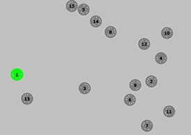
Figure 1. A screenshot of a typical experimental layout. Note that all the 'balls' were static in one experimental condition (SSB) and all moved in other conditions (SMB, FA, CT). The screenshot was made when ball #1 was selected by gaze and therefore highlighted with green color, to provide a visual feedback for the selection. Highlighting was used in the SMB and SSB conditions, while in the FA and CT conditions all balls stayed gray all time.
Download figure:
Standard image High-resolution imageBefore an experiment, 10 sets of 15 ball images were generated. Each set consisted of 15 images. On 3 of them, there were 5 dots, and on 4 images each were 6, 7 and 8 points. Images with the same number of dots differed in their positions, which were set randomly. At the start of an experimental block (corresponding to one of four experimental conditions, see the description of the procedure below), one set of images was randomly chosen and numbers from 1 to 15 were randomly assigned to each ball (see an example in figure 1). For the next block, the image set was changed into another random one.
After completing a block, the set of images with dots was changed into another random one. Ball positions in the SSB (static balls) condition and their initial positions in other (moving balls) conditions were tied to invisible grid cells (the number of cells matched the number of balls), with random horizontal and vertical shifts relative to the cell centers.
In a run, the participants were asked to complete one of the following tasks (corresponding to four conditions):
Select moving balls (SMB)—select the 15 moving balls one by one according to their numbers in ascending order and then (only for the participants ##7–14) in descending order (see details about the selection below).
Select static balls (SSB)—select 15 balls one by one as in the SMB condition, but in this case, the balls were fixed at their initial positions.
Find accelerated (FA)—find the ball that was moving faster than the other balls. This target ball, randomly chosen, accelerated once after 15–20 s from the block start by 1.3° s−1 (19% of the basic speed), while the rest of the balls continued to move without changing their speeds (6° s−1). Participants were advised to announce the number of the ball that appeared to be the accelerated one only when they made sure that it was indeed faster than the others.
Counting task (CT)—find moving balls with a specified number of dots and summate the balls' numbers. In this condition, participants were asked, five times in a row, to find a ball with the number of dots specified by the experimenter (this number could be from 5 to 8, chosen randomly each time). After finding an appropriate ball they had to summate its labeling number with the number(s) of the previous ball(s). Dots were not used in other conditions, but they were presented in all conditions to ensure visual equality of the displays across conditions.
The SMB and SSB tasks modeled voluntary (intentional) gaze selection. In contrast, FA and CT tasks modeled a situation where smooth pursuit eye movement can appear without intention to select, while the visual display was exactly the same as in the SMB task. The SMB task was similar to the task used in (Isachenko et al 2018) where the gaze-based selection was compared to mouse-based one. However, in the current study, the number of balls and their speed were set at a lower level, otherwise, FA and CT tasks appeared to be too difficult.
2.4. Online gaze-based selection
At the beginning of a run, all the balls were dark gray (see figure 1). In the SMB and SSB conditions, gazing at a ball for a certain time leads to its 'selection': the selected ball was highlighted with green color. Ball color returned to dark gray when another ball was selected. In the FA and CT conditions, the balls never changed their color. However, the online algorithm underlying the selection operated in the FA and CT conditions exactly as in the SMB and SSB conditions with the only difference that its triggering did not lead to ball color change.
In all conditions, the median distance from the gaze position to each ball's center was calculated in a moving window of ∼867 ms length. If this measure computed for a ball did not exceed 55 px (in other words, the distance did not exceed 55 px longer than half of this length) and was the smallest among all balls, this ball was selected. Some samples from the eye tracker (sampling rate 90 Hz) were discarded from time to time to maintain synchrony with the monitor (its refresh rate was 75 Hz). Using a high-speed (240 fps) video camera and a mirror we found out that a delay between a saccade onset and display response in our settings was approximately 140 ms. (In this test, the display response was observed in a form of the movement of a cursor controlled by the gaze coordinates. The cursor was used only for tuning the system and it was not presented in the experiments). To improve synchronization between the gaze and balls coordinate streams (which was important for correct selection), the latter streams were intentionally delayed by 140 ms. The eye trackers' built-in alignment filter was not applied. With a few exceptions, the selection algorithm followed one described in Isachenko et al (2018).
Selection triggering time was recorded along with the EEG using a photosensor attached to the lower-left edge of the screen, where a circle not visible to a participant changed its brightness as the algorithm triggered. In the SMB and SSB conditions, this change happened in the same video frame when the visual feedback started (a selected ball changed its color). The number of the ball selected by the algorithm was recorded, regardless of whether or not it was visually highlighted.
The visual task and selection algorithm were implemented in C++ and QML with the use of the Qt framework.
2.5. Procedure
Participants were seated in an adjustable chair in front of an office table with the monitor. To ensure head position stabilization a chin rest and a forehead rest were used.
The experiment consisted of six blocks. Each block contained all four conditions (figure 2). The order of conditions was the same over blocks for a single participant but counterbalanced in the group of participants. Conditions, where balls were intentionally selected with gaze (SMB, SSB), were not allowed to immediately follow each other. Each condition in a block included one run of ∼2 min duration.
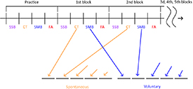
Figure 2. Experiment timeline. The order of conditions (SSB, CT, SMB, and FA) was fixed across blocks and randomized across participants. In the bottom, the formation of the dataset for classification is shown for the case of using the SMB as the voluntary class (for the SSB, the approach is the same).
Download figure:
Standard image High-resolution imageBefore the start of the first block, the experimenter showed the moving balls and in detail explained the tasks. The first block was considered as practice, and the participants were allowed to ask any questions during the runs. The data from the subsequent five blocks were used for analysis.
Before each block, native seven-points calibration of the eye tracker was used. In the SMB and SSB conditions, if the experimenter noticed that the participant experienced problems with selection or the participant themselves reported such problems, the eye tracker was recalibrated and the run was overwritten. Within a single block, participants were asked to avoid movements to prevent calibration distortion. After completing one block, the participants were allowed to rest for a few minutes. Ten minutes break came after the third block.
Participants were instructed that they should try to avoid the selection of the wrong balls (with a number different from what was the current target), but if such selection happened, they should continue an attempt to select the ball with the number next to the previous correct selection. They were also told not to hurry with selection and be focused on the task.
In FA and CT conditions, participants were not aware of the online detection of their smooth pursuit eye movement. Thus, these conditions represented the case when the user triggers a gaze-sensitive system unintentionally. FA task was already employed in our preliminary studies (Zhao et al 2018a, 2018b), where some negative deflection resembling the E-wave was observed in the averaged trigger-related EEG time courses for this task. It was proposed that this negative deflection could be related to the expectation of the moment where a ball that a participant watched as a candidate for the target came close to another ball, which was helpful for comparing their speeds (remember that FA task was to find the ball which moved slightly faster than all the others). Thus, the 'counting' task, CT, was designed, in such a way that anticipation was excluded. In the current study, the CT task was added to the study design as the main condition for provoking spontaneous smooth pursuit. The FA condition was still kept in the design, to represent a significantly different case of the involuntary triggering of a gaze-sensitive system.
At the end of an experiment, participants were asked to rate how difficult it was performing a task by putting a mark on four visual analog scales, one per condition, placed on a single sheet of paper (so that the previous mark(s) could be used as a reference for the new one(s)). The left end of the scale was labeled 'very easy' and the right end was labeled 'very difficult'.
2.6. EEG preprocessing
All EEG analysis was made offline using the data collected during the experiments. EEG data were filtered with zero-phase lowpass 4th order Butterworth filter with a cutoff frequency of 30 Hz. EEG segmentation was based on triggers in the photodiode channel, which corresponded to algorithm triggering (see above the description of online gaze-based selection). One triggering was considered as constituting one trial, irrespective of the nature of smooth pursuit or gaze dwell that could cause it (voluntary attempt to select, as in SMB and SSB conditions, an attempt to estimate a ball's speed, or pursuing a ball while counting dots on it). EEG/EOG epochs −1200 ... +1200 ms relative to the trigger were extracted.
In addition to direct use of the time of online gaze-based selection algorithm triggering as reference (zero) time, we also made an alternative set of segments from the same raw EEG related to pursuit onset. As its direct estimation is a complicated task, we used as the reference time the time of gaze landing prior to the pursuit (or the static dwell, in the SSB condition). Since our Tobii eye tracker license did not allow for gaze coordinate collection and offline analysis, this time was found using gaze velocity extrapolated from the EOG prior to the online triggering. The following heuristic procedure was used:
- (a)Compute vertical and horizontal components of eye velocity as the first derivative of the vertical/horizontal EOG (VEOG/HEOG) signals (i.e. vertical/horizontal eye velocities).
- (b)Find the saccade with peak velocity above 5 × average velocity ('large saccade') closest to −450 ms before online triggering.
- (c)If a saccade corresponding to (2) not found, find the saccade with peak velocity above 2 × median velocity ('small saccade') preceding the online triggering and closest to it.
- (d)Estimate saccade end time as the time where the eye velocity falls to 1.5 × average velocity.
Most commonly HEOG and VEOG were used concurrently. If VEOG was noisy and its derivative did not contain peaks, only HEOG was used. If no peaks in EOG derivatives were detected near dwell onset, the trial was rejected from the subsequent analysis.
2.7. Artifact removal and rejection
Components associated with eye movements were removed from the EEG signal through the ICA using runica algorithm (based on Infomax ICA) with the default settings in the EEGLAB package (Delorme and Makeig 2004). ICA was applied to concatenated segments of the EEG and EOG signals from all conditions, for each participant separately, and produced 21 independent components. To determine which of them had the oculomotor origin, we separately calculated the Pearson correlation coefficient between the component activations and the vertical and horizontal EOG. Visual inspection of component projection topographic maps and activation time courses using the EEGLAB functions showed that components with a correlation coefficient larger than 0.3 with either HEOG or VEOG were indeed related to the oculomotor activity. Two to three components per participant met this criterion and were rejected.
Finally, trials were discarded from analysis if any of the following criteria were met:
- (a)Error in selection order (from 1 to 15 forward and backward) (SMB and SSB only).
- (b)The pursued ball was the accelerated ball (FA only).
- (c)Pursuit/dwell duration was shorter than 450 ms or longer than 1200 ms.
- (d)Absolute amplitude higher than 150 µV in any EEG or EOG channel in −300 to 0 ms interval relative to selection triggering (for the event-related potential (ERP) analysis and classification) or 150 to 450 ms interval relative to pre-pursuit saccade end (for the ERP analysis only), depending on which of these events were used as zero time for ERP analysis and for feature extraction.
- (e)Absolute amplitude of sound signal exceeded an empirically tuned threshold (participants ##11–20 only) in −500 to 0 ms interval relative to selection triggering
Criterion (a) enabled removing selections that occurred due to a participant's mistake or false algorithm triggering, which could not be considered as voluntary selections.
Criterion (b) was designed to reduce the number of trials in which participants compared the speed of the accelerated ball and the nearest balls, when an E-wave could arise due to anticipation of the moment where such comparison could be made (such attempts seemed to be especially frequent in the case of pursuing the accelerated ball).
Criterion (c) served to remove false positive selections that could happen due to accidental closeness of a ball to gaze position before the pursuit and trials with too late selection algorithm triggering due to calibration issues or loss of eye focus.
Criterion (d) served to reject trials with artifacts, such as related to remaining EOG or muscle activity.
Criterion (e) enabled rejection of trials where the participant gave spoken response (in FA and CT) already within the trial, which could significantly change the EEG signal. (Microphone recording was absent in the first half of the participant group, so this criterion could not be applied to their recordings. However, comparison of the averaged ERPs obtained with and without application of this criterion showed little difference, so we decided to use together with the recordings from the first half of the group preprocessed without this criterion and the recordings from the second half of the group to which the criterion was applied.)
The criteria were applied, in the order specified above, separately to the recordings preprocessed and not preprocessed by ICA, and separately for using selection triggering and pre-pursuit saccade end as zero time. In case of using selection triggering as zero time rejection rate over the group was, per condition: for the signals not preprocessed with ICA, 24.6% (SMB), 14.5% (SSB), 32.5% (FA), 37.8% (CT); for the ICA-preprocessed signals, 23.3% (SMB), 12.9% (SSB), 26.7% (FA), 31.3% (CT), leaving the following final number of epochs per participant (min-max) and condition: 48–181 (SMB), 50–174 (SSB), 26–117 (FA), 32–169 (CT). (In case of using pre-pursuit saccade end as zero time, the number of epochs was only slightly different from the above figures.) The individual number of epochs per participant for SMB, SSB, and CT conditions (used for the analysis of classification performance) are presented in the Results section (table 1).
Table 1. The number of epochs per condition used for EEG analysis and the classification results for sLDA applied to the ICA-cleaned EEGs. SMB and SSB are voluntary selection experiment conditions, CT is a control condition where the smooth pursuit was not related to the intention to select. P-values (uncorrected) were computed for the ROC AUC values using a permutation test (p < 0.05 are shown in bold). Med.—median, MAD—median absolute deviation.
| ID | N of epochs | ROC AUC | |||||
|---|---|---|---|---|---|---|---|
| SMB | SSB | CT | SMB vs. CT | p-value | SSB vs. CT | p-value | |
| 1 | 60 | 72 | 73 | 0.50 | 0.516 | 0.66 | <0.001 |
| 2 | 100 | 131 | 98 | 0.50 | 0.494 | 0.57 | 0.040 |
| 3 | 129 | 128 | 96 | 0.58 | 0.036 | 0.62 | 0.001 |
| 4 | 48 | 50 | 46 | 0.59 | 0.067 | 0.49 | 0.538 |
| 5 | 55 | 65 | 96 | 0.64 | 0.005 | 0.52 | 0.300 |
| 6 | 70 | 73 | 151 | 0.51 | 0.397 | 0.71 | <0.001 |
| 7 | 181 | 174 | 163 | 0.59 | 0.003 | 0.58 | 0.007 |
| 8 | 156 | 171 | 169 | 0.53 | 0.173 | 0.59 | 0.002 |
| 9 | 137 | 138 | 155 | 0.54 | 0.136 | 0.54 | 0.141 |
| 10 | 124 | 139 | 90 | 0.57 | 0.041 | 0.68 | <0.001 |
| 11 | 141 | 140 | 74 | 0.52 | 0.375 | 0.66 | <0.001 |
| 14 | 133 | 137 | 92 | 0.63 | <0.001 | 0.62 | 0.003 |
| 15 | 125 | 136 | 47 | 0.45 | 0.775 | 0.50 | 0.487 |
| 16 | 127 | 134 | 43 | 0.75 | <0.001 | 0.66 | 0.004 |
| 17 | 123 | 127 | 69 | 0.61 | 0.017 | 0.58 | 0.040 |
| 18 | 101 | 100 | 32 | 0.61 | 0.054 | 0.43 | 0.836 |
| 19 | 117 | 138 | 43 | 0.66 | 0.006 | 0.56 | 0.183 |
| 20 | 109 | 135 | 52 | 0.41 | 0.934 | 0.46 | 0.778 |
| M | 113.1 | 121.5 | 88.3 | 0.57 | 0.58 | ||
| SD | 35.7 | 35.1 | 44.5 | 0.08 | 0.06 | ||
| Med. | 123.5 | 134.5 | 82 | 0.58 | 0.58 | ||
| MAD | 16 | 6 | 32.5 | 0.06 | 0.06 | ||
The resulting dataset was used for the EEG analysis and classification.
Signal preprocessing, statistical analysis, and visualization were performed using MATLAB (MathWorks, USA). Function topoplot from the EEGLAB package (Delorme and Makeig 2004) was used to create topographical amplitude maps.
2.8. Feature extraction
For the classification, data from the SMB (voluntary pursuits), SSB (voluntary dwells), and CT (spontaneous pursuits) conditions were used. In one analysis, we classified SMB vs. CT, and in another one, SSB vs. CT. The FA condition could not be considered as typically unintentional behavior of the participants due to pronounced similarity to the SMB condition (figure 3), so the classifier was trained and tested on both intentional conditions only against the CT condition.
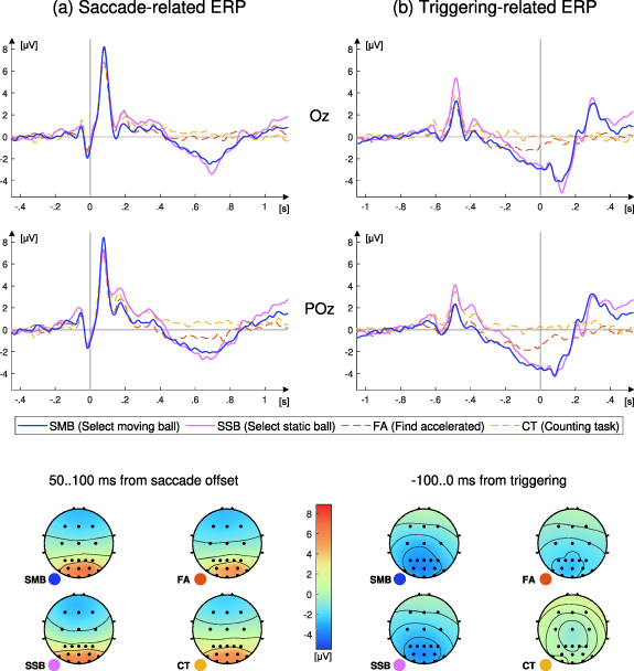
Figure 3. Time courses at POz and Oz electrodes (upper and middle rows) and topographical maps (bottom row) of the grand average event-related potentials (N = 18) time-locked to the end of the last saccade (or microsaccade) before the pursuit or (in SSB condition) dwell (a), and to gaze-based selection algorithm triggering (b). Four colors of the lines correspond to four experiment conditions (SMB, SSB, FA, CT). The baseline was −500 to −200 ms relative to the saccade end (a) and −1000 to −700 ms relative to the triggering (b). Visual feedback was provided to the participants at triggering in SMB and SSB but not in CT and FA conditions. Time scale in (b) was corrected for the delay between actual triggering and the feedback, so that zero time in (b) corresponds to feedback onset. The EEG was cleaned from the EOG potentials using ICA.
Download figure:
Standard image High-resolution imageFigure 2 shows how the voluntary and spontaneous classes were formed from the data recorded in different blocks.
Number of epochs per class was balanced for each participant separately in pairs of classes, SMB vs. CT and SSB vs. CT, towards a class with less number of epochs. To do this, before classification, some epochs were randomly removed from a class with a larger number of epochs so that the number of epochs in both classes got matched.
Mean amplitudes of 20 ms length adjacent time windows in the −300 to 0 ms interval relative to selection triggering were used as features (15 windows per channel). This time interval was chosen for the following reasons. We expected, based on the averaged fixation-related potentials in the case of static object selection (Shishkin et al 2016), that the expectation-related brain activity will manifest itself as a slow negative-going deflection, most pronounced close to the time of selection triggering. However, earlier in the pre-triggering interval other EEG phase-locked components could be observed. One of them should be the lambda wave, a post-saccade positive peak (Thickbroom et al 1991, Kazai and Yagi 2003). It is well-developed after saccades in free-viewing conditions (Kamienkowski et al 2012, Nikolaev et al 2016, Ries et al 2018) and even after microsaccades (Dimigen et al 2009). This component is highly sensitive to factors irrelevant to intention (Nikolaev et al 2016). Inspection of the triggering-related ERP (figure 3(b)) showed that in our data the lambda-wave latency was about −500 ms. Due to its jitter relative to the triggering time, it could likely affect intervals closer to the triggering. Hence, we decided to extract features not earlier than −300 ms, to avoid contamination from the lambda wave. The right border of the interval for feature extraction was set at 0 ms, due to the need to simulate online application of the BCI, which prevented the use of features taken later than triggering of the interface. In addition, possibly remaining ocular artifacts should be not pronounced between −300 ms and 0 ms.
Mean amplitude of the −100.0 ms (relative to online gaze-based selection triggering) baseline interval was subtracted from the EEG amplitudes channelwise to remove drifts in the data (note that we did not use a high pass filter, to prevent the distortion of the relatively slow E-wave). We expected that subtracting the baseline mean should make the amplitude features sensitive to the slope of the E-wave. In our earlier work with the selection of static objects (Shishkin et al 2016), we found that the traditional placement of the baseline interval outside the interval of interest is questionable in the case of gaze-based selection, because the EEG in most of the neighboring time is strongly affected by oculographic artifacts. Placing the baseline at the interval where the highest amplitude of the E-wave was expected made the neurophysiological interpretation of the results even more counterintuitive, but it was necessary because earlier pre-feedback intervals could be more affected by coulomotor artifacts or include irrelevant fixation-related EEG components (e.g. the P300 wave and even the lambda wave; note that the jitter in their latencies relative to the selection triggering could lead to their moving into the interval, from which the features were extracted, in some trials).
Features from all EEG channels were concatenated, forming a vector of 19 × 15 = 135 features for a single epoch.
2.9. Classification
We used linear discriminant analysis with shrinkage regularization implemented in Fieldtrip toolbox for EEG/MEG-analysis (Oostenveld et al 2011, www.ru.nl/neuroimaging/fieldtrip), further referred to as sLDA (shrinkage LDA). The sLDA was trained and tested on SMB vs. CT trials, representing voluntary and spontaneous smooth pursuit data, respectively. Additionally, a more distinct data, SSB trials (voluntary dwells) were classified also against CT, as a complementary indirect control of the contribution of eye movement to classification. Five-fold cross-validation was used for the estimation of the classifier performance. Folds were formed blockwise (without overlap in time). Specifically, the dataset, separately for voluntary and spontaneous data, was split into five subsets. Since the EBCI design makes possible the use of classifiers with relatively low sensitivity while maintaining high specificity, but the balance between them should depend on the use case (Protzak et al 2013, Shishkin et al 2016, Nuzhdin et al 2017), we found more relevant to present the test results using the ROC AUC measure which is not related to the choice of the classifier threshold. ROC AUC was calculated from the classifier output data (for test subsets) collapsed over the folds. To check if classification results were significantly above chance, we applied a one-tail permutation test. The class labels were randomly permuted 1000 times, and each time the ROC AUC value was computed. The p-value was derived as the share of the ROC AUC values above the value observed for the unpermuted data.
Finally, for exploring the contribution to the classification from different EEG features and for assessing the possible influence of eye movement artifacts, signed squared correlation coefficient,  , was computed for each participant between the following two time series: (a) the EEG features used for classification and similarly preprocessed EOG amplitudes; (b) class probability provided at the sLDA output for each trial when it was a part of the test subset within the cross-validation loop.
3. Results
3.1. Questionnaire
Responses to the questionnaire were obtained from 15 participants. Overall, the FA condition was ranked as the most 'difficult' (median ± median absolute deviation (MAD) 65 ± 12), while for the CT condition the difficulty score was 44 ± 13 (the score could be between 0 and 100). Five participants perceived CT as more difficult than FA. The intentional selection conditions, SMB and SSB, were scored as less difficult, with median ± MAD of 19 ± 14 and 8 ± 8, respectively. According to Wilcoxon matched pairs test, the difference between the SMB and CT conditions was nearly significant (p = 0.05), while the difference between the SSB and CT conditions was significant (p = 0.0005), as well as the difference between SMB and SSB conditions (p = 0.0017; in all cases no correction for multiple comparisons was applied).
3.2. Overview of the ERP
For the subsequent EEG analysis and classification, we excluded data obtained from two participants: #12, who often did not follow instructions correctly, and #13, who had issues with several EEG electrodes.
Figure 3 shows the grand average ERPs time-locked to two different events: the end of pre-pursuit or pre-dwell (in the case of SSB condition) saccade (a) and the time when the online pursuit/dwell detection algorithm was triggered (b). Saccade-related averaging (a) was used to clarify the pattern of saccade-related EEG activity (and its possible impact on the features used for classification), which was important as such activity is highly sensitive to various factors (Nikolaev et al 2016, Ries et al 2018) irrelevant to voluntary selection. Triggering-related average (b) represents the pattern of average data in the time intervals used for classification, and it is important to understand what features can be used by the BCI classifier. Note that in the SMB and SSB conditions the triggering time corresponded to visual feedback time (a time when the gazed ball was turned into green), while in the FA and CT conditions we only recorded this time, but with the same precision relative to the eye tracking data flow (because in all conditions it was recorded from the photosensor). Time of pursuit/dwell onset in relation to triggering time varied (pursuit onset could not be measured precisely), but the shortest time should be close to half of the detection algorithm moving window length (867/2–434 ms; not that median for values in this window was used) plus the eye tracker and computer processing/transmission delay (140 ms), thus being about 570 ms. The time courses in figure 3 are shown for Oz and POz, where the saccade-related response and the E-wave, relatively, were expected to be most pronounced.
According to figure 3(a), the EEG time courses were quite similar in all conditions within approximately 300 ms after the end of the pre-pursuit/dwell saccade. The lambda wave is observed about 100 ms after the saccade as a high-amplitude positive peak. It can also be seen in triggering-related average (figure 3(b)), but in that case, the amplitude was lower and more condition-dependent, likely due to the varying time required for triggering in different trials and participants (which could depend on calibration quality, variations in gaze behavior prior to the pursuit/dwell, etcx).
In the late part of the pursuit/dwell time interval, a slow negative wave, presumably, the E-wave, can be observed in the SMB and SSB conditions. It steadily develops up to the time of the online gaze-based selection algorithm triggering and goes in the opposite direction soon after it (evidently, in response to the visual feedback). A negative wave with a similar time course in its early part can be found also in the FA condition (especially in POz, figure 3(b)), but its development ends early. In the CT condition, this phenomenon was not observed.
Visual inspection of the individual averaged waveforms revealed that the E-wave was evident in both intentional selection conditions, the SMB and SSB, in all participants, as in the prior studies of static object selection with gaze (Shishkin et al 2016, Nuzhdin et al 2017).
Both saccade-related and triggering-related averages (figures 3(a) and (b)) revealed also other waves closely following the lambda wave, one of which (peaked at about 350 ms relative to saccade end) resembled the P300 wave.
EEG amplitude topographical maps were computed for time intervals where the lambda and E-waves were most pronounced (figure 3, bottom). They demonstrate a typical pattern for the lambda wave in all conditions and a pattern similar to previously reported for the E-wave (SPN) in the intentional static object selection with gaze (Shishkin et al 2016) in the SMB and SSB conditions. The map for the FA condition reveals an E-wave-like pattern weaker than in both voluntary conditions, while nothing similar is observed in the CT conditions.
3.3. Statistical analysis of ERP component amplitude
To evaluate the significance of the ERP differences between conditions we computed average EEG amplitude in components' peak neighborhood, at Oz for the lambda wave and at POz for the E-wave. For amplitude averaging and for the baseline we used the same time intervals as we used to create the topographical maps for the two waves (figure 3). Participant means for these data were separately submitted to one-way repeated measures ANOVA.
The EEG amplitude at Oz around the lambda wave (average over 50.100 ms from the end of the preceding saccade) did not differ between conditions in which voluntary selection was made with smooth pursuit eye selection (SMB) and with static eye dwells (SSB), as determined by one-way repeated measures ANOVA applied to participant means (F(3,68) = 0.34, p = 0.8).
According to one-way repeated measures ANOVA, mean EEG amplitude at POz over the last 100 ms before selection triggering varied significantly across conditions (F(3,68) = 6.92, p = 0.0004). A Tukey post hoc test revealed that POz was significantly more negative in SMB and SSB compared to CT (p = 0.001 and p = 0.002, respectively). Amplitude in FA showed no significant difference when compared to any other condition. Note that for quantification of the E-wave amplitude we did not use time after triggering, where the differences between voluntary and control conditions were most pronounced, because these differences could not be exploited by the BCI classifier if we attempted to provide a fast single-trial response in online settings.
Visual comparison of the averaged EEG waveforms with the averaged EOG, in the same way, revealed no correspondence between them in the posterior head areas.
3.4. Classification
Application of the sLDA to the data not cleaned with ICA and the data cleaned with ICA resulted in similar ROC AUC values: for non-ICA-cleaned data, median ± MAD was 0.57 ± 0.04 and 0.62 ± 0.07 for SMB vs. CT and SSB vs. CT, respectively (p = 0.62, Wilcoxon matched pairs test); for ICA-cleaned data, 0.58 ± 0.06 and 0.58 ± 0.06 for SMB vs. CT and SSB vs. CT, respectively (p = 0.09, same test). Individual performance data for ICA-cleaned data are presented in table 1.
The permutation test showed that SMB vs. CT was classified better than chance (p < 0.05) in 8 of 18 participants, and SSB vs. CT, in 11 of 18 participants. Note that intentional selection of moving objects with smooth pursuit eye movements (SMB) was classified almost as good as the selection of static objects with eye dwells (SSB), although in the second case classification of the data from the condition with static objects was classified against a condition with moving objects.
3.5. Attempts to improve classification
Extending the left border of the interval used for feature extraction from −300 ms to −400 ms relative to triggering significantly improved performance of classifying SSB vs. CT (ROC AUC median ± MAD increased from 0.58 ± 0.06–0.65 ± 0.06; p = 0.0021, Wilcoxon matched pairs test), but not SMB vs. CT (0.58 ± 0.06 for the shorter interval and 0.58 ± 0.04 for the longer interval; p = 0.78, same test).
Another attempt to improve classification was based on the trial averaging, an approach commonly used in the P300 BCI. Here, we averaged classifier output values in a sliding window that covered a fixed number of sequential trials from the same condition. The procedure was applied to each test fold separately, using the classifier trained on the other folds in the usual way (i.e. without trial averaging). We computed ROC AUC when varying window length (the number of averaged sequential trials) from 2 to 10 trials. ROC AUC increased with the window length, so that group median ± MAD was 0.75 ± 0.09 for SMB vs. CT and 0.80 ± 0.06 for SSB vs. CT when ten trials were averaged (figure 4). Note that as the window length had to be no longer that one validation fold, a small number of trials made impossible computing the window average in the case of averaging ten trials in 9 of 18 participants for SMB vs. CT and in 8 of 18 participants for SSB vs. CT, which was likely the cause of the increased variance for the highest window length values. Given the small sample sizes and generally low classification performance, it should not be surprising that some participants demonstrated ROC AUC under 0.5 even with trial averaging; however, it is the case when individual p-values are especially important (Jamalabadi et al 2016). In figure 4, significant p-values (below 0.05) are indicated by filled circles/squares. Thirteen participants in the case of SMB vs. CT and 12 participants in the case of SSB vs. CT demonstrated p < 0.05 when the highest number of trials was averaged but there were at least samples 25 per class. However, due to the decrease in sample size with window length, the number of participants with significant results of the permutation test did not increase with the window length.
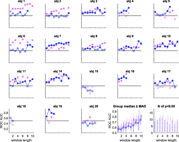
Figure 4. Performance (ROC AUC) of the sLDA whose output was averaged over sequential trials in sliding windows. Individual ROC AUC (for 18 participants, sbj 1 to 20) are shown only if computed over at least 25 windows per class. The last two plots present the same results aggregated over the group. Blue circles are for SMB vs. CT, purple squares are for SSB vs. CT. Filed circles and squares in the individual plots indicate that ROC AUC was higher than random, according to the permutation test (p-values were not corrected for multiple tests).
Download figure:
Standard image High-resolution image3.6. Sensitivity analysis and possible eye movement contribution to the classification
Figure 5 (left) presents plots which show the spatiotemporal distribution of class discriminative information, represented by group medians of individually computed signed  computed between the EEG features used for classification and similarly preprocessed EOG amplitudes, on one hand, and sLDA class probability, on the other hand. From this analysis, we excluded the data of participants 15, 18, and 20, for whom classification was incorrect for both pairs of classes even when trial averaging was used (see figure 4).
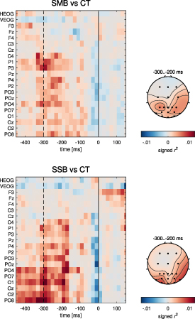
Figure 5. (Left) Spatial-temporal distribution of signed  values (group medians) computed between the EEG/EOG amplitudes and class probability estimated by the sLDA, for classification of voluntary pursuit (SMB) and dwell (SSB) vs. spontaneous pursuit in the counting task (CT). Time is shown relative to the selection triggering. Positive values mean that the probability of classification as the voluntary pursuit (SMB) or dwell (SSB) rather than the spontaneous pursuit in the CT was the higher the more positive was the EEG amplitude. Note that features fed to the classifier were extracted from −300.0 ms interval (marked with dashed and solid vertical lines), and mean over −100.0 ms also served as the baseline. Features from the EOG channels were note used for classification. (Right) Topographical maps of signed
  averaged over the time interval −300 to −200 ms.
Download figure:
Standard image High-resolution image
In the temporal domain, signed  was lower in the time interval used for the baseline in the feature extraction procedure (−100.0 ms), and to the right from it (from where the features were not extracted). Negative values were mainly observed between −40 ms and 0 ms relative to the selection triggering. The highest
  values were found in the EEG channels between −300 ms and −200 ms, and just before this interval (note that the features were taken only from −300.0 ms interval). This pattern suggested that the EEG amplitude change between −300 ms and 0 ms contributed most strongly to the classifier output.
The  values were averaged in −300 to −200 ms interval to create topographical maps (figure 5, right). The maps partly resembled the amplitude maps (figure 3(b)), however, the maxima were not at POz but at other temporal (SMB vs. CT) and occipital (SSB vs. CT) locations. The
  values in the EOG channels were lower than in most EEG channels. Frontal EEG channels turned out to be least informative for the classifier, thus the correlation between the EOG and the classifier output unlikely corresponded to any contribution from EOG artifacts to classification (the correlation could arise from EOG distortion by the ICA-based cleaning procedure).
Finally, we checked if the classifier performance in the case of SMB vs. CT classification would deteriorate when the frontal channels (F3, Fz, F4) were excluded from the classification. ROC AUC insignificantly decreased from 0.58 ± 0.06 to 0.57 ± 0.04 for ICA-cleaned data (median ± MAD; p = 0.88, Wilcoxon matched pairs test) and insignificantly increased for non-ICA-cleaned data, from 0.57 ± 0.04 to 0.58 ± 0.06 (p = 0.40, same test).
4. Discussion
4.1. General remarks
Given that only a limited range of EEG phenomena is available for the use in non-invasive BCIs, it is surprising that the E-wave, the component related to anticipation (expectation), proposed for the use in BCIs in one of the earliest proposals (Walter 1966), has so far attracted almost no attention from the community of BCI developers. The results of this study add to a yet small body of evidence suggesting its usefulness for the BCI technology. We demonstrate here that the E-wave can help to discriminate smooth pursuit eye movements voluntarily used to select an item moving on a computer screen from smooth pursuit eye movements which are not related to the intentional (voluntary) selection.
An interesting application of the E-wave detection proposed by Ihme and Zander (2011) and Protzak et al 2013 is a hybrid BCI system in which eye tracking enables relatively fast and precise detection of candidate items for selection and a BCI reveal if the user is intentionally trying to select, rather than gazing at an item for any other reason. In the case of intentional selection, the user is supposed to expect the result of their action, e.g. some visual change of the item. This is a perfect condition for the E-wave development (see Amit et al 2019 for an analysis of anticipation-related EEG activity in fixation-related data not related to gaze-based control). In the original studies Ihme and Zander (2011) and Protzak et al 2013, as well as in the more detailed analysis by Shishkin et al (2016) and online study by Nuzhdin et al (2017), the items were static and the participants used eye dwells for selection. Unlike quite many other attempts to combine gaze-based selection with a motor imagery-based BCI, from Zander et al (2010) to Hou et al (2020), the hybrid BCI based on the E-wave does not require execution of any additional cognitive task to make selections (the user's task is exactly the same as in usual gaze-based interaction). In contrast to a hybrid BCI where gaze-based selection is combined with the BCI based on the steady-state visual evoked potentials (Brennan et al 2020), no stimuli should be added to the visual interface and, more importantly, the E-wave may help to differentiate voluntary fixations on the items to be selected even from the fixations that are related to items that strongly attract attention but are still spontaneous, so that their selection would be an error.
Here, we demonstrated that the E-wave-based hybrid BCI can be extended to the use of a significantly different class of gaze behavior, namely the smooth pursuit eye movements. This class of gaze behavior can be used to select moving items and has several advantages as an interaction technology over the use of gaze dwells/fixations (Pfeuffer et al 2013, Esteves et al 2015).
In this condition, the presence of several moving items at once presents a challenge, as the distraction caused by non-target items may require more cognitive resources to steadily pursuit the target. Nevertheless, the E-wave that arise during the pursuit in the moving selection condition and during gaze dwells in the static condition were remarkably similar, and classification results did not strongly differ. Thus, the study demonstrated a high flexibility and expandability of the approach.
Note that the EEG under smooth pursuit has been very little explored so far; to the best of our knowledge, our study is the first where the lambda wave followed the end of the pre-pursuit saccade was observed. Studies exploring the effects of the smooth pursuit condition on EEG correlates of cognitive task execution are also rare. Thus, it was not possible to predict, from the earlier results, whether the E-wave amplitude in the gaze-based selection task would maintain high under the smooth pursuit.
4.2. Features used by the classier
Classification of intentional and spontaneous gaze behavior in our study was apparently based on features which were sensitive to an EEG negative wave in the posterior areas (figure 5; figure 3(b)), which was similar or identical to the phenomenon observed earlier in the case of selection of static objects with gaze dwells (fixations) and could be identified as the E-wave or the SPN (Shishkin et al 2016). Note that the E-wave is most often studied as a part of the CNV, an EEG phenomenon with a more anterior localization. However, the CNV also includes motor-related components with frontal localization. When the motor response is excluded from experiment design, pure anticipation-related activity is observed, with the fastest growth in the parietal area (Brunia 1988, Van Boxtel and Brunia 1994, Brunia and Van Boxtel 2001, Van Boxtel and Böcker 2004, Brunia et al 2011, Kotani et al 2015).
Several groups of evidence suggest that the classification of intentional and spontaneous pursuit data in this study could not be strongly inflated by the contribution from electrical potentials related to eye movement, i.e. the EOG. First, classification of SMB vs. CT data (voluntary selection vs. arithmetic task, in both conditions EEG epochs were related to smooth pursuit of moving items) was noticeable similar for the EEG cleaned and not cleaned with ICA from eye movement artifacts. Secondly, as figure 5 shows, features from the frontal EEG electrodes, which are most 'contaminated' with the EOG components, has the lowest correlation with the classifier output. A relatively high correlation for the vertical EOG can be also seen in this figure, however, this could be a coincidence, given that the EOG features were not fed to the classifier. Thirdly, removing features related to the frontal electrodes from the feature set led to only slight and insignificant shifts in ROC AUC (by 0.01). Fourthly, we used only features from the pursuit time interval. While it is accompanied by certain EOG dynamics, the longest possible distance during the time interval used for feature extraction could be 3° and in the majority of trials the distance was much lower, so the EOG contribution to EEG could not be strong. Finally, when a static condition (SSB) was classified against a moving condition (CT), between which the eye movement artifacts were expected to be maximally different, performance improved only slightly compared with SMB vs. CT classification (both were moving conditions); this improvement could be attributed to a high difference between these conditions not only in eye movement artifacts but also in other aspects. Taken all the evidence together, it seems highly likely that the classifier mainly exploited the electrical signal of brain origin to differentiate the pursuit related and not related to intentional attempts to select.
4.3. Limitations of this study
This study is an initial attempt to evaluate the usefulness of the anticipation-related component, the E-wave, for enhancing interaction with computers based on smooth pursuit eye movement. A number of its limitations should be overcome in the future studies. Here we list only the most significant limitations that, in our view, should be addressed first:
- (a)The BCI in this study was not implemented in the online mode, where several factors may hinder the classification of voluntary (intentional) and spontaneous gaze behaviors (Nuzhdin et al 2017). One such factor could be degradation of the EEG marker after missing some voluntary selection attempts by the BCI classifier. Misses can be partly compensated by adding a second, longer dwell time threshold (in our case, time threshold for the pursuit) at which selection occurs without the use of the EEG classifier (Protzak et al 2013). Even in this case BCI misses would lead to variations in the selection time, which may affect the EEG marker. For example, in a study by Amit et al (2019) the CNV amplitude was lower when intervals between the warning and imperative stimuli were irregular compared to a fixed-interval condition. If BCI misses could lead to degradation of the EEG marker, this, in turn, would lead to even lower predictability of the selection time, and so on. The strength of this effect may significantly depend on various factors, thus only online studies may help to judge the feasibility of the hybrid interface. However, unlike in the study of the interaction with a static interface (Nuzhdin et al 2017), here we also consider the possible use of the E-wave-based BCI as a passive system that monitors the degree of the user's involvement into gaze interaction. This possibility should be yet explored in the future studies, but, at least, it seems unlikely that factors specific to online hybrid BCI use, such as described above, will influence the performance in this case.
- (b)Another shortcoming related to the absence of online tests is that conditions that modeled spontaneous pursuit could not be intermixed with voluntary selection conditions but were presented in separate blocks. Moreover, pursuit did not lead to the feedback signals in these conditions, so it is not fully impossible that the participants in these conditions behaved differently from what could be in the online mode, where they had to receive the feedback from time to time. It is not clear how the averaging would work if the moving window cover trials from both classes. Again, online tests will help to resolve these uncertainties. Mixing trials from different conditions could be done even in the offline analysis, however, we refrained from diving into such details, because the results may significantly depend on the classifier (which was unlikely optimal in this study) and other factors.
- (c)The main spontaneous condition (CT) involved perceptual and arithmetic tasks, which could cause event-related (phase-locked) or induced (non-phase-locked) activity in the EEG. However, as can be seen in figure 3, no significant event-related activity arose in this condition. On the other hand, the feature extraction procedure and the linear classifier used in the study could not provide classification based on the non-phase-locked activity. Note that the visual stimuli were absolutely the same in the voluntary and spontaneous conditions before the time of feedback (except for a single static condition), only the instruction was different.In our preliminary studies in small groups of participants who selected moving objects with their gaze (Zhao et al 2018a, 2018b) we found it difficult to find an appropriate control condition, in which moving objects are often enough pursued but without expectation for any upcoming event. Moreover, when the participants were instructed just to pursue a moving object for a certain time without any other task, a similar negative wave was also developed, likely related to anticipation of the time when the pursuit should be canceled. In the current study, pursuit under the instruction to look for a faster ball (FA) also evoked a similar EEG dynamics (figure 3, red dashed lines), which could be related to waiting for a good opportunity to compare the speed of the pursued ball with the speed of some other ball(s) (a strategy often used by the participants). Surprisingly, even the condition less loaded with anticipation, the CT (counting the dots on the moving balls and adding up the number of the ball to the previous sum), was accompanied by a similar deviation of the averaged EEG in some participants. Thus, cautions are due concerning the specific relation of the marker to intentional selection. Nevertheless, in the majority of participants and in the grand average (figure 3) the difference between the intentional selection and this control condition was clear.)In the spontaneous condition FA participants had to announce the number of the ball that they thought was accelerated. To make the analysis more objective and to avoid speech-related artifacts, the announcement could be replaced with the gaze coordinates analysis determining if the pupil movements matched a particular ball. However, this was not possible in our study due to the limitation of the eye tracker license. Also, sometimes a participant initially suspected one ball, but eventually chose another (as they reported after completing the experimental block). A typical case for this situation was when the suspected ball collided with the accelerated ball, and it was the collision of the suspected with the accelerated one that attracted attention to the last one.
- (d)While we used a consumer-grade eye tracker, the experiment procedure did not fully model a practical use case, as we also used a chin rest, a head rest, and a laboratory EEG system. We expected that head stabilization would help to avoid frequent recalibration of the eye tracker and to record a high-quality EEG signal without active electrodes. In a practical situation, head stabilization is often undesirable, but without it, the eye tracking performance could be worse than we observed. However, eye tracking technology is quickly developing, so it seems likely that performance comparable to our results or better will be soon achievable by the consumer-grade eye trackers without any head stabilization. Also, due to the continuing progress in the EEG recording technology affordable and robust to movement EEG systems with dry electrodes are likely to appear soon. Thus, we hope that the experiment setup provides a reasonable approximation of a near-future technology.
- (e)Although we extracted features for the classifier from a time interval preceding the feedback, to simulate an online application where the classifier has to make a decision prior to this time point, we could not fully reproduce the timing in the online mode if the same eye tracker and processing pipeline were used. Indeed, in the offline processing we shifted the trigger generated by the smooth pursuit detection algorithm to compensate for the 140 ms delay. The delay was specific to the low-cost eye tracker we used in this study, while it is not intrinsic to the eye tracker technology in general. Moreover, the delay is not a problem at all if the averaging over trials is used to get a general estimate of the user's involvement in the gaze interaction. Nevertheless, efforts should be made to make the delay shorter in online studies and in possible applications in the case that the E-wave is exploited for on-the-fly differentiation of voluntary and spontaneous gaze dwells on sensitive screen items.
4.4. Prospects
We consider joint use of gaze-related features and the EEG features as a possible way to significantly improve the accuracy of the gaze-based human–computer interfaces (or, in a wider sense, human–machine interfaces). In the current study, this possibility was not explored due to the limitation of the eye tracker license, which did not allow for storing the gaze coordinates and their offline analysis. However, the fusion of the gaze and brain activity information in further studies seems to be very prospective. Improvement of the performance also could be obtained with the use of more advanced classifiers (Kozyrskiy et al 2018), which was difficult to do in this study due to limited dataset sizes. Another important way to improve the accuracy could be creating better conditions for the development of anticipation-related activity in the EEG (e.g. Tecce et al 1976, Linssen et al 2013). One aspect which could negatively influence the E-wave amplitude in our study was a fast rate of selection. In our experiment, participants made selections sequentially and could try to make the intervals between selections as short as possible, so that they could quickly complete the task. Moreover, the time of pursuit before the selection was also short, far below the durations of the interval between the warning and imperative stimuli typically used in the experiments with SPN/E-wave and CNV. It is possible that the use of the interface at a slower pace or for rare actions could be more effective.
Another possible way of classification performance improvement is the averaging of sequential trials. This approach was applied in this study and an improvement was indeed observed (figure 4), although it should be yet tested more rigorously in the future studies, were more trials should be collected and used for classifier training and testing. Of course, it cannot be used for the enhancement of on-the-fly gaze-based selection, but some passive BCI applications operating over longer time scales probably could be developed. For example, if eye tracking is used to select items in a game, the classifier output averaged over sequential trials could be used to estimate the degree of the involvement of the player, and to adjust the game settings accordingly. Sensitivity of the E-wave to perceived control (Mühlberger et al 2017) provides an interesting opportunity to online assess operator's feeling of agency during a human-machine interaction.
Since in this case immediate response of the system is not required, features collected during and after selection-related feedback can be added to the feature vector and possibly further improve the classification. The extended time interval from which features are extracted could even include the P300 wave which we observe in our data after the feedback to intentionally (but not spontaneously) selected items. It is important to consider that the E-wave and the P300 wave are related to significantly different cognitive processes, nevertheless, it is possible that they can be used jointly to index the degree of the involvement into gaze-based interaction.
We discussed above two possible applications of the findings: (a) on-the-fly EEG-based confirmation for the voluntary selection of a pursued moving item, and (b) estimation of the intensity of anticipation of the feedback in gaze interaction based on the smooth pursuit, e.g. for measuring the involvement into interaction. The latter possibility could be considered as a part of a general framework of using gaze-related EEG activity for improving human-machine interaction (Wobrock et al 2020). The range of the E-wave-based applications in gaze interaction, based on either pursuit or dwells, possibly could be even wider. For example, anticipation is considered as an important component of social interaction (Riechelmann et al 2019), this the E-wave, as being related to anticipation, may be considered for estimating the intensity of components of communication, e.g. in systems serving for facilitating remote video communication through the internet.
5. Conclusion
The results suggest the possible usefulness of the EEG E-wave detection in the gaze-based selection of moving items, e.g. in video games. This technique might be more effective when trial data can be averaged, thus it might be more prospective for passive interfaces, for example, used for estimating the degree of the user's involvement during gaze-based interaction.
Acknowledgments
This study was supported in part by the Russian Science Foundation, Grant 18-19-00593 (development of the general approach; elaboration of the selection algorithms; adaptation of techniques for data preprocessing and classification).
The authors thank Alexei E Ossadtchi and the reviewers for useful suggestions.