Abstract
Multi-conjugate adaptive optics (MCAO), consisting of several deformable mirrors (DMs), can significantly increase the adaptive optics (AO) correction field of view. Current MCAO can be realized by either star-oriented or layer-oriented approaches. For solar AO, ground-layer adaptive optics (GLAO) can be viewed as an extreme case of layer-oriented MCAO in which the DM is conjugated to the ground, while solar tomography adaptive optics (TAO) that we proposed recently can be viewed as star-oriented MCAO with only one DM. Solar GLAO and TAO use the same hardware as conventional solar AO, and therefore it will be important to see which method can deliver better performance. In this article, we compare the performance of solar GLAO and TAO by using end-to-end numerical simulation software. Numerical simulations of TAO and GLAO with different numbers of guide stars are conducted. Our results show that TAO and GLAO produce the same performance if the DM is conjugated to the ground, but TAO can only generate better performance when the DM is conjugated to the best height. This result has important application in existing one-DM solar AO systems.
Export citation and abstract BibTeX RIS
1. Introduction
Imaging through a ground-based telescope is severely degraded by turbulence in the Earthʼs atmosphere. Over the past few decades, solar adaptive optics (AO) systems have been deployed at major ground based telescopes, which enable diffraction limited observations of the Sun for a significant fraction of the available telescope observing time (Rimmele 2000, 2004). However, a major limitation of conventional AO is that it can only correct aberrations within a small field of view (FOV) defined by the isoplanatic patch, and the Strehl ratio (SR) will decrease rapidly when the FOV is larger than the isoplanatic angle, which is on the order of a few arcseconds in the visible. Solar activities occur in a two-dimensional extended FOV and studies of solar magnetic fields need high-resolution imaging over an FOV of at least  (Ren et al. 2014; Babcock 1953). Multi-conjugate adaptive optics (MCAO) (Ellerbroek et al. 2003) is a solution to increase the AO corrected FOV, in which several guide stars (GSs) and deformable mirrors (DMs) are used to correct the atmospheric turbulence at different altitudes. In MCAO, the three-dimensional turbulence profile can be found by a tomographic wavefront reconstruction algorithm through phase distortion measurements from multiple GSs located at different field positions (Fusco et al. 1999; Berkefeld & Soltau 2010). There are two different types of MCAOs that may be applied for astronomical high-resolution imaging. One is the star-oriented approach and the other is the layer-oriented approach (Ragazzoni et al. 2000; Nicolle et al. 2006; Rimmele et al. 2010). Star-oriented MCAO uses a tomographic wavefront reconstruction algorithm to find the optimal control signal for each DM. In layer-oriented MCAO, wavefront sensors (WFSs) conjugated to different altitudes directly measure the wavefront at the corresponding altitude from the GSs and the average wavefront is used to control the DM that is optically conjugated to the same height (Glindemann et al. 2000; Arcidiacono et al. 2004, 2010; Vérinaud et al. 2003). Although MCAO is a promising technique for high-resolution imaging over a large FOV, it still is a challenging technique to implement for a solar telescope because of the complexity involved in real-time wavefront measurements and as a result no solar MCAO is available for routine operation.
Traditional solar AO uses an extended field guide region on the order of  for wavefront sensing (Rimmele 2000) and is a typical ground-layer adaptive optics (GLAO) system. Recently, we successfully extended the wavefront sensing FOV up to
  , which efficiently provides a large corrected high-resolution imaging FOV (Ren et al. 2015). We further proposed a solar tomography adaptive optics (TAO) (Ren et al. 2014) system that uses one WFS and one DM. Current solar AO systems use a Shack-Hartmann wavefront sensor (SH-WFS). For both solar GLAO and TAO, the SH-WFS must be conjugated to the ground (i.e. telescope aperture) because of possible vignetting (Ren et al. 2015; Marino & Wöger 2014). Since most turbulence is concentrated on the ground during daytime solar observations, a GLAO or a TAO should be able to deliver good performance over a large corrected FOV, and indeed our recent work demonstrated that both solar GLAO and TAO can generate such good performance in near infrared (NIR) over a large corrected FOV up to
  (Ren et al. 2015).
To compare the performances of the star-oriented and layer-oriented MCAOs, Diolaiti et al. (2001) presented a simplified analytical approach in which only one DM is used. This one-DM comparison can provide insight into the MCAO that uses several DMs. They concluded that the layer-oriented approach is optimal under certain assumptions, and thus both star-oriented and layer-oriented MCAOs should deliver similar performance. According to our knowledge, no numerical simulation work has been conducted. Compared with the analytical approach, numerical simulation comparisons can provide more details such as the number of GSs and asterism configurations which should affect the performance. In this article, we will present numerical simulation comparisons between solar TAO and GLAO in the NIR J band.
In section 2 we present a brief introduction for the solar GLAO and TAO. In section 3, we compare the solar GLAO and TAO performances. In the first case, the DM for both GLAO and TAO is located at the pupil, while in the second case the DM in the TAO is located at the best conjugated height. Finally, we provide our discussion and conclusions of this work.
2. Solar TAO and GLAO Systems
Traditional solar AO relies on an SH-WFS to measure the slope in each subaperture. Since only one GS is used, it cannot reconstruct the wavefront profile. In the TAO we propose, the tomographic wavefront can be measured and reconstructed by using an SH-WFS with multiple GSs (Ren et al. 2014) and thus the reconstructed global wavefront profile information can be applied to control the DM.
Solar GLAO can be done by using several discrete GSs, and all wavefronts measured by an SH-WFS from these discrete GSs are averaged (Ren et al. 2015). The averaged wavefront is corrected by a DM conjugated to the telescope aperture. For a linear system, this approach is equivalent to getting all the slopes in each subaperture from these discrete GSs and then calculating the average slope that is used to control the DM. Solar GLAO corrects the wavefront errors induced by ground-layer turbulence and leaves the wavefront error induced by high altitude turbulence uncorrected because of the implementation of a DM conjugated to the ground without tomographic reconstruction. GLAO can be considered as a kind of one-DM layer-oriented MCAO. Star-oriented and layer-oriented MCAOs are also studied with analytical expressions by Nicolle et al. (2004). However, their research is focused on how the GS brightness affects the MCAO performance, which is not a concern for solar wavefront sensing, since enough photons are available.
To make the performance comparisons fair, the same number of GSs, asterism configuration and WFS should be used. It is also important to run the same simulation software, which can avoid software to software discrepancies in the performance simulations. In our previous work, we have considered the performances of both solar TAO and GLAO. However, they are calculated with different software tools and different GS numbers and asterisms. Here we use identical GSs and software to compare the performances of solar GLAO and TAO. The software we used for the performance calculations is YAO (Rigaut1a & Van Dam 2013), which is an end-to-end Monte-Carlo AO simulation software tool. Its open source codes allow users to further develop the codes for specific applications. For our solar TAO, we can directly use YAOʼs star-oriented MCAO. For solar GLAO, the average slope from all the GSs is calculated first, and then the average value is used to feed a standard AO loop for the performance simulations.
3. Solar TAO and GLAO Simulations
For solar TAO and GLAO performance simulations, we use the Big Bear Solar Observatory (BBSO) site seeing measurement data, which represent the only available seeing profile at a major solar site and were discussed recently by Kellerer (Kellerer et al. 2012). The BBSO seeing data show that most of the turbulence is concentrated in four layers.
Table 1 displays the Fried parameter r0 at different heights above the telescope aperture as well as the layer fraction  , which defines how much turbulence is concentrated in each layer. The layer fraction at layer i can be calculated as
where the overall seeing parameter r0total = 0.096 m, which is a typical value at a good seeing condition and is most suitable for solar high-resolution imaging. We assume that the solar TAO and GLAO work at  J band with a 1.6-m aperture telescope, which is the largest solar telescope currently available. We use an SH-WFS with 10 × 10 subapertures to measure the wavefront. No readout noise is considered, since enough photons are available for solar wavefront sensing. For each calculation, we use the data generated from 1000 close-loop iterations to evaluate the average SR at each position in the FOV.
Table 1. Seeing Parameter r0 at Different Heights by BBSO Site Data
| Height (m) | 200 | 1000 | 3000 | 8000 |
|---|---|---|---|---|
| r0 (m) | 0.125 | 0.230 | 0.420 | 0.700 |
| Layer fraction | 0.644 | 0.234 | 0.085 | 0.037 |
In order to calculate the performances in an extended imaging FOV, imaging FOV up to  is used. The numbers of GSs 4, 9 and 13 are used, with the asterisms shown in Figure 1, in which one GS is located at the center of the wavefront sensing field and the others are located symmetrically in the field. Two FOVs are defined. The OFOV is defined as the FOV for wavefront sensing and is the field that needs to be optimized, while the imaging FOV is the field used to evaluate the imaging performance. For solar TAO and GLAO evaluations, we use a large OFOV of
  and
and  in diameter respectively.
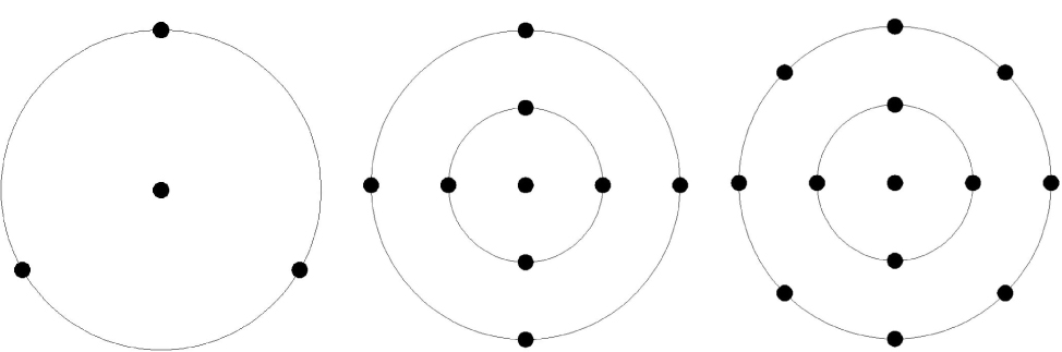
Fig. 1 Asterism with four GSs (left), nine GSs (center) and 13 GSs (right) in the OFOV.
Download figure:
Standard image3.1. DM Conjugated to the Telescope Aperture
In this case, both DMs for GLAO and TAO are located at the telescope pupil. That is, the DM conjugated height is zero for both GLAO and TAO. Table 2 shows the results of simulations with the BBSO seeing profile of the solar TAO and GLAO conjugated to the telescope aperture when four GSs are used. The result shows that solar TAO delivers slightly better performance in the imaging FOV between  , with an SR between
  for
for  OFOV, respectively. Solar GLAO provides good performance in the imaging FOV between
  , with an SR between
  for
for  OFOV, respectively. The comparisons of solar TAO and solar GLAO are also presented in Figure 2.
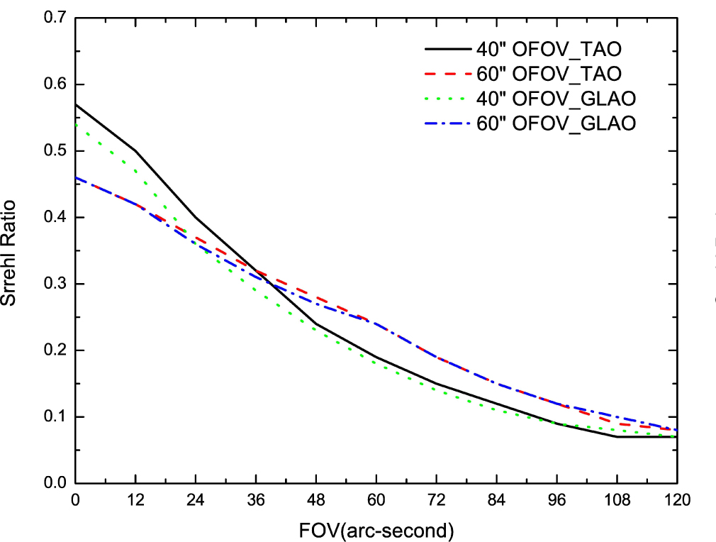
Fig. 2 SRs as a function of imaging FOV for the TAO and GLAO conjugated to the telescope aperture with four GSs at the NIR J band.
Download figure:
Standard imageTable 2. SRs of TAO and GLAO with Four GSs
| Imaging FOV |

|

|

|

|

|

|

|

|

|

|

|
|---|---|---|---|---|---|---|---|---|---|---|---|
 OFOV_TAO OFOV_TAO |
0.57 | 0.50 | 0.40 | 0.32 | 0.24 | 0.19 | 0.15 | 0.12 | 0.09 | 0.07 | 0.07 |
 OFOV_TAO OFOV_TAO |
0.46 | 0.42 | 0.37 | 0.32 | 0.28 | 0.24 | 0.19 | 0.15 | 0.12 | 0.09 | 0.08 |
 OFOV_GLAO OFOV_GLAO |
0.54 | 0.47 | 0.36 | 0.29 | 0.23 | 0.18 | 0.14 | 0.11 | 0.09 | 0.08 | 0.07 |
 OFOV_GLAO OFOV_GLAO |
0.46 | 0.42 | 0.36 | 0.31 | 0.27 | 0.24 | 0.19 | 0.15 | 0.12 | 0.10 | 0.08 |
It is clear that both solar TAO and GLAO can generate good performance over a large FOV, as shown in Figure 2. While the TAO performs slightly better than GLAO, the difference is very small for the 4-GS case.
Increasing the number of GSs can improve wavefront measurement accuracy over a large FOV and thus improve the performances for both systems. Table 3 lists the results of SRs for TAO and GLAO with nine GSs, in which the DMs are conjugated to the telescope aperture. From Table 3, solar TAO delivers slightly better performance in the imaging FOV between  , with an SR between
  for
for  OFOV, respectively. Solar GLAO yields good performance in the imaging FOV between
  , with an SR between
  for
for  OFOV, respectively. Both solar TAO and GLAO stably provide better performance over the large OFOV with nine GSs than that with four GSs. The comparisons of TAO and GLAO are also presented in Figure 3.
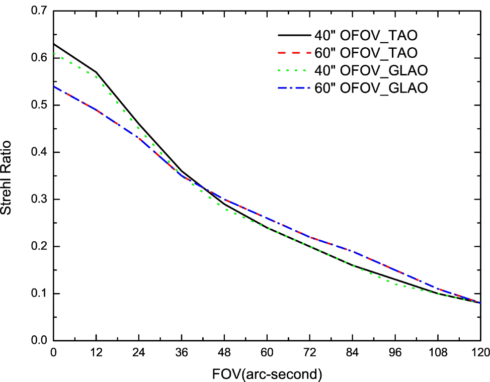
Fig. 3 SRs of TAO and GLAO conjugated to the telescope aperture with nine GSs at the NIR J band.
Download figure:
Standard imageTable 3. SRs of TAO and GLAO with Nine GSs
| Imaging FOV |

|

|

|

|

|

|

|

|

|

|

|
|---|---|---|---|---|---|---|---|---|---|---|---|
 OFOV_TAO OFOV_TAO |
0.63 | 0.57 | 0.46 | 0.36 | 0.29 | 0.24 | 0.20 | 0.16 | 0.13 | 0.10 | 0.08 |
 OFOV_TAO OFOV_TAO |
0.54 | 0.49 | 0.43 | 0.35 | 0.30 | 0.26 | 0.22 | 0.19 | 0.15 | 0.11 | 0.08 |
 OFOV_GLAO OFOV_GLAO |
0.61 | 0.56 | 0.45 | 0.35 | 0.28 | 0.24 | 0.20 | 0.16 | 0.12 | 0.10 | 0.08 |
 OFOV_GLAO OFOV_GLAO |
0.54 | 0.49 | 0.43 | 0.35 | 0.30 | 0.26 | 0.22 | 0.19 | 0.15 | 0.11 | 0.08 |
We continue to increase the number of GSs to 13. Table 4 presents the results of SRs for the solar TAO and GLAO with 13 GSs. From Table 4, solar TAO delivers good performance in the imaging FOV between  , with an SR between
  for
for  OFOV, respectively. Now, solar GLAO generates identical performance as TAO. That is, solar TAO provides the same performance as GLAO over the whole imaging FOV. The comparisons between solar TAO and GLAO are also shown in Figure 4, which clearly indicates that GLAO and TAO will deliver identical performance by using a large number of GSs.
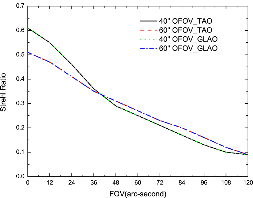
Fig. 4 SRs of the TAO and GLAO conjugated to the telescope aperture with 13 GSs at the NIR J band.
Download figure:
Standard imageTable 4. SRs of TAO and GLAO with 13 GSs
| Imaging FOV |

|

|

|

|

|

|

|

|

|

|

|
|---|---|---|---|---|---|---|---|---|---|---|---|
 OFOV_TAO OFOV_TAO |
0.61 | 0.55 | 0.46 | 0.36 | 0.29 | 0.25 | 0.21 | 0.17 | 0.13 | 0.10 | 0.09 |
 OFOV_TAO OFOV_TAO |
0.51 | 0.47 | 0.41 | 0.35 | 0.31 | 0.27 | 0.23 | 0.20 | 0.16 | 0.12 | 0.09 |
 OFOV_GLAO OFOV_GLAO |
0.61 | 0.55 | 0.46 | 0.36 | 0.29 | 0.25 | 0.21 | 0.17 | 0.13 | 0.10 | 0.09 |
 OFOV_GLAO OFOV_GLAO |
0.51 | 0.47 | 0.41 | 0.35 | 0.31 | 0.27 | 0.23 | 0.20 | 0.16 | 0.12 | 0.09 |
3.2. TAO with DM Located at the Best Conjugated Height
While solar GLAO with both WFS and DM conjugated to the telescope pupil can only measure and correct the ground layer turbulence, solar TAO can fully take advantage of the three-dimensional tomographic wavefront information, which can be reconstructed from measurements of multiple GSs, and the DM can be conjugated to the best conjugated height to provide the best performance over a large FOV. The best DM conjugated height can be calculated analytically with the mean turbulence height H as defined in Equation (2), which can be viewed as equivalent to the height for only one layer (Hardy 1998).
where  is the atmospheric structure constant at different heights h. In general, the mean turbulence height can be calculated from the above equation and it is in good agreement with the best conjugated height found by numerical simulations (Ren et al. 2014). Although the best conjugated height can be calculated with the mean turbulence height, it is straightforward to find by using different conjugated heights in numerical simulations. This means that the performance of TAO can be further improved by moving the DM to the best-conjugated height, where most turbulence is located.
Figure 5 shows the numerical simulation results of the on-axis SR, which are calculated on the OFOV of  with four GSs. From Figure 5, it is found that the best conjugated height is 900 m. At the best conjugated height, SRs in other positions in the OFOV are also improved. However, the on-axis value has the most significant change and is thus used to find the best conjugated height.
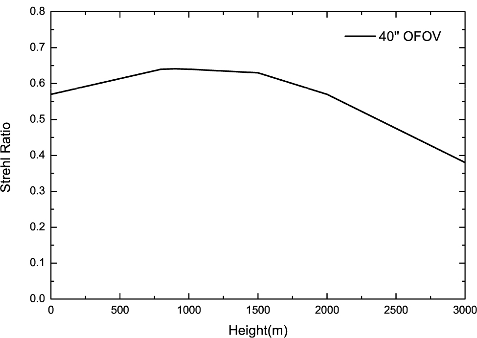
Fig. 5 On axis SR as a function of DM conjugated height. The SR is calculated for  OFOV.
OFOV.
Download figure:
Standard imageTable 5 presents the SRs of TAO at the 900 m best conjugated height and the GLAO conjugated to the telescope aperture with four GSs at  in J band. From the table, solar TAO delivers better performance in the imaging FOV between
  , with an SR between
  for
for  OFOV, respectively. Solar GLAO yields good performance in the imaging FOV between
  , with an SR between
  for
for  OFOV, respectively. The comparisons are also shown in Figure 6. It is clear that by fully taking advantage of the tomographic wavefront information, solar TAO can achieve a significant performance gain.
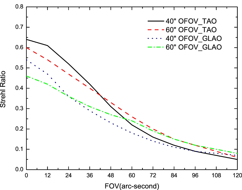
Fig. 6 SRs of TAO conjugated at a height of 900 m and GLAO conjugated to the telescope aperture at the NIR J band with four GSs.
Download figure:
Standard imageTable 5. SRs of TAO at the Best Conjugated Height and GLAO Conjugated to the Telescope Aperture with four GSs
| Imaging FOV |

|

|

|

|

|

|

|

|

|

|

|
|---|---|---|---|---|---|---|---|---|---|---|---|
 OFOV_TAO OFOV_TAO |
0.64 | 0.61 | 0.52 | 0.42 | 0.31 | 0.22 | 0.16 | 0.12 | 0.09 | 0.07 | 0.05 |
 OFOV_TAO OFOV_TAO |
0.60 | 0.54 | 0.47 | 0.40 | 0.33 | 0.26 | 0.20 | 0.15 | 0.12 | 0.09 | 0.06 |
 OFOV_GLAO OFOV_GLAO |
0.54 | 0.47 | 0.36 | 0.29 | 0.23 | 0.18 | 0.14 | 0.11 | 0.09 | 0.08 | 0.07 |
 OFOV_GLAO OFOV_GLAO |
0.46 | 0.42 | 0.36 | 0.31 | 0.27 | 0.24 | 0.19 | 0.15 | 0.12 | 0.10 | 0.08 |
The TAO performance can be further improved by increasing the number of GSs. Table 6 presents the results of SRs for TAO and GLAO with nine GSs. Again, the DM for TAO is conjugated at the best conjugated height of 900 m, while the DM for GLAO is conjugated at the telescope aperture with zero conjugated height. From Table 6, solar TAO delivers better performance in the imaging FOV between  , with an SR between
  for
for  OFOV, respectively. The GLAO provides good performance in the imaging FOV between
  , with an SR between
  for
for  OFOV, respectively. The comparison of solar TAO and GLAO is also shown in Figure 7. Comparing table 5 and Table 6, both TAO and GLAO yield better performance with nine GSs than with four GSs, and in general, TAOʼs performance is better than that of GLAO.
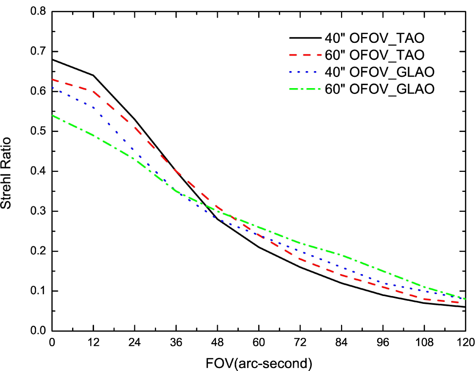
Fig. 7 SRs of TAO conjugated at a height of 900 m and GLAO conjugated to the telescope aperture in the NIR J band with nine GSs.
Download figure:
Standard imageTable 6. SRs of TAO at the Best Conjugated Height and GLAO Conjugated to the Telescope Aperture with four GSs based on Theoretical Seeing Profile
| Imaging FOV |

|

|

|

|

|

|

|

|

|

|

|
|---|---|---|---|---|---|---|---|---|---|---|---|
 OFOV_TAO OFOV_TAO |
0.68 | 0.64 | 0.53 | 0.40 | 0.28 | 0.21 | 0.16 | 0.12 | 0.09 | 0.07 | 0.06 |
 OFOV_TAO OFOV_TAO |
0.63 | 0.60 | 0.51 | 0.40 | 0.31 | 0.24 | 0.18 | 0.14 | 0.11 | 0.08 | 0.07 |
 OFOV_GLAO OFOV_GLAO |
0.61 | 0.56 | 0.45 | 0.35 | 0.28 | 0.24 | 0.20 | 0.16 | 0.12 | 0.10 | 0.08 |
 OFOV_GLAO OFOV_GLAO |
0.54 | 0.49 | 0.43 | 0.35 | 0.30 | 0.26 | 0.22 | 0.19 | 0.15 | 0.11 | 0.08 |
3.3. Simulations with Theoretical Seeing Profile
Until now, all our simulations have been based on BBSO seeing data. It will be valuable to see the result for the seeing profile in a general case, for which we use the theoretical equation recommended by the ATST/DKIST site survey team. The equation to calculate theoretical daytime seeing profiles at height h above the telescope aperture is (Hill et al. 2003),

where the first part on the right of the equation is the Hufnagel-Valley model for a typical nighttime turbulence profile of mountain sites, and the second part indicates the extra turbulence induced by the daytime ground boundary layer. AB is the boundary amplitude and h0 is the boundary scale height. As shown in Table 7, the theoretical daytime seeing profile with 10 discrete layers is calculated according to Equation (3), while the overall Fried parameter is equal to 7.0 cm and the site altitude above sea level is 3000 m. Such a profile can represent the typical daytime seeing distribution for most high altitude solar sites such as BBSO, Sacaramento Peak, La Palma and Haleakala, and was used for simulations of solar TAO in our previous paper (Ren et al. 2014).
Table 7. Seeing Parameter r0 at Different Heights by Theoretical Modeling
| Height (m) | 200 | 700 | 1500 | 2500 | 4000 | 6000 | 8000 | 10000 | 12000 | 14000 |
|---|---|---|---|---|---|---|---|---|---|---|
| r0 (m) | 0.110 | 0.140 | 0.210 | 0.530 | 1.04 | 1.90 | 2.01 | 2.45 | 3.42 | 5.33 |
| Layer fraction | 0.469 | 0.314 | 0.159 | 0.034 | 0.011 | 0.004 | 0.004 | 0.003 | 0.001 | 0.001 |
Comparing the seeing profiles of Table 1 and Table 7, the turbulence of the ground layer (0–500 m) and extended ground layer (1–2 km) dominates the seeing profile distribution, in which more than 80% of the layer fractions are concentrated at heights below 3000 m for both BBSO and the theoretical seeing profiles. We did the solar TAO and GLAO simulations based on the theoretical seeing profile in Table 7 and obtained similar results with the simulations based on BBSO data, which indicate our results described in Sections 3.1 and 3.2 can also be applied to other seeing conditions.
4. Discussion and Conclusions
The performances of solar TAO and GLAO are discussed with different GS numbers. When the DM is conjugated to the ground with a small number of GSs, such as 4 or 9, solar TAO can deliver slightly better performance than GLAO. Increasing the number of GSs to a large number, such as 13, for both TAO and GLAO will yield identical performance. While our end-to-end numerical simulation results give more details at different conditions such as GS number and geometrical configurations, our results are, in fact, consistent with the analytical results derived by Diolaiti et al. (2001), who stated that both star-oriented MCAO and layer-oriented MCAO generate similar performances in ideal conditions (i.e. high density GSs and each GS is viewed as an ideal delta function). The results we found here can also be applied to the layer-oriented and star-oriented MCAOs.
Depending on the seeing profile distribution, conjugating the DM to the best conjugated height in the TAO can provide a significant performance gain, which results in performance that is superior to GLAO, since TAO can fully take advantage of global tomographic wavefront information and the DM can be moved away from the pupil to the best conjugated height. This result has important applications to solar wide-field high-resolution imaging, and it will allow current conventional solar AO to gain an extra improvement in performance by simply shifting the DM to the best conjugated height in an actual system, from which the tomographic turbulence distributions can be measured by using a portable seeing profiler that we proposed recently (Zhao & Ren 2015; Ren & Zhao 2016). Solar AO uses a small extended guide region on the order of  for slope calculation. Although we implement point GSs for the numerical simulations, our results for the solar GLAO and TAO hold true with those using extended regions as GSs. For solar GLAO and TAO that employ multiple GSs to optimize wide-field high-resolution imaging as we discussed here, using an extended guide region can be viewed as an increase in the number of GSs. That is, each extended guide region can be viewed as a number of GSs whose gap is characterized by the so-called isoplanatic angle. When used in TAO and GLAO, the extra GSs from each extended guide region can be viewed as a number of individual GSs. Since with a large number of GSs, both TAO and GLAO deliver identical performance (of course with DM conjugated to the same height for both systems), this implies that when using extended guide regions, TAO and GLAO are intended to provide identical performance. In fact, increasing the number of GSs will, because of extended guide region, create a more uniform correction in the FOV, which may further improve the performance of GLAO or TAO.
Acknowledgements
D. Ren acknowledges the support of NSF under grant AST-1607921 and a grant from the Mt. Cuba Astronomical Foundation.