


Abstract
Bright six-partite continuous-variable (CV) entanglement generated by the coupled intracavity sum frequency generation is investigated. The entanglement characteristics of reflected pump fields and the output sum frequency fields are discussed theoretically in symmetric and asymmetric cases by applying van Loock and Furusawa criteria for multipartite CV entanglement. Such compact tunable multipartite CV entanglement, generated from an experimentally feasible coupled system, could be used in integrated quantum communication and networks.
Export citation and abstract BibTeX RIS
1. Introduction
Quantum entanglement is the foundation of quantum physics and the key resource of quantum information processing [1]. Over the course of the past few decades, continuous-variable (CV) entanglement, especially multipartite CV entanglement, has drawn much attention in its potential applications in quantum communication and computation, which include quantum-controlled dense coding [2, 3], quantum telecloning [4, 5] and quantum teleportation network [6]. Multipartite CV entanglement fields with different frequencies are more useful in connecting different physical systems at the nodes of quantum networks in contrast to those with the same frequency generated by beam splitters [7, 8]. Many papers have reported the schemes which can generate two-color or multi-color CV entangled beams by an optical parametric down-conversion process [9–13], frequency up-conversion process [14–17] and cascaded or concurrent nonlinear processes [18–29].
In addition, the nonlinear optical coupler consists of two parallel nonlinear optical waveguides, which coupled by evanescent overlaps of the guided modes can generate two-color or multi-color CV entanglement. This type of coupling was theoretically and experimentally investigated decades ago [30, 31]. The coupled degenerate parametric down-conversion can generate bipartite [32–34] or two-color quadripartite CV entanglement [35] in traveling-wave configuration or in an optical cavity. Moreover, the coupled non-degenerate parametric down-conversion in an optical cavity can produce bright three-color six-partite entanglement [36]. Olsen et al studied the Kerr nonlinear coupler that produces bipartite CV entangled beams and can be used to demonstrate the Einstein–Podolsky–Rosen (EPR) paradox [37]. Coupled up-conversion processes, unlike coupled parametric down-conversion processes, can also generate bright multipartite CV entanglement. Since second harmonic generation (SHG) and sum frequency generation (SFG) have no oscillation threshold, the generated entangled fields become macroscopically occupied as soon as the low-frequency (LF) pumping fields are turned on. Bache et al theoretically discussed the coupled SHGs and analyzed the intensity correlations as well as the phase-dependent correlation features [38]. Bright bipartite [39] and two-color quadripartite [40] entanglement can be produced by coupled SHGs inside an optical cavity. The related system is all-integrated, which makes it a compact robust source of CV entanglement.
In this present letter, we proposed a scheme for the generation of bright three-color six-partite CV entanglement from the coupled SFG processes in an optical cavity in which periodically poled LiTaO3 waveguides serve as the gain medium. The periods can be designed flexibly according to the practical application. The quantum correlations among these six output beams and the steady-state regions are analyzed according to the inseparability criterion for multipartite CV entanglement as proposed by van Loock and Furusawa [41].
2. Theory
The proposed scheme, which consists of two parallel adjacent nonlinear waveguides and an optical cavity, is shown in figure 1. The two waveguides are fabricated in a periodically poled quadratic nonlinear optical crystal. Efficient SFG processes take place in each waveguide. These two waveguides are numbered A and B, respectively. M1 and M2 are the coupler mirrors. The linear coupling between these waveguides is achieved by the evanescent wave overlaps of the intracavity guide modes. LF pump fields  (with the frequency of
  ) and
) and  (with the frequency of
  ) are incident upon the nonlinear waveguides A and B through the coupler mirror M1.
  (with the frequency of
  ) are sum frequency (SF) fields in waveguides A and B, respectively. The energy conservation condition is
  . Here, we assume that the two SFG processes are equal and all the modes inside the waveguides are perfectly phase matched using the technique of quasi-phase-matching (QPM). Because the periods can be flexibly designed according to QPM, almost any desired wavelength of the entangled beams can be obtained by modification of the phase-matching conditions and the LF pump wavelengths. For example, we can choose two LF pump field wavelengths as 1560 and 780 nm, respectively. The SF field is centered at 520 nm. 1560 nm is suitable to be transmitted through optical fibers over long distances and 780 nm is one of the absorption lines of the rubidium atom, which is an ideal candidate for the storage in quantum repeater of quantum information.
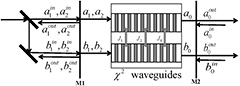
Figure 1. Experimental setup for the proposed scheme.
Download figure:
Standard image High-resolution imageThe effective Hamiltonian for this system can be written as

The interaction Hamiltonian for the coupled system is
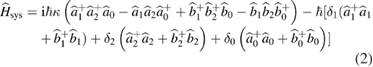
where, the first part of the Hamiltonian stands for the SFG processes, and the second part is the free Hamiltonian of the cavity modes for the LP pump and SF fields.  is the dimensionless nonlinear coupling coefficient of our system, which is proportional to the nonlinear susceptibility and the structure parameters of the periodically poled nonlinear optical waveguides, and taken to be real without loss of generality [9].
  , and
, and  are bosonic annihilation operators for the mode at frequency
  in waveguides A and B, respectively.
  are the cavity detunings from their respective resonances.
The coupling Hamiltonian is described by
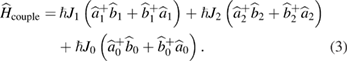
In the above,  are the linear coupling parameters at three different frequencies of two nonlinear waveguides. As [38] described, the lower frequency (
 and
and  ) coupling parameters
  and
and  are larger than the higher frequency (
 ) coupling parameter
  .
.
Finally, the cavity damping can be written as
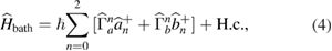
where  and
and  are the bath operators in two waveguides for three different frequencies, respectively.
The quantum Langevin equations of motion for the six intracavity fields according to the input–output formalism developed by Collett and Gardiner [42] can be obtained as
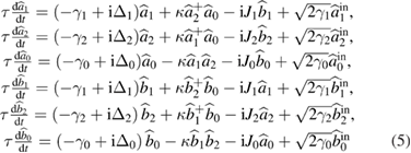
where  is the cavity round-tip time and assumed to be the same for all the cavity modes.
  and
and  are the input field operators of the cavity of two waveguides. The dimensionless variables
 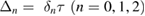 , represent the cavity detunings of the SF and two LF pump fields, respectively.
  are the loss coefficients of the cavity modes, which are related to the amplitude reflection coefficients and the amplitude transmission coefficients.
3. Stationary solutions and quantum fluctuations of the output fields
By setting the left side of equation (5) to be zero and replacing all the operators with their mean values, we can get a set of equations for the classical steady-state values, i.e.
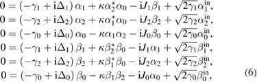
where  and
and  are the steady-state amplitudes of the intracavity modes
  and
and  , respectively. For simplicity, we will make some assumptions: two waveguides are equal and the initial phases of two coherent LF pump fields are to be zero. Therefore, we set
 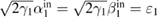 and
and  and no input of the SF fields, i.e.
 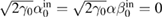 . Also, the steady-state solutions in two waveguides are equal, i.e.
  ,
,  and
and  .
.
In the following, we will discuss this system in the case of detuning the cavity by an appropriate amount from three frequencies so as to simplify the theoretical analysis and actually improve some quantum correlations, i.e.  ,
,  and
and  . Then, we will solve the steady-state equations in two cases, the first symmetric case, where the frequencies of two LF pump fields are close to each other, i.e.
  is close to
  , and we can assume the system parameters of these modes in two waveguides as
  ,
,  ,
,  ,
,  ,
,  and
and  . Therefore, under this assumption, we can get the steady-state solutions for the symmetry case as
with ![$A=\sqrt[3]{-2{{\gamma}^{3}}\gamma _{0}^{3}{{\kappa}^{3}}-27{{\varepsilon}^{2}}{{\kappa}^{5}}\gamma _{0}^{2}+\sqrt{27{{\varepsilon}^{2}}{{\kappa}^{8}}\gamma _{3}^{4}(4{{\gamma}^{3}}{{\gamma}_{0}}+27{{\varepsilon}^{2}}{{\kappa}^{2}})}}$](https://content.cld.iop.org/journals/1612-202X/15/4/045202/revision1/lplaa9fb5ieqn048.gif) .
.
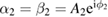
The other asymmetric case, i.e.  ,
,  ,
,  ,
,  ,
,  and
and  . Therefore, the steady-state solutions for the asymmetry case can be written as
with  being the solution of the following high-order equation:

Because equation (9) is a five-order equation, we cannot get its analytical solutions of steady-state equations in the asymmetric case.
In order to analyze the spectral correlations of the output modes, we may linearize the system variables into their classical steady-state solutions and small quantum fluctuations, i.e.  and
and  . Here, we define
  and
and  , as the fluctuations of the amplitude quadrature and
  and
and  stand for the fluctuations of the phase quadrature of each mode. Substituting these expressions into equation (5) and neglecting second- and higher-order terms of the fluctuations, we can obtain the linearized equation for the fluctuations as
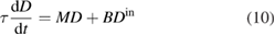
with


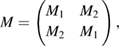
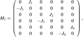
where  ,
,  ,
,  ,
,  ,
,  and
and  .
.
As long as none of the eigenvalues of matrix M develop a positive real part, the fluctuations will not tend to increase exponentially, and the linearized fluctuation analysis is valid. In this present letter, we only study the region where the linearization analysis is valid. Because the analytical eigenvalues of matrix M cannot be obtained, we give the numerical results of the real parts of the eigenvalues. For the symmetry case, the real parts of the eigenvalues of matrix M are schematically shown in figure 2 versus different system parameters  ,
,  ,
,  ,
,  and
and  . In figures 2(a) and (b), we plot the real parts of the eigenvalues versus the loss coefficients
  and
and  with the system parameters chosen as
  ,
,  ,
,  and
and  . Figure 2(c) depicts the dimensionless nonlinear coupling coefficients
  with
with  and
and  . Figures 2(d) and (e) depict the real parts of the eigenvalues versus the symmetric pump power ε and the coupling parameter
  of two LF fields, respectively.

Figure 2. Real parts of the eigenvalues of drift matrix M versus different system parameters  ,
,  ,
,  ,
,  and
and  for the symmetry case.
Download figure:
Standard image High-resolution imageFor the asymmetry case, one can numerically obtain the real parts of the eigenvalues of drift matrix M versus different system parameters  ,
,  ,
,  ,
,  ,
,  ,
,  ,
,  and
and  as shown in figure 3. The parameters used in figures 3(a)–(c) are
  ,
,  ,
,  ,
,  ,
,  and
and  . In figure 3(d), the parameters are chosen as
  ,
,  and
and  , while the other parameters remain unchanged. In figures 3(e)–(h)
  and the rest of the parameters are the same as in figure 3(d).

Figure 3. Real parts of the eigenvalues of drift matrix M versus different system parameters  ,
,  ,
,  ,
,  ,
,  ,
,  ,
,  and
and  for the asymmetry case.
Download figure:
Standard image High-resolution imageFrom figures 2 and 3, one can see that the values of the solid lines, which represent the real parts of the eigenvalues of drift matrix M are all negative in a wide range of all given system parameters, which indicate clearly that the system is stable and the linearization analysis is valid in this region. In this present letter, we only study the region where the linearization analysis is valid.
By using the Fourier transformation and the boundary condition  on the coupler mirror [42], the output fluctuations in the frequency space can be obtained as

where  is the unit matrix.
4. Characteristics of entanglement for the output modes
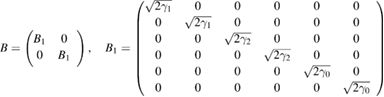
In the following, we will investigate the entanglement characteristics of six output beams of this system by employing the sufficient inseparability criterion for multipartite CV entanglement, which is given by van Loock and Furusawa [41]. In order to sufficiently verify that the six beams of this system are fully inseparable and possess the property of genuine six-partite entanglement, the following five inequalities should be violated at the same time:
In order to study the correlation between two SF fields of two waveguides, we also take the next equation into account:

where  are scaling factors, which can be freely adjusted to minimize the correlation spectra functions.
We will first numerically discuss the quantum correlation spectra in the symmetry case versus different system parameters. Due to the symmetry of two waveguides, we have  and
and  . In figure 4, we plot the quantum correlation spectra versus the analysis frequency
  with
with  ,
,  ,
,  ,
,  ,
,  and
and  , respectively. As shown in this figure, these five inequalities are violated, so we can conclude that genuine six-partite entanglement can be achieved. In addition, the correlations between two LF pump fields are better than those of any other fields, and the best six-partite entanglement is obtained at about
  .
.

Figure 4. Quantum correlation spectra versus the normalized analysis frequency  .
.
Download figure:
Standard image High-resolution imageThe dependence of quantum correlation spectra on LF pump power  is shown in figure 5, where
  ,
,  ,
,  ,
,  ,
,  and
and  , respectively. In this figure, one can see that the values of these five curves are all less than four when
  is greater than 170, which demonstrates that these six modes are entangled. For the given set of parameters, the best six-partite entanglement is achieved around
  . Also, the correlations between the LF pump fields is much better than those of other fields, and the correlations between the generated SF fields are first increased and then decreased as the LF pump fields increase. This characteristic is the same as the uncoupled SFG.
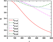
Figure 5. Quantum correlation spectra versus LF pump power  .
.
Download figure:
Standard image High-resolution imageFigure 6 depicts the quantum correlation spectra versus the linear coupling parameter of two LF pump fields  with
with  ,
,  ,
,  ,
,  ,
,  ,
,  and
and  , respectively. As shown in this figure, when the value of
  is very small, i.e. the linear interaction between the two waveguides is small, there is only quantum correlation among the modes of each waveguide, but no correlation between the modes from different waveguides and these six modes are not entangled with each other. With increasing the value of
  and when
  , the values of all the correlation curves are less than four. Continuously increasing the value of
  , one can find that almost all the values of the correlation spectra do not change, which indicates that these six modes are entangled with each other as long as
  .
.
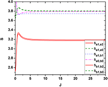
Figure 6. Quantum correlation spectra versus the linear coupling parameter of the down-converted modes  .
.
Download figure:
Standard image High-resolution imageNext, we will discuss the asymmetry case, i.e.  ,
,  ,
,  ,
,  ,
,  and
and  . We plot the quantum correlation spectra versus the analysis frequency
  in figure 7 with
  ,
,  ,
,  ,
,  ,
,  ,
,  ,
,  ,
,  and
and  , respectively. It is obvious that the values of these six quantum correlation spectra are all less than four, and violate six inequalities in equation (12). Therefore, these six output fields are genuine six-partite entanglement in the asymmetrical case. The best correlation can be obtained at
  .
.

Figure 7. Quantum correlation spectra versus the normalized analysis frequency  .
.
Download figure:
Standard image High-resolution imageFigure 8 shows the result of the quantum correlation spectra versus the ratio of two LF pump power  with
with  ,
,  and the other parameters remain unchanged as in figure 7. As shown in this figure, when
  there is no entanglement between any two fields. This might be because the power of pump field
  is much lower than that of
  , and the quantum property of pump field
  is not present in such a case. By increasing the power of pump field
  , the nonlinear conversion efficiency is increased, while pump field
  becomes weaker, and two LF pump fields begin to entangle with each other. With further increasing the power, the quantum properties of these six fields are present and bright three-color six-partite CV entanglement appears when
  . Moreover, the correlation between LF pump fields is always better than that of pump
  and the SF field. The correlation of the fields in the same waveguide is better than that of fields in different waveguides. Compared with other cases, we achieve the largest degree of entanglement when
  .
.
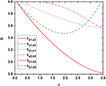
Figure 8. Quantum correlation spectra versus the ratio of two LF pump power  .
.
Download figure:
Standard image High-resolution imageFigure 9 depicts the relationship between the quantum correlation spectra with the linear coupling parameter  . We set
  and
and  and other parameters remain unchanged. From this figure, we can see that the result is similar to figure 6; i.e. when the value of
  is very small, there is no entanglement among the output fields of different waveguides, and it only exists when the quantum correlation is among the fields of the same waveguide. When
  is increased to
  , the values of all the correlation curves are less than four and, six-partite entanglement appears. And as long as
  almost all the values of the correlation spectra do not change.

Figure 9. Quantum correlation spectra versus the linear coupling parameter  .
.
Download figure:
Standard image High-resolution image
5. Conclusions
In conclusion, we proposed a theoretical scheme for producing bright three-color six-partite CV entanglement based on coupled SFG processes. LF pump fields exit the optical cavity from one side, while spatially separated and SF beams exit the optical cavity from the other side. We theoretically analyzed the quantum correlation spectra of six output fields in symmetric and asymmetric cases and found that the entanglement characteristics are influenced by different system parameters. This integrated scheme may have applications in the field of quantum cryptography and quantum communication networks.
Acknowledgments
This research was supported by the NNSFC (grant nos. 11504175, 11021403), the Special Funds of NNSFC (grant no. 51245010), the NSF of Jiangsu Province (grant no. BK2012463), the open research fund program of Nanjing University of Information Science and Technology (grant no. 16KF071) and the College Students Practice Innovation Training Program of Nuist (grant nos. 201710300261 and 1171130001001).