
Abstract
Measurements of the seeing profile of the atmospheric turbulence as a function of altitude are crucial for solar astronomical site characterization, as well as the optimized design and performance estimation of solar Multi-Conjugate Adaptive Optics (MCAO). Knowledge of the seeing distribution, up to 30 km, with a potential new solar observation site, is required for future solar MCAO developments. Current optical seeing profile measurement techniques are limited by the need to use a large facility solar telescope for such seeing profile measurements, which is a serious limitation on characterizing a site's seeing conditions in terms of the seeing profile. Based on our previous work, we propose a compact solar seeing profiler called the Advanced Multiple Aperture Seeing Profile (A-MASP). A-MASP consists of two small telescopes, each with a 100 mm aperture. The two small telescopes can be installed on a commercial computerized tripod to track solar granule structures for seeing profile measurement. A-MASP is extreme simple and portable, which makes it an ideal system to bring to a potential new site for seeing profile measurements.
Export citation and abstract BibTeX RIS
1. Introduction
Measurements of the seeing profile of the atmospheric turbulence as a function of altitude are crucial for solar astronomical site characterization, as well as the optimized design and performance estimation of solar Multi-Conjugate Adaptive Optics (MCAO). A number of optical techniques have been proposed to measure the seeing parameter at different altitudes, including multi-aperture scintillation sensors (Tokovinin et al. 2003) or scintillation detection and ranging (Vernin & Muñoz-Tuñón 1994; Egner & Masciadri 2007; Avila et al. 2008), and the SLOpe Detection And Ranging (SLODAR; Wilson 2002; Butterley et al. 2006). While the scintillation detection can be used for nighttime seeing profile measurements, it is not suitable for solar measurements where the target images or guide stars (GSs) are two-dimensional extended structures, such as the solar granulation. To address the problem of solar seeing profile measurements, Scharmer & van Werkhoven (2010) proposed a seeing profiler called S-DIMM+, which is based on a Shack–Hartmann Wave-Front Sensor (SHWFS). In fact, SLODAR and S-DIMM+ share the same hardware, except that the seeing profile is retrieved from a structure function of the wavefront slopes for S-DIMM+, while the seeing profile is retrieved from the spatial covariance for SLODAR. Recently the S-DIMM+ technique was used to measure the seeing profile with the 1.6 m New Solar Telescopes at the BBSO (Kellerer et al. 2012), which yielded a turbulence profile of 4 layers, with a maximum measurement height up to 8 km.
The next generation of MCAO, with 4 m solar telescopes, will need to achieve high angular resolution imaging in the visible over a field of view (FOV) of at least 60'' in diameter. For such a challenging mission, the MCAO will need to use five deformable mirrors to effectively correct the turbulence up to 30 km in height (Berkefeld & Soltau 2010). In past years, great efforts have been made to construct and operate a number of instruments to measure the properties of the ground layer and altitude turbulence profiles at different sites (Waldmann et al. 2008; Berkefeld et al. 2010). Unfortunately, to measure the seeing profile to a measurement height of 30 km, all of the above methods, including other current optical methods, are limited by the requirement of a large facility telescope with an aperture size of at least 1.2 m, which makes a seeing profile measurement impossible on a potential new observation site where no large facility telescope is available This is the case for the future 4 m Daniel K. Inouye Solar Telescope (formerly the Advanced Technology Solar Telescope).
To address the seeing profile measurement problems with a potential new site, we presented a new technique called the Multiple Aperture Seeing Profiler (MASP) for the daytime solar seeing profile measurement, which will be able to measure the seeing profile up to 30 km (Ren et al. 2015). The MASP consists of two SHWFS telescopes, each with a 400 mm aperture, and will have a 1.2 m equivalent aperture size, and thus allowing it to deliver a maximum measurement height of up to 30 km. However, while MASP can be used for the seeing profile measurement on a new site, it is still complex. Because of the relatively large size, the 400 mm telescopes are controlled separately in operation and are required to track and point to the same portion of a small solar structure region for wavefront sensing individually, which is a painfully precise operation. In addition, the use of SHWFSs makes the system complex, since relay optics is required to properly image the telescope pupil onto the SHWFS lenslet array for proper sampling. Finally, compared to the conventional lenses, the miniature lenslet arrays used in the SHWFSs are inherently of poor quality (Lee et al. 2001), which may introduce scatter light, and thus may reduce the imaging quality and contrast for solar granule imaging, degrading the system's performances. Here, based on our previous work, we further propose an Advanced MASP (A-MASP), which can deliver the same theoretical performances as the MASP, but it does not need SHWFS and it only needs two small telescopes, each with an aperture size of only 100 mm. As a result, the two small telescopes can be assembled as an integrated unit and be installed on a computerized tripod for the seeing profile measurements. The A-MASP is more compact and can be brought to any solar observation site for see profile measurements. As a low cost and portable system, our A-MASP is especially suitable for a new site measurement where no large solar facility telescope is available.
2. A-MASP Methodology
The possibility of using SHWFS observations of binary stars to estimate the turbulence profile has been discussed by many authors (Welsh 1992; Bally et al. 1996; Wilson 2002; Butterley et al. 2006). The same approach was also used for solar seeing profile measurements (Kellerer et al. 2012) in which a small region of the solar granule structure with a typical size of 8'' × 8'' ∼ 10'' × 10'' could be used as a GS.
For the seeing profile measurement, the vertical resolution and the maximum measurement height are two important parameters. The vertical resolution defines the smallest vertical height that the SHWFS instrument can measure, and it is given by δh = w/θ, where w is the SHWFS sub-aperture size projected on the telescope aperture, and θ is the angle of the two GSs. The maximum measurement altitude determined the highest layer that the SHWFS and telescope combination can effectively measure and is given as Hmax = D/θ, where D is the effective diameter of the telescope used for the seeing measurement. If the telescope aperture diameter is sampled by m sub-aperture, we have D = mw. This equation applies to SLODAR, S-DIMM+, and the scintillation methods. Here, since the angular sizes of the 2 GSs (i.e., binary stars) are fixed, the seeing measurements at different heights are achieved by changing the distance of the two sub-apertures from w to mw until the maximum measurement height is achieved.
In fact, the same effect can also be achieved by using two apertures only, in which the two aperture sizes and distance are fixed and the seeing measurements at different heights are achieved by changing the angular size by using different combinations of two GSs in a multiple-GS system. Here, we use a linear array of GSs, and the different angular values between two GSs are achieved by the combinations of the first GS with other GSs between the two telescopes, as shown in Figure 1, in which a linear array of eight GSs is used for demonstration purposes and each small square represents a small solar granule imaging region with a typical size of 8'' × 8'' that is used as a GS. All GSs are numbered, and each GS is imaged by each telescope onto its image plane with the same GS number. As indicated by the dashed lines, for clarity only the combinations from number 1 and number 2 GSs in the first telescope are shown, although every GS can be combined with other GSs in the other telescope in a similar approach. The first GS in the first telescope (i.e., telescope 1) can be combined with all other GSs in the other telescope (i.e., telescope 2), and therefore there are eight pairs of combinations, which provides different GS pair angles and thus can measure the Fried parameter r0 at different heights. Please note that the GS 1-1 combination can be used to measure the overall seeing parameter, which includes the contribution from all turbulence layers from zero to infinite height. If only the GS 1-1 combination is used, our A-MASP is identical to the conventional Differential Image Motion Monitor (DIMM) proposed by Sarazin & Roddier (1990). Similarly, the two GSs in telescope 1 can be combined with the other eight GSs in telescope 2, in which the combination of 2-2 GSs is used to retrieve the overall Fried parameter. Therefore, for eight GSs, there are 8 × 8 = 64 combinations, in which eight combinations can be used to retrieve the overall Fried parameter. As a summary, for a linear array with M GSs, there are (M × M − M) combinations that can be used to retrieve the Fried parameters at different heights, and M combinations can be used to retrieve the overall Fried parameter.
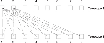
Figure 1. Schematic diagram of the A-MASP GS layout in the two telescopes.
Download figure:
Standard image High-resolution imageAssume that two small telescopes, each having an aperture size of 100 mm, have separations of s = 1.2 m. A linear array of 31 GSs is used and each has an angular gap of θ = 8'' with its neighborhood stars. The first GS and the last GS will have an angular gap of 240''. Therefore, the first and second GS combination will provide a measurement height of Hmax = s/θ = 30 km, which is the maximum measurement height, while the first and last GS combination will provide a measurement height of H = s/((N − 1)θ) = 1000 km, which is the vertical resolution. In such an approach, our A-MASP can measure the seeing profile from the ground to a maximum measurement height of 30 km. Please note that for each GS combination, the two GSs must be located at different telescopes, as shown in Figure 1.
Assume that for the M GSs, the relative image slopes or displacements are either along the longitudinal direction (x component) or perpendicular direction (y components) to the line connecting the centers of the two telescopes. Again, assume that one telescope is located on the original, and the second one is located a distance s from the first one. For any GS combination between two GSs, the field angle of the first GS is assumed to be zero, while the second GS is at an angle of θ relative to the first one and the third one has an angle of 2θ, and so on. The last GS (i.e., number M) has an angle of (M − 1)θ. For N layers of atmospheric turbulence, the first GS measurement slope δx1 is measured with itself over the two telescopes and is the added contribution of each layer located at a height of hn projected along the telescope line of sight
while xn (s) means that the measurement is done in the second telescope, while xn (0) means that the measurement is done in the first telescope. For the first GS, it can be combined with any GS in the other telescope except for the first one. In the case that it is combined with k GS, the measurement slop δx2 is
where θk = (k − 1)θ. Now the covariance between δx1 and δx2 is defined as
where  represents the average over a large number of short-exposure images. The covariance can be eventually calculated as
and similarly, in the y direction we have
where
The coefficient cn is expressed in each layer and is related to the Fried parameter of that layer as

For the circle apertures we used, according to Kellerer (2015), the structure functions I(u, 0) and I(u, π/2) have the forms
where w = 1 + 1.14u−5.5/3 .
The efficient diameter Deff is D + φhn, where φ is the average diameter of the FOV used as a GS, and h is the maximum measurement altitude.
The above equations only apply to one pair of GS combinations. For a linear array of M GSs, there are (M × M − M) combinations that can be used to solve the Fried parameters in each layer. In addition, there are also M combinations that can be used to solve for the overall Fried parameter that includes the turbulence contribution from zero to infinite height. The large number of combinations provides enough redundancy to resolve the seeing Fried parameters, which significantly increases the measurement accuracy (for both the seeing profile and the overall Fried parameter measurements), and is a unique feature for our A-MASP.
3. Simulations
For the performance simulations, we use Monte-Carlo numerical simulations to study the seeing retrieving process. A Kolmogorov phase screen is generated for each atmospheric layer according to Johansson & Gavel (1994). The outer scale L0 is set to be infinity. Two cases are simulated. The first one is for the simulation with a four-layer seeing profile, while the second one is for eight layers. For N layers of turbulence with M GSs, we solve the seeing Fried parameter at each layer using the linear least-squares method by minimizing the sum with the contribution from all (M × M − M) GS combinations
where W(θk) is a weight function, and it is used to weigh each GS combination, i.e., the corresponding height.
For the first simulation, we use four layers of seeing parameters at an average seeing condition measured on the BBSO, in which the associated seeing parameters at the altitudes of 200, 1000, 3000, and 8000 mm were measured with the BBSO 1.6 m NST. The center-to-center separation s between the two telescopes for our A-MASP is 1000 mm, and the diameter for each telescope is 100 mm. According to H = s/θk, the maximum measurement altitude of 8000 m requires θ = 25 8. We use two linear arrays, each with 12 GSs. That is, a linear array of 12 GSs, each with a 258 gap with its neighborhood stars, is uniformly distributed along the x-axis direction. In order to increase the redundancy and thus the retrieved precision, 2 linear arrays, each with 12 GSs and displaced 30'' from each other along the y-axis direction, are used in our simulation. Both 1000 and 2000 images of short-exposure are used to retrieve the results. Table 1 lists the original input seeing parameters and the corresponding retrieved results in each altitude. We can see that if 1000 images are used, the seeing retrieving results have errors of <10%. If we increase the number of images to 2000, the seeing retrieving results have errors <8%.
Table 1. Four-layer Seeing Profile Retrieving Results
| Altitude (mm) | 200 | 1000 | 3000 | 8000 |
|---|---|---|---|---|
| Input (cm) | 12.5 | 22.3 | 42.0 | 70.0 |
| Retrieved (cm): 1000 images | 12.1 | 23.5 | 38.2 | 76.9 |
| Retrieved (cm): 2000 images | 12.0 | 24.0 | 38.9 | 67.9 |
Download table as: ASCIITypeset image
A seeing profile with eight layers can also be retrieved. Now, we use a seeing profile consisting of eight layers located at the altitudes of 0 m (for the ground layer), 1587, 2063, 2500, 3500, 5000, 10,000, and 20,000 m as inputs to retrieve the seeing data at the associated altitudes, as shown in Table 2, in which the low altitude seeing is more interesting and has a high sampling density. The heights of the eight layers are derived in advance by using high-density altitudes to sample the seeing profile, with their normalized peak intensities shown in Figure 2, from which the eight peaks and the associated altitudes can be seen clearly. Again, the center-to-center separation between the two telescopes is still 1000 mm, and the diameter for each telescope is 100 mm. A linear array of 16 GSs, each with a 10'' gap with its neighborhood stars along the x-axis direction, is used. To increase the redundancy and simulation measurement accuracy, two linear arrays, each displaced 20'' in the y-axis direction, are used in this simulation. Table 2 lists retrieved results, while the retrieved results in terms of  are shown in Figure 3. Two-thousand images are used. Compared with the input values, we achieve a Fried parameter error that is less than 7% in each layer.
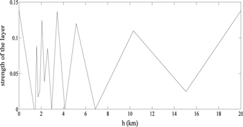
Figure 2. Retrieved strength of turbulence layers (with eight peaks).
Download figure:
Standard image High-resolution image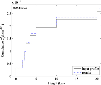
Figure 3. Retrieved  distribution (dash lines), compared with the input values (solid lines).
Download figure:
Standard image High-resolution imageTable 2. Eight-layer Seeing Profile Retrieving Results
| Altitude (mm) | 0 | 1587 | 2063 | 2500 | 3500 | 5000 | 10,000 | 20,000 |
|---|---|---|---|---|---|---|---|---|
| Input (cm) | 10.00 | 10.00 | 10.00 | 10.00 | 10.00 | 10.00 | 10.00 | 10.00 |
| Retrieved (cm): | 9.92 | 10.42 | 9.46 | 9.39 | 9.37 | 9.80 | 10.18 | 9.36 |
Download table as: ASCIITypeset image
4. A-MASP for Real Seeing Profile Measurements
Using numerical simulations, we have demonstrated that the seeing profile can be retrieved precisely. For the simulations, phase screens need to be generated for each layer, and the slope for each GS is calculated as a sum contributed by each layer. This requires intensive computation, especially when the layer number is large. As a result, we only calculate an eight-layer seeing profile. In real seeing measurements, the above process is eliminated, and slopes from each GS can be calculated directly. Therefore, in real measurements the calculation load will be significantly reduced, and a seeing profile with a large layer number can be calculated effectively. Here we present two possible A-MASP configurations that can be deployed for real site measurements, with the detailed specifications listed in Table 3. The first A-MASP is called 1.2 m mode since it has a 1.2 m separation between its two telescopes, while the second is called 0.24 m mode and has a 0.24 m telescope–telescope separation. Except for the telescope–telescope separation, these two A-MASPs are identical, including optics and recorded images for the seeing profile retrieving. Therefore, the same software can be used with the two A-MASPs without any modification (except for the separation s used for the seeing retrieving). For the 1.2 m mode, it can measure the seeing profile up to 30 km, and the Fried parameters in 15 layers are retrieved by using 31 GSs. The 31 GSs are arranged in a linear array, each with an 8'' gap with its neighborhood stars, which results in a vertical resolution of 1000 m. Similarly, for the 0.24 m mode with the same GSs and GS–GS gap, A-MASP can deliver a vertical resolution of 200 mm and a maximum measurement height of 6 km. Therefore, one can use two A-MASPs, one for the seeing profile measurement to a high altitude, and the other for detailed profile measurements around a low altitude.
Table 3. Two possible A-MASP Configurations
| Telescope separation | 1.2 m mode | 0.24 m mode |
|---|---|---|
| Telescope Diameter | 100 mm | 100 mm |
| Guide star separation | 8'' ∼ 240'' | 8'' ∼ 240'' |
| Vertical resolution | 1000 m | 200 m |
| Maximum sample height | 30 km | 6 km |
| Retrieved layers | 15 layers | 15 layers |
Download table as: ASCIITypeset image
For each A-MASP, a camera can be directly attached to the telescope focal plane for image grabbing. Two cameras, each attached to its corresponding telescope, are needed. The two cameras can record images simultaneously by using the camera's image triggers, which are controlled by software. Since each telescope in the A-MASP has an aperture diameter of 100 mm and the seeing profile measurements are conducted at the 0.5 μm wavelength, the telescope can deliver an angular resolution of λ/D = 10 at good seeing conditions. Here D and λ are the telescope diameter and measurement wavelength, respectively. For our A-MASP, the 10 angular resolution will be sampled by at least 2 pixels, which results in an image sampling scale of 05 pixel−1, and this is enough to resolve the solar granules that have a typical size on the order of ∼2''. Solar adaptive optics (Rimmele & Marino 2011) typically uses an 80 mm sub-aperture size with an SHWFS image sampling scale of 10 pixel−1, and have been successfully used for solar granule wavefront sensing. Our A-MASP, with a better image sampling scale (05 pixel−1), should deliver better GS slope measurement. Current solar adaptive optics uses a solar surface region with a size of 8'' × 8'' ∼ 10'' × 10'' as a GS. Since our A-MASP system has a better imaging sampling scale, we will use a solar granule region with a size of 6'' × 6'' as a GS. Figure 4 shows one of the possible GS configurations for our A-MASP, in which each array has 31 GSs with 8'' GS–GS separation in each array, and 2 arrays are used. The small square in the figure represents a GS with a size of 6'' × 6'', and the array to array separation is 40''. To find the GS slope, each GS's displacement is limited to be found in a small local FOV with a size of 15'' × 15'' centering in the ideal position with zero slope. In the case that two linear arrays cannot achieve the required measurement accuracy (i.e., the measurement Fried parameter error must be less than 10%), a more linear array, such as three, can be used to further reduce the measurement errors.

Figure 4. One possible GS configuration for the A-MASP.
Download figure:
Standard image High-resolution image5. Discussions
In Section 4, we discussed two possible A-MASP configurations. In each A-MASP, two small telescopes are assembled together as a rigid unit. For such a system there is a concern that a relative position shift may be induced between the two telescopes during the seeing profile measurements. In our design, a dedicated aluminum alloy frame can be used as the assembly mount that will hold the two small telescopes together. The two small telescopes can be slid into the interfaces on the assembly mount, and the telescope positions as well as the orientations are tightly controlled by mechanical tolerances to ensure that any relative position shifts between the two telescopes are within the allowed tolerance range. Laboratory test using a point image source can be used to measure the relative position shift until such a position shift is in an acceptable range (for example, the induced retrieved r0 error must be less than 5%). The position shift induced by possible flexure distortion of the frame structure can be calculated during the design. Since the physical size of the telescope is small, this is easy to achieve. Finally, in our previous work, we proposed a dedicated algorithm (See Section 5 "Using Two Individual Telescopes" in Ren et al. 2015), which can remove the relative position shift between the two telescopes, and deliver equal performance for retrieving the seeing profile. We can apply these two algorithms to our A-MASP, although the algorithm discussed in this publication is more straightforward and concise.
In order to test the A-MASP seeing profiler with GS using a solar extended structure region, we use 5 × 5 point-source GSs to uniformly sample the 6'' × 6'' small region in the solar surface. As the first step, we calculate the shift values of each guiding star after atmospheric turbulence. Then the shift values of all GSs are averaged to generate the total shifts of the whole region. As the third step, the averaged shifts values can be viewed as the measurement result of a GS with the 6'' × 6'' extended region and are used to retrieve the seeing Fred parameter r0. Two small regions with a separation of 8'' are studied. Only one layer of turbulence is considered, which is located at 1128 m with r0 = 70 mm, which corresponds to a typical isoplanatic angle of 4'' in average seeing conditions on a solar site. The two regions are observed by two 80 mm telescopes with a separation of 1 m. Using Equations (1)–(10) in this publication, r0 can be retrieved. Note that in Equations (1)–(10), the effective diameter is Deff = D + Hφ, where φ is the size of the GS region and has the value of 6'' here, and H is the height of the layer (1128 m). One thousand images are used, and finally the retrieved seeing parameter is r0 = 68.4 mm. In the same condition, we also calculate the seeing parameter using a point-source guiding star as we did in Section 3. Note that in this case, φ = 0 and Deff = D. For the case of a point-source GS, we get the retrieved seeing parameter r0 = 70.6 mm. Comparing the results from point-source and extended GSs, we can see that the difference is about ∼3%, which is acceptable for using point-source GSs to replace extended-region GSs. In our simulation, in an ideal case, a difference of  or
or  in the above two approaches should be equal to 0. However, in a real simulation or measurement, it will not be zero, and thus generates some simulation or measurement errors. Therefore, the difference of this position difference can be used as an indicator to estimate the measurement error for the seeing parameter. We note that the ∼3% seeing parameter error corresponds to a position error of 1.0 × 10⁻³'' on the sky for the
  or
or  .
.
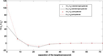
To further study the pupil expansion, we perform a 10-guide-star simulation. The 10 GSs form a linear array. The separation between two neighborhood stars is 8'', so that the first GS forms an angular separation of 0'', 8'', 16''... with itself and another star. Also, the height of the layer is increased to 10,000 m to make the expansion of the pupil more notable. In Figure 5, we plot the simulated and analytical  versus the angular separation between two GSs for both the point-guide-star and extended-region-guide-star methods (the results also apply to
  ). The black dots indicate
  values, which are calculated based on measured images with the extended-region-guide-stars, and black solid line indicate the analytical values (δx1δx2), which are calculated according to Equation (4). When we calculated (δx1δx2), the r0 and height were used as input values, Deff = D + Hφ, and φ = 6''. We can see that the simulated and analytical (δx1δx2) data overlap and fit to each other very well. The red dashed line and the crosses indicate the results of the point-guide-star method. We can see that if the size of the GC region is considered, the variations of the shifts values are reduced because of an averaging effect. Good fittings for both extended-region-guide-stars and point-guide-stars indicate that either one can be effectively used to retrieve the seeing profile accurately. In this simulation, the retrieved value is r0 = 0.0979 m in point-guide-star mode and r0 is 0.1018 m in extended-region-guide-star mode. The two values only have ∼3.8% difference. In fact, since the telescope diameter is replaced with the effective diameter in our calculations and simulations, the Fred parameter r0 can be retrieved by using extended-region GSs.
Figure 5. Simulated and analytical  for the point-guide-star and extended-region-guide-star.
Download figure:
Standard image High-resolution image
Shot noise and low contrast of granule image may also be a concern. The solar wavefront sensing slope is calculated by using cross-correlations between a reference image and a target image in each sub-aperture. Assuming that Nyquist sampling is applied as discussed by Michau et al. (1993), the slope measurement variance for solar correlation can be calculated as
where m = 4 for Nyquist sampling. n is the pixel number of the reference image for the correlation.  is the target image spatial variance (i.e., granulation image contrast variance).
  is the background noise variance. As discussed by Michau et al. (1993) for solar AO wavefront sensing, the typical values are σi = 0.01S, σb = S/500 and 15 × 15 reference sampling pixels (where S is image mean value), which yields a standard deviation of the slope error σ = 1/17 waves on the focal plane of the SHWFS. For our A-MASP, if the small telescope has an aperture diameter of D = 80 mm, an f-number of f/20, and the measurement wavelength is 0.5 μm, the slope error of σ =1/17 waves corresponds to an angle error of 3.8 × 10⁻³'' on the sky. One should note that this calculation is based on typical solar AO wavefront sensing, which works on a fast correction rate of 1000 ∼ 2000 Hz. For the seeing measurement, a low image acquisition speed is acceptable, and thus a better camera can be used to acquire the images.
For the A-MASP, we will use an Andor sCMOS camera (Andor Zyla 4.2 PLUS sCMOS), which has a 30,000 e− well depth and less than 1 e− readout noise at 53 fps with 2048 × 2048 pixels. With this sCMOS camera, it can deliver a background noise σb ≈ S/20,000 (assume only 20,000 e− well depth is used to acquire images). With σi = 0.01S contrast, and 30 × 30 reference sampling pixels, we can achieve a standard deviation of the slope measurement σ = 7.5 × 10⁻⁴ waves, which corresponds to a sky angle of 48 × 10−5. Since we knew that a sky angle error of 10 × 10−3 for the  or
or  corresponds to a seeing parameter measurement error of ∼3%, the retrieved seeing parameter error induced by the position error as a result of the shot noise, granule image contrast and detector noise is much less than 3%, and is not a dominant error for the seeing parameter measurements.
6. Conclusions
We propose A-MASP for precision solar seeing profile measurements. A-MASP consists of two small telescopes, each with a 100 mm aperture. A-MASP uses a linear array of GSs to retrieve the seeing profile. Since A-MASP uses solar granule structures as GSs, in principle, any number of GSs can be used. The retrieved Fried parameter accuracy can be improved by increasing the GS number, i.e., using more linear arrays, which provides an effective approach to improve the seeing profile measurements. We demonstrated that a seeing profile with eight layers with up to 20 km of maximum measurement height can be effectively retrieved with a precision better than 7%. We also show that in real measurements, A-MASP can be designed to measure seeing profiles up to 30 km, with a good vertical resolution. A-MASP is a portable system and can be brought to any potential new site for seeing profile measurement, when no large facility telescope is available. On an existing site where a large telescope is operational, our A-MASP is also useful for solar seeing profile surveys, considering the limited available time with a large telescope as well as the large amount of time required for such measurements. Finally, our A-MASP has the potential to be duplicated in large quantities, and can be used as an accessory device for future solar MCAO systems for routine seeing profile monitoring.
We thank the anonymous referee for valuable comments. This research is supported by a grant from the Mt. Cuba Astronomical Foundation, and also supported by awards from the National Natural Science Foundation of China (NSFC) under grants 11328302 and 11220101001, as well as special funding for Young Researchers of the Nanjing Institute of Astronomical Optics & Technology.