


Abstract
The charge density wave (CDW) in 1T–TiSe2 harbors a nontrivial symmetry configuration. It is important to understand this underlying symmetry both for gaining a handle on the mechanism of CDW formation and for probing the CDW experimentally. Here, based on first-principles computations within the framework of the density functional theory, we unravel the connection between the symmetries of the normal and CDW states and the electronic structure of 1T–TiSe2. Our analysis highlights the key role of irreducible representations of the electronic states and the occurrence of band gaps in the system in driving the CDW. By showing how symmetry-related topology can be obtained directly from the electronic structure, our study provides a practical pathway in search of topological CDW insulators.
Export citation and abstract BibTeX RIS

Original content from this work may be used under the terms of the Creative Commons Attribution 4.0 licence. Any further distribution of this work must maintain attribution to the author(s) and the title of the work, journal citation and DOI.
1. Introduction
Transition metal dichalcogenides have layered crystal structures with the weak van der Waals interaction between the adjacent layers. This feature allows them to be exfoliated in few layers or even monolayers, bringing intensive interest for their appealing electronic and optoelectronic properties [1–6]. Owing to the low dimensionality, many materials undergo a charge density wave (CDW) phase transition [2, 7, 8]. 1T–TiSe2 is a noteworthy examples which shows superconductivity when the CDW is suppressed via doping or pressure [9–14]. The CDW in 1T–TiSe2 is commensurate, forming a 2 × 2 × 2 superlattice [15, 16]. Simultaneous periodic lattice distortion (PLD) [17] was observed from the phonon softening in the  mode [
 is an irreducible representation (IR) at L] [15, 18, 19], indicating the symmetry of the CDW.
The  CDW is nontrivial due to its anisotropic character. It is reminiscent of the d-density wave in strongly correlated systems where the local rotation symmetry is broken [20, 21]. Symmetry is important because it bears on the CDW mechanism [22] and determines whether the CDW nodes in the electronic structure influence superconducting Tc. It also drives directional responses [23] and controls the topology of the system. The key role of symmetry, however, has not been hardly explored in the literature [24–27]. With this motivation, we will elucidate the symmetry properties of the CDW state in 1T–TiSe2 and their connections with the electronic structure and the band topology of the system.
Our analysis starts by considering a system at high temperature, which is described by the bare Hamiltonian  with symmetry group
  . The symmetry elements Ri
of
. The symmetry elements Ri
of  will of course commute with the Hamiltonian, i.e.
 ![$\left[{\hat{R}}_{i},{\hat{H}}_{0}\right]=0$](https://content.cld.iop.org/journals/1367-2630/23/8/083037/revision2/njpac1bf4ieqn7.gif) . When the CDW order develops at low temperatures, the CDW Hamiltonian becomes
. When the CDW order develops at low temperatures, the CDW Hamiltonian becomes  , where
  is to capture the CDW order. As a result, some symmetries
  will be broken when
 ![$\left[{\hat{R}}_{i},{\hat{H}}_{\text{CDW}}\right]=\left[{\hat{R}}_{i},\hat{{\Delta}}\right]\ne 0$](https://content.cld.iop.org/journals/1367-2630/23/8/083037/revision2/njpac1bf4ieqn11.gif) . Most obvious is the breaking of the translation symmetry T since
. Most obvious is the breaking of the translation symmetry T since ![$\left[\hat{T},\hat{{\Delta}}\right]\ne 0$](https://content.cld.iop.org/journals/1367-2630/23/8/083037/revision2/njpac1bf4ieqn12.gif) . [For a commensurate CDW the translation symmetry can be restored by enlarging the unit cell:
. [For a commensurate CDW the translation symmetry can be restored by enlarging the unit cell:  for some integer M such that
 ![$\left[{\hat{T}}_{\text{CDW}},\hat{{\Delta}}\right]=0$](https://content.cld.iop.org/journals/1367-2630/23/8/083037/revision2/njpac1bf4ieqn14.gif) .] So, the symmetry group will be reduced to a subgroup
.] So, the symmetry group will be reduced to a subgroup  of
of  which will contain symmetry elements isomorphic to those that are left invariant under the CDW distortion in
  .
.
The symmetry of the CDW order parameter (OP) will be characterized by the symmetry group of the ordering vectors q. We will assume that the OP is a one-dimensional (1D) IR of the little group  , a subgroup of
  which contains the point-group symmetries that keep q invariant. By 1D IR we mean that the OP is an eigenstate of point group symmetry
  with eigenvalue either +1 or −1, i.e.
  . Note that the broken symmetries in the CDW state also include those associated with eigenvalues of −1, which are related to the ordering vectors for the direction of the atomic displacements [28].
2. Symmetry of 1T–TiSe2
Pristine 1T–TiSe2 crystallizes in a hexagonal lattice structure with point group D3d and space group  . Its low-temperature phase is the triple-q CDW state with ordering vectors
  ,
,  , and
, and  , which connect Γ and the three inequivalent L points (L1,2,3), see figure 1(a). The little group of L2 contains point-group elements {
![$E,{2}_{[100]},{m}_{[100]},\overline{1}$](https://content.cld.iop.org/journals/1367-2630/23/8/083037/revision2/njpac1bf4ieqn26.gif) } as the group C2h
, which has four 1D IRs Ag
, Bg
, Au
, and Bu
(table 1). With 3[001] we obtain conjugate representations for L2 and L3. Including translation T of the Bravais lattice, IRs of the OP can be written as
} as the group C2h
, which has four 1D IRs Ag
, Bg
, Au
, and Bu
(table 1). With 3[001] we obtain conjugate representations for L2 and L3. Including translation T of the Bravais lattice, IRs of the OP can be written as

We describe the OP for a given IR by the vector  where the
  accompanying the IR determines the symmetry group (isotropy group). The energy is better for the maximal isotropy group [29, 30] so we will take
  .
.
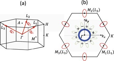
Figure 1. (a) Bulk BZ and the CDW ordering vectors Q1,2,3 of 1T–TiSe2. (b) Schematic FS of the pristine 1T–TiSe2 in the kz = 0 plane. Three hole-pockets at Γ are marked by the thick blue circle. Electron pockets at the L points are shown by red ellipses. The green dotted lines around Γ show an i-wave CDW gap function, which supports 12 line nodes on the FS of the CDW state.
Download figure:
Standard image High-resolution imageTable 1. Character table for the point-group symmetry C2h
at the point L. The CDW OP will be one of the IRs  . To avoid confusion, the conduction band at L is labeled with the IR given in parentheses in column 1.
| C2h | E | C2 | σh | i |
|---|---|---|---|---|
 (Ag
) (Ag
) | 1 | 1 | 1 | 1 |
 (Bg
) (Bg
) | 1 | −1 | −1 | 1 |
 (Au
) (Au
) | 1 | 1 | −1 | −1 |
 (Bu
) (Bu
) | 1 | −1 | 1 | −1 |
Referring to the symmetries of OPs in table 1, we can read off the space groups for the four CDW states. The states with mirror eigenvalue −1 do not have a mirror plane but only the glide plane {m[100]|001}, where the accompanying  translation produces a complementary −1. Similarly states with the parity eigenvalue −1 respect the combined symmetry
  (
( ). As
). As  , there is inversion symmetry with respect the center at
  . We thus conclude that the space group for
  and
and  is
is  (no. 164) and for
  and
and  is
is  (no. 165).
3. Hamiltonian
The normal state band structure of TiSe2 using the generalized gradient approximation (GGA) without spin–orbit coupling (SOC) is shown in figure 2(a). There are three bands crossing the Fermi level at Γ and one band crossing at L. The states at Γ consist of the two-fold Eg and one-fold A2u representations whereas the state at L belongs to the Ag representation. The mean field k ⋅ p Hamiltonian for the CDW can be expressed as

where the basis  is taken and

The prime on the summation in equation (2) indicates that only low-energy or k states in the folded Brillouin zone (BZ) are considered (spin index is omitted for brevity). The states at the Γ and L's points as well as at the A and M points are coupled by the CDW gaps. Also, because q vectors connect the Γ and A points, these four points can be written together. The states at Γ and L's can be described by  :
:

where  and
and  account for the normal-state band structure around Γ and L's, respectively. In
  , the former two operators stand for the Eg
states and the last one is for A2u
. In
, the former two operators stand for the Eg
states and the last one is for A2u
. In  , the three bands at the three L's are included with k being relative to the corresponding L's. The CDW gap ΔΓL
is a 3 × 3 matrix, where the matrix element Δij
refers to the CDW potential between
, the three bands at the three L's are included with k being relative to the corresponding L's. The CDW gap ΔΓL
is a 3 × 3 matrix, where the matrix element Δij
refers to the CDW potential between  and
and  . We will mainly discuss
  and
and  . The off-diagonal element
  , which is induced by the second secondary OP, is expected to be weak.
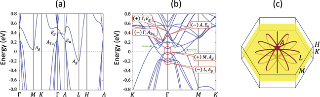
Figure 2. Band structures without SOC for (a) the normal state and (b) the  CDW state. Energies are given relative to the Fermi energy. In (a), the IRs for relevant states at the symmetry points are listed. In (b), the parity eigenvalues of states at Γ are given in parentheses along with the original k points and IRs. Green arrows point to the CDW nodes. (c) Illustration of the 12 nodal lines piercing through the kz
= 0 plane (in yellow) in the folded BZ. The nodal lines were determined from the zeros of the CDW gap function on the FS based on Δ32(k) in equation (14).
CDW state. Energies are given relative to the Fermi energy. In (a), the IRs for relevant states at the symmetry points are listed. In (b), the parity eigenvalues of states at Γ are given in parentheses along with the original k points and IRs. Green arrows point to the CDW nodes. (c) Illustration of the 12 nodal lines piercing through the kz
= 0 plane (in yellow) in the folded BZ. The nodal lines were determined from the zeros of the CDW gap function on the FS based on Δ32(k) in equation (14).
Download figure:
Standard image High-resolution imageThe Hamiltonians can be determined using the symmetry constraints as follows:


where  , −k, and
  are momenta under 3[001],
  , and m[100], respectively. We define the [100] direction to be x and [001] to be z. The relevant symmetry operators are

with

and

where  and
and  is the eigenvalue of the OP for operation
  . Note that the eigenvalue in front of
  takes
takes  because Γ is connected to A via the sum of three ordering vectors Qi
. But, the eigenvalue at
because Γ is connected to A via the sum of three ordering vectors Qi
. But, the eigenvalue at  takes
takes  because a sum of two Qi
connects Γ and M. As
because a sum of two Qi
connects Γ and M. As  is block-diagonal, equations (5)–(7) determine the form of
  ,
,  , and ΔΓL
, see appendix
, and ΔΓL
, see appendix  reflects the symmetries of the OP via the CDW gap matrix as follows


where  ,
,  (=±1) and
  . The four IRs
  are obtained by taking
  , and (−1, 1), respectively (listed also in table 1).
Although the  CDW OP has an f-wave symmetry [31], the CDW gap functions may be of different symmetry depending on IRs of the composite bands as we will show below. It can be shown that the gap functions for the
  CDW state to the lowest order of k are:

where λ, λ''s are taken to be real. The other terms can be obtained using the rotation symmetry, see appendix
Figure 2(b) presents the band structure of the CDW state in the presence of PLD. We can see that the CDW gap size (∼0.1 eV) is not small and the band structure is complex as a result of many band foldings. Now there are two CDW nodes (band crossings between the conduction and valence bands), one on the  line and the other along the
  line. Taking into account the rotation and time-reversal symmetries, there are 12 nodes on the kz
= 0 plane. A full BZ exploration of the band structure shows that these nodes persist away from the kz
= 0 plane and yield nodal lines in the BZ, see figure 2(c). Band structures for different kz
values are given in appendix
line. Taking into account the rotation and time-reversal symmetries, there are 12 nodes on the kz
= 0 plane. A full BZ exploration of the band structure shows that these nodes persist away from the kz
= 0 plane and yield nodal lines in the BZ, see figure 2(c). Band structures for different kz
values are given in appendix
4. Ginzburg–Landau theory
We turn now to discuss the Ginzburg–Landau theory for the  CDW state. Images of the primary OP (
 mode)
mode)  under various symmetry operations are:

so that the free-energy density which satisfies symmetries of the pristine state to the fourth order becomes:

Here α < 0 when T < Tc for nonzero  and β > 0 for stability. Therefore, we seek a secondary OP that is linearly coupled to the primary OP
  , i.e. we look for coincidence of the primary and secondary OPs (appendix
  will also have three components with the coupling energy

where  follows the rules in equation (B2) except that m[100],
  , and
, and  are without the minus signs. The symmetry conditions dictate that the components of the secondary OP take ordering vectors
  ,
,  , and
, and  and that they belong to IR
  . In addition to the terms similar to equation (B5), the free energy for the secondary OP can contain the cubic term ζ1
ζ2
ζ3. Besides, coexistence of
. In addition to the terms similar to equation (B5), the free energy for the secondary OP can contain the cubic term ζ1
ζ2
ζ3. Besides, coexistence of  and
and  OPs will induce a third (second secondary) OP φ in higher order as

where φ, which we call IR  , is parity-odd, mirror-odd and belongs to the ordering vector
  . Close to Tc, ζ is proportional to ϕ square and thus ψ is proportional to ϕ cube, so that the symmetry characters of
  (
( ) are the same as
  and those of
  are identical to
  . Incidentally, the coincident
  OP will also be present in the other three CDW states, accompanied by the corresponding third OPs.
5. IRs of bands
Although the gap functions in equation (14) all vanish at k = 0, the folded bands still result in threefold degeneracy. But, this threefold degeneracy should not occur as it is not robust in the D3d group. This can be understood, however, because the concurrent  mode produces couplings among the bands at L points (also among the M points): the triplet from L's then splits into a singlet A1u
state and a doublet Eu
state without breaking symmetry [32]. We emphasize that the parity of the folded bands changes from even to odd due to the CDW OP. In general, the IR of a folded band is the product of IRs of the unfolded band and the OP, written as:
mode produces couplings among the bands at L points (also among the M points): the triplet from L's then splits into a singlet A1u
state and a doublet Eu
state without breaking symmetry [32]. We emphasize that the parity of the folded bands changes from even to odd due to the CDW OP. In general, the IR of a folded band is the product of IRs of the unfolded band and the OP, written as:

This is our key finding, which is especially useful for investigating topology. By contrast, folded bands from M's to Γ, through the secondary  OP, split into an Ag
and two Eg
states. As for the bands from A, their parities change sign because of the
OP, split into an Ag
and two Eg
states. As for the bands from A, their parities change sign because of the  mode. These arguments are well corroborated by our independent first-principles band structure results, see figure 2(b).
Note that the gap function of two composite bands has the symmetry of the direct product of the IRs of the two bands. For instance, if the closest conduction band is IR A1u and the valence band is IR A2u , the associated gap function will be IR A2g (=A1u ⊗ A2u ) that is also known as the i wave outlining a sin(6ϕ) profile, figure 1(b).
6. Topology
We recall at the outset [33] that in the presence of inversion and time-reversal symmetries, SOC-free systems can be classified into semimetals with even or odd number of bulk line nodes, which can be labeled with a set of  invariants obtained from the product of parity eigenvalues of filled bands at the four parity-invariant momenta in a BZ plane. The line nodes are gapped by the SOC to yield weak topological insulators [34, 35].
In the CDW state, the parity-product at M, L, and A points in the folded BZ will be trivial, so that only the Γ point remains relevant. The reason is that the original and folded bands hybridize into symmetric and antisymmetric combinations resulting in a parity-product of −1, and even number of such pairs will yield a net product of +1. In the case of no band inversion, the parity-product at Γ of the CDW state is related to the strong topological invariant of the pristine state. Therefore, the strong topological invariant of the CDW state will be determined by the number (mod 2) of band inversions which involve parity switching beyond the topology of the normal state.
Our DFT calculations show that the pristine and the  CDW states are both topologically trivial. Figure 2(b) shows that the three bands at Γ (Eu
and A2u
bands) hybridize with three pristine bands at L points without changing parity yielding a net parity-product of +1. Also, the two bands at A (Eu
symmetry) hybridize with two of three bands at the M points and maintain the parity-product of +1. An even number of nodal rings is thus expected to pierce through the kz
= 0 plane as is seen to be the case in figure 2(c). In this connection, we have further analyzed the band structure of the
CDW states are both topologically trivial. Figure 2(b) shows that the three bands at Γ (Eu
and A2u
bands) hybridize with three pristine bands at L points without changing parity yielding a net parity-product of +1. Also, the two bands at A (Eu
symmetry) hybridize with two of three bands at the M points and maintain the parity-product of +1. An even number of nodal rings is thus expected to pierce through the kz
= 0 plane as is seen to be the case in figure 2(c). In this connection, we have further analyzed the band structure of the  CDW state (not shown for brevity) to show that it is a topologically nontrivial semimetal consistent with equation (19).
7. Conclusion and discussion
We have presented an in-depth analysis of the symmetries as well as the topology of the electronic structure of bulk 1T–TiSe2 CDW. Our first-principles calculations show that the CDW state hosts a nodal band structure in which the nodes are protected by symmetry and topology resembling that of the Dirac nodes in the spin-density-wave phase of iron pnictides [36, 37]. The existing topological theory in this connection only considers spin-density-wave states [38, 39] in terms of  classification of three-dimensional insulators, but questions of symmetry properties of the density waves and their connection to the normal states have not been addressed. We resolve these questions by successfully connecting the symmetry and topology of the electronic IRs of the normal and CDW phases.
We emphasize that in our theory when both the time-reversal and inversion symmetries are preserved, inclusion of the SOC gaps band crossings for out-of-plane n-fold (n > 2) rotation axis to protect the Dirac nodes, but it does not change the parity of the bands. Although the CDW OP might change the IR and parity of the folded band, it does not always produce band inversion. We discuss the application of our theory to the band structure based on the GGA density functional, which yields a semimetallic normal state with an energy overlap (indirect negative band gap) between the conduction and valence bands. On the experimental side, there has been a longstanding debate whether the normal state of 1T–TiSe2 is a semimetal [40–42] or a semiconductor [32, 43]. Our study however is not concerned with such details of the band structure. Our results are intended to be generic in nature and are not sensitive to the density functional used. The question of sensitivity of the band structure of 1T–TiSe2 to exchange–correlation functional, Hubbard U, and van der Waals interactions has been explored extensively in the literature [44–46]. Correlations are generally found to reduce the band overlap in better accord with experimental results. This is also the case in our first-principles band structure of 1T–TiSe2 obtained with the modified Becke–Johnson (mBJ) meta-GGA density functional, which correctly captures the bandgap correction and reproduces an insulating electronic state, see appendix
Figure 3 shows the pressure effect on the electronic structure of bulk 1T–TiSe2. The energy overlap is seen to be retained under moderate pressures as is the CDW order. This suggests that a topological phase transition in the CDW state can be achieved by applying hydrostatic pressure. By showing how symmetry-related topology can be obtained directly from the electronic structure, our study provides a guide in search of topological CDW phases. Our analysis can be generalized straightforwardly to consider other spontaneous symmetry-breaking phases.
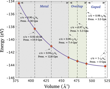
Figure 3. Energy as a function of volume (hydrostatic pressure) of 2 × 2 × 2 bulk 1T–TiSe2 obtained using the mBJ meta-GGA density functional without SOC. The change in lattice parameters and associated hydrostatic pressure are marked. Color regions identify the CDW gapped (white), CDW semimetal (green), and normal metal (gray) states. The system evolves from a large gap CDW insulator to a CDW semimetal for c/a = 0.97c0/a0) and a non-CDW metallic state for c/a = 0.96c0/a0. a0 and c0 (a and c) define the lattice constants at zero (finite) pressure.
Download figure:
Standard image High-resolution imageAcknowledgments
SMH is supported by the Ministry of Science and Technology (MoST) in Taiwan under Grant No. 105-2112-M-110-014-MY3 and also by the NCTS of Taiwan. He also acknowledges support from Academia Sinica's Short-term Visiting Program for Domestic Scholars. The work at TIFR Mumbai is supported by the Department of Atomic Energy of the Government of India under Project No. 12-R&D-TFR-5.10-0100. The work at Northeastern University was supported by the US Department of Energy (DOE), Office of Science, Basic Energy Sciences Grant No. DE-SC0019275 (materials discovery for QIS applications) and benefited from Northeastern University's Advanced Scientific Computation Center and the National Energy Research Scientific Computing Center through DOE Grant No. DE-AC02-05CH11231.
Data availability statement
The data that support the findings of this study are available upon reasonable request from the authors.
Appendix A.: Hamiltonian without SOC
Here we discuss the construction of our mean-field 2 × 2 × 2 CDW Hamiltonian without SOC for bulk 1T–TiSe2. It is written as

where the prime indicates that k runs over states near the Fermi surfaces (FS) and

in the basis  . Based on our first-principles calculations, the normal-state band structure near the Fermi level consists of three valence states at the Γ point, two valence states at the A point, and a conduction band whose minimum locates at each L point. The L-point conduction band adiabatically evolves into bands at the M point, see figure 2(a) of the main text. The two valence bands at Γ are comprised of Eg
IR whereas the third band belongs to A2u
(table 2). The bands at A have the IR Eu
whereas at the L and M, they have Ag
IR (table 1). For
. Based on our first-principles calculations, the normal-state band structure near the Fermi level consists of three valence states at the Γ point, two valence states at the A point, and a conduction band whose minimum locates at each L point. The L-point conduction band adiabatically evolves into bands at the M point, see figure 2(a) of the main text. The two valence bands at Γ are comprised of Eg
IR whereas the third band belongs to A2u
(table 2). The bands at A have the IR Eu
whereas at the L and M, they have Ag
IR (table 1). For  , which contains three creation operators for the hole pockets around Γ,
  , we assign Eg
to the first two operators and A2u
to the last operator. For
, we assign Eg
to the first two operators and A2u
to the last operator. For  , we denote
  . As for ψL
k
, it contains three creation operators for the electron pockets around the three L points,
. As for ψL
k
, it contains three creation operators for the electron pockets around the three L points,  . Replacing L by M, we obtain
  .
.
Table 2. Character table for the point group D3d. Only Eg and A2u IRs for the three valence bands are shown.
| D3d | E | 2C3 | 3C2 | i | 2S6 | σh |
|---|---|---|---|---|---|---|
| Eg | 2 | −1 | 0 | 2 | −1 | 0 |
| A2u | 1 | 1 | −1 | −1 | −1 | 1 |
We will mainly consider the CDW potentials among the bands at Γ and L points. Other potentials can be constructed along similar lines. We first examine

where  and
and  account for the normal-state band structure around Γ and L's, respectively. In these expression,
  ,
,  and ΔΓL
are all 3 × 3 matrices written as
and ΔΓL
are all 3 × 3 matrices written as


Δij (k) will be regarded as the CDW potential between Γi and Lj . The Hamiltonians can then be written down according to the symmetry constraints as:


where  , −k, and
  are momenta under (counterclockwise) 3[001],
  , and m[100], respectively. We define the [100] direction to be x and [001] to be z. The relevant symmetry operators would be k-dependent and are block-diagonal as
We choose


Note that here we adopt a representation in which  ,
,  ,
,  and
and  matrices are diagonal, where the diagonal elements are the eigenvalues of the corresponding symmetries at various symmetry points. In this basis, the
  and
and  matrices are non-diagonal for the Eg
and Eu
states. As for the L and M points, they involve large momentum transfers. For instance, we set
matrices are non-diagonal for the Eg
and Eu
states. As for the L and M points, they involve large momentum transfers. For instance, we set  under 3[001]; while under m[100], which leaves L2 invariant and interchanges L1 and L3,
  and
and  .
.
A.1. Bare Hamiltonians
A.1.1. Hamiltonian at Γ
We will write down the Hamiltonian at  . Here it is easier to use a basis that makes the three-fold rotation operator diagonal. The basis is unitarily transformed as
  and the symmetry operators transform, for instance, as
  , where the unitary matrix

In this 'tilde' basis, the symmetry operators are

where the last operator is the time-reversal operator with complex conjugation K. This tilde Hamiltonian follows the symmetry constraints


By taking  and defining k± = kx
± iky
, symmetry conditions require that for
and defining k± = kx
± iky
, symmetry conditions require that for 

for 

for 

and for 

respectively. The Hamiltonian up to second order is:

Here  and all parameters a, a', b, b', c, c', d, ɛ1, and ɛ2 are real. Finally, we transform
  back to
  by
by

A.1.2. Hamiltonians at L and M
The Hamiltonian at L's  is identical to
  , and can be written as

Here we assume that within the low-energy region, the three bands are independent. The symmetry operators are then given by

Similar as before, we conclude that


A.1.3. Hamiltonians at A
Although the conduction band (Ag ) extends monotonically along L–M, in some calculations the band structure shows a band inversion along Γ–A, where the Eg valence bands switch with the Eu conduction bands. We consider this case in which the valence band becomes IR Eu at A.
The Eu
bands are two-fold degenerate at A, where they are described by the same Hamiltonian (with different parameters) as the upper 2 × 2 block of  in equation (A25). In addition, we show the coupling Hamiltonian between the Eg
and the Eu
bands in
in equation (A25). In addition, we show the coupling Hamiltonian between the Eg
and the Eu
bands in  . In the basis where the symmetry operators for the Eu
bands take the form
. In the basis where the symmetry operators for the Eu
bands take the form

the k ⋅ p model will read

with real parameters t1 and t2. The coupling Hamiltonian indicates anticrossing among the Eg and Eu bands.
A.2. CDW gap functions
The gap functions in equations (5)–(7) follow


where  are eigenvalues of the corresponding operations for the OP. The allowed values for ηI
and ηM
are ±1. The four IRs
are eigenvalues of the corresponding operations for the OP. The allowed values for ηI
and ηM
are ±1. The four IRs  have symmetries with (ηI
, ηM
) = (1, 1), (1, −1), (−1, −1), (−1, 1), respectively. To obtain the gap functions, we have, through equations (A33) and (A34),
have symmetries with (ηI
, ηM
) = (1, 1), (1, −1), (−1, −1), (−1, 1), respectively. To obtain the gap functions, we have, through equations (A33) and (A34),
In particular, the gap functions associated with L2, which is invariant under both inversion and the mirror symmetry, are:


So the gap functions for the four CDW states to lowest order in k are:


Two functions in the brackets are assumed to combine linearly. The remaining gap functions can be obtained via the three-fold rotations as follows. From equation (A32),
Therefore,

For the CDW gap functions among the Eu valence bands at A and the conduction bands at M's, an analysis along the preceding lines yields:


where the momentum k is relative to the A point and the subscript 4, 5 are used to denote the two Eu bands.
Appendix B.: Ginzburg–Landau theory for the two OPs
We examine the Ginzburg–Landau theory for primary and secondary OPs. The primary OP  is taken to belong to the
  IR (IR), which is delineated by

where Au
is an IR in the point group C2h
(little co-group at L) and  stand for translational representations. The 3D ordering vectors are defined by
  ,
,  , and
, and  . The images of
  under symmetry operations in the space group are

Translations by a1,2,3 will produce minus signs due to the oscillating nature of the CDW. From the collection of these images, one realizes that by treating  as an ordinary coordinate vector
  , the transformations correspond to those in the point group Th
. In other words, this is a homomorphism: the space group generates in the vector space of
, the transformations correspond to those in the point group Th
. In other words, this is a homomorphism: the space group generates in the vector space of  the point group Th
. For other three IRs (
the point group Th
. For other three IRs ( ), it is straightforward to obtain the associated images, which are similar to those of
  with modifications at m[100] and
  . Their image groups are also Th
.
. Their image groups are also Th
.
The secondary OP  also transforms as the
  IR:
IR:

The secondary OP has the Ag
symmetry and importantly it describes a 2D CDW with ordering vectors  ,
,  , and
, and  . The images of
  under the symmetry operations are

Note that a translation in a3 has no effect due to the 2D character. Now the space group generates the point group T for  . Incidentally, the image group for
  IR is group T and is Th
for both
IR is group T and is Th
for both  and
and  IRs.
IRs.
The Ginzburg–Landau free energy for the primary OP  is invariant for the group Th
and it can be written as:
is invariant for the group Th
and it can be written as:

where  is defined. It is known that to have a conclusive phase diagram, sixth-degree terms,

are required [29, 30]. When T < Tc and α < 0, a CDW state for nonzero  becomes the ground state. Moreover, only the so-called first type of CDW phases are possible [29, 30]: either of
  ,
,  , or
, or  . The free energies for these three phases are given by

where M = I, II, III, and


An analysis of the first-order transitions between these phases is outside of scope of this paper. We will assume that the M = I phase is the favorable one for given parameters.
The free energy for the secondary OP is

The expansion of the free energy to the fourth degree is sufficient for our discussion. Because the vector space of  has group T symmetry, a cubic term is observed, and the lowest-degree coupling form reads as

in which the primary OP is quadratic and the secondary OP is linear.
The coupling with linear ζ indicates that the secondary OP will coincide with the primary OP. To see this, we reduce the problem by taking ϕ = ϕ1 = ϕ2 = ϕ3 and ζ = ζ1 = ζ2 = ζ3, omit the sixth degree terms and obtain the total free energy as

The optimal values of ϕ and ζ ( and
and  ) are obtained from
  that give


Based on the fact that the secondary OP is induced by the primary OP, we demand that  when
when  , suggesting that α' > 0 as well as γ'2 − 4α'β' < 0.
For nonzero  , it happens when
  , which indicates that Tc is modified by the nonzero of the secondary OP. Replacing
  in equation (B15) by equation (B14) yields the cubic equation,

If the constant term λα/β is finite, the cubic equation always has a real root, explaining the coincidence of the primary and secondary OPs. Close to Tc when OPs are small,  and thus
  .
.
Appendix C.: Computational details
The first-principles calculations were performed with the projector augmented wave method within the DFT [47] framework as implemented in the VASP code [48, 49]. The GGA with the Perdew–Burke–Ernzerhof parameterization and mBJ meta-GGA were used to include the exchange–correlation effects [50, 51]. We used a plane wave energy cut-off of 380 eV and a Γ-centered 12 × 12 × 8 k-mesh to sample the bulk BZ of 1T–TiSe2. To access the nodal lines in the full BZ, we constructed a tight-binding model Hamiltonian by projecting first-principles results onto Wannier orbitals using the VASP2WANNIER90 interface [49, 52]. The Ti d and Se p states were included in the construction of Wannier functions.
Appendix D.: Band structure of the L1− CDW state and nodal lines
We present the ab initio band structure of the CDW state on various kz
planes in figures 4(a)–(f). The band structure in figure 4(a) shows the states at the kz
= 0 plane, which is the same band structure that is presented in the main text. The bands are seen to cross at discrete points along the Γ–K and Γ–M directions at an energy ∼+0.1 eV above the Fermi level. With an increase in the kz
values, the band crossings start lowering their energies and finally merge into the Γ-point on the  plane at an energy ∼−0.05 eV, see figure 4(e). On further increasing the kz
value to
plane at an energy ∼−0.05 eV, see figure 4(e). On further increasing the kz
value to  , the bands become gapped with a clear band gap in the band structure. A full BZ exploration of the band structure shows that the nodal points trace out the continuous lines which pass through the kz
= 0 plane as shown in figure 4(g). We find a total of 12 nodal lines which cross along the Γ–A direction in the BZ. These results are in accord with the theoretical analysis presented above and in the main text.
, the bands become gapped with a clear band gap in the band structure. A full BZ exploration of the band structure shows that the nodal points trace out the continuous lines which pass through the kz
= 0 plane as shown in figure 4(g). We find a total of 12 nodal lines which cross along the Γ–A direction in the BZ. These results are in accord with the theoretical analysis presented above and in the main text.

Figure 4. Bulk structure of the  CDW state with PLD at the selected kz
planes. (a) kz
= 0, (b)
CDW state with PLD at the selected kz
planes. (a) kz
= 0, (b)  , (c)
, (c)  , (d)
, (d)  , (e)
, (e)  , and (f)
  . The bulk nodal band crossings are absent at the
  plane. (g) Calculated nodal-lines crossings in the BZ. Light red plane marks the kz
= 0 plane. The color scale highlights the nodal band crossing energy relative to the Fermi energy.
plane. (g) Calculated nodal-lines crossings in the BZ. Light red plane marks the kz
= 0 plane. The color scale highlights the nodal band crossing energy relative to the Fermi energy.
Download figure:
Standard image High-resolution imageAppendix E.: Band structures under pressure
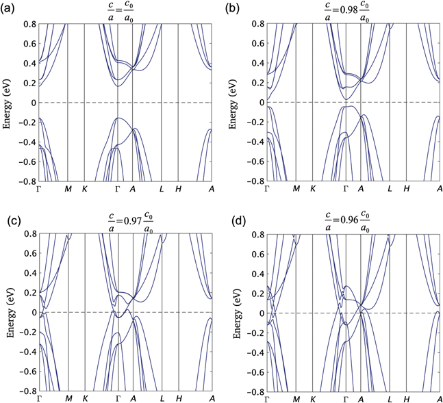
Figure 5 shows the band structure of 1T–TiSe2 2 × 2 × 2 superlattice obtained with mBJ meta-GGA for various hydrostatic pressures. The band structure for c/a = c0/a0 [c and a (c0 and a0) are the lattice constants of pressurized (pristine) 2 × 2 × 2 1T–TiSe2] is insulating with a well-defined gap between the valence and conduction bands. Due to this bandgap, the A2u band at Γ does not show a band inversion. As we decrease c/a to apply a hydrostatic pressure, the bandgap decreases and finally vanishes for c/a = 0.97c0/a0, realizing a metallic state. There is a band inversion between valence and conduction bands, realizing multiple nodal crossings for c/a = 0.96c0/a0. With further lowering of the lattice parameters, the overlap between the valence and conduction bands increases without showing any band hybridizations. This implies that the system is metallic without any CDW order at high pressures.
Figure 5. The bulk band structure of a 2 × 2 × 2 superlattice of 1T–TiSe2 under hydrostatic pressure. (a) c/a = c0/a0, (b) c/a = 0.98c0/a0, (c) c/a = 0.97c0/a0, and (d) c/a = 0.96c0/a0. A CDW insulator to a normal metal transition is seen to take place with pressure.
Download figure:
Standard image High-resolution image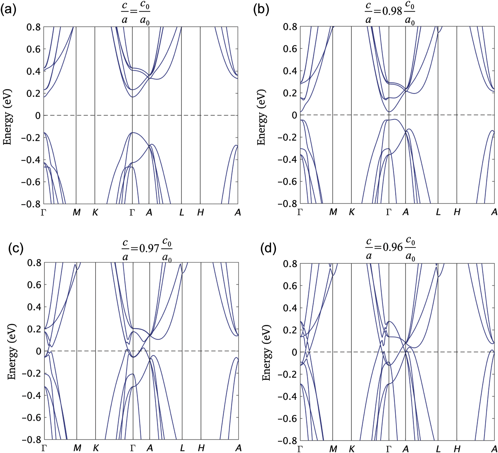